| Issue |
A&A
Volume 576, April 2015
|
|
|---|---|---|
| Article Number | A127 | |
| Number of page(s) | 14 | |
| Section | Extragalactic astronomy | |
| DOI | https://doi.org/10.1051/0004-6361/201424996 | |
| Published online | 17 April 2015 | |
Physical properties of z > 4 submillimeter galaxies in the COSMOS field
1
Department of Physics, University of Zagreb,
Bijenička cesta 32,
10000
Zagreb,
Croatia
e-mail:
This email address is being protected from spambots. You need JavaScript enabled to view it.
2
Argelander Institute for Astronomy, Auf dem Hügel 71, 53121
Bonn,
Germany
3
Department of Astronomy, Cornell University,
220 Space Sciences Building,
Ithaca, NY
14853,
USA
4
Max Planck Institut für Astronomie, Königstuhl 17, 69117
Heidelberg,
Germany
5
Department of Astronomy, California Institute of
Technology, MC 249-17, 1200 East
California Blvd, Pasadena, CA
91125,
USA
6
Spitzer Science Center, 314-6 Caltech,
Pasadena, CA
91125,
USA
7
INAF–Istituto di Radioastronomia, via Gobetti 101,
40129
Bologna,
Italy
8
INAF–Osservatorio Astronomico di Bologna, via Ranzani
1, 40127
Bologna,
Italy
9
Núcleo de Astronomía, Facultad de Ingeniería, Universidad Diego
Portales, Av. Ejército
441, Santiago,
Chile
10
CSIRO Australia Telescope National Facility, PO Box 76,
Epping, 1710
NSW,
Australia
11
Research School of Astronomy and Astrophysics, Australian National
University, Weston
Creek, 2611
ACT,
Australia
12
National Radio Astronomy Observatory, PO Box 0, Socorro, NM
87801,
USA
13
Yale Center for Astronomy and Astrophysics, Physics Department,
Yale University, PO Box
208120, New Haven,
CT
06520-8120,
USA
14
Harvard-Smithsonian Center for Astrophysics, 60 Garden
Street, Cambridge,
MA
02138,
USA
15
Aix Marseille Université, CNRS, LAM (Laboratoire d’Astrophysique
de Marseille) UMR 7326, 13388
Marseille,
France
16
Department of Physics, University of Helsinki,
PO Box 64, 00014
Helsinki,
Finland
17
Max-Planck-Institut für Radioastronomie,
Auf dem Hügel 69, 53121
Bonn,
Germany
18
Space Telescope Science Institute, 3700 San Martin Drive, Baltimore, MD
21218,
USA
19
Sorbonne Universités, UPMC Univ Paris 06, UMR 7095, Institut
d’Astrophysique de Paris, 75005
Paris,
France
20
Institut d’Astrophysique de Paris, UMR 7095 CNRS, Université
Pierre et Marie Curie, 98bis
boulevard Arago, 75014
Paris,
France
21
Department of Physics and Astronomy, University of
California, Riverside, CA
92521,
USA
22
Max-Planck-Institut für Extraterrestrische Physik,
Postfach 1312, 85741
Garching bei München,
Germany
23
Astronomy Centre, Department of Physics and Astronomy, University
of Sussex, Falmer,
Brighton
BN1 9QH,
UK
24
National Radio Astronomy Observatory, 520 Edgemont Road, Charlottesville, VA
22903,
USA
25
Dark Cosmology Centre, Niels Bohr Institute, University of
Copenhagen, Juliane Mariesvej
30, 2100
Copenhagen,
Denmark
Received: 16 September 2014
Accepted: 3 December 2014
Abstract
We investigate the physical properties of a sample of six submillimeter galaxies (SMGs) in the COSMOS field, spectroscopically confirmed to lie at redshifts z> 4. While the redshifts for four of these SMGs were previously known, we present here two newly discovered zspec> 4 SMGs. For our analysis we employ the rich (X-ray to radio) COSMOS multi-wavelength datasets. In particular, we use new data from the Giant Meterwave Radio Telescope (GMRT) 325 MHz and 3 GHz Jansky Very Large Array (VLA) to probe the rest-frame 1.4 GHz emission at z = 4, and to estimate the sizes of the star formation regions of these sources, respectively. We find that only oneSMG is clearly resolved at a resolution of 0''̣6 × 0''̣7 at 3 GHz, two may be marginally resolved, while the remaining three SMGs are unresolved at this resolution. Combining this with sizes from high-resolution (sub-)mm observations available in the literature for AzTEC 1 and AzTEC 3 we infer a median radio-emitting size for our z> 4 SMGs of (0''̣63 ± 0''̣12) × (0''̣35 ± 0''̣05) or 4.1 × 2.3 kpc2 (major × minor axis; assuming z = 4.5) or lower if we take the two marginally resolved SMGs as unresolved. This is consistent with the sizes of star formation regions in lower-redshift SMGs, and local normal galaxies, yet higher than the sizes of star formation regions of local ultraluminous infrared galaxies (ULIRGs). Our SMG sample consists of a fair mix of compact and more clumpy systems with multiple, perhaps merging, components. With an average formation time of ~280 Myr, as derived through modeling of the UV IR spectral energy distributions, the studied SMGs are young systems. The average stellar mass, dust temperature, and IR luminosity we derive are M⋆ ~ 1.4 × 10¹¹ M⊙, Tdust ~ 43 K, and LIR ~ 1.3 × 10¹³L⊙, respectively. The average LIR is up to an order of magnitude higher than for SMGs at lower redshifts. Our SMGs follow the correlation between dust temperature and IR luminosity as derived for Herschel-selected 0.1 <z< 2 galaxies. We study the IR-radio correlation for our sources and find a deviation from that derived for z< 3 ULIRGs (⟨ qIR ⟩ = 1.95 ± 0.26 for our sample, compared to q ≈ 2.6 for IR luminous galaxies at z< 2). In summary, we find that the physical properties derived for our z> 4 SMGs put them at the high end of the LIR–Tdust distribution of SMGs, and that our SMGs form a morphologically heterogeneous sample. Thus, additional in-depth analyses of large, statistical samples of high-redshift SMGs are needed to fully understand their role in galaxy formation and evolution.
Key words: surveys / galaxies: high-redshift / galaxies: starburst / radio continuum: galaxies / submillimeter: galaxies
© ESO, 2015
1. Introduction
With extreme star formation rates (SFRs) of ~103 M⊙ yr-1 (e.g., Blain et al. 2002) (sub-)millimeter-selected galaxies (SMGs) trace a phase of the most intense stellar mass build-up in cosmic history.
The sample of spectroscopically confirmed z> 4 SMGs in the COSMOS field.
Although they were not originally thought to exist in large quantities (e.g., Chapman et al. 2005), new submillimeter galaxies at z ≳ 4 are now being identified at a steady pace (Capak et al. 2008, 2011; Daddi et al. 2009a,b; Coppin et al. 2009; Knudsen et al. 2010; Riechers et al. 2010; Smolčić et al. 2011; Carilli et al. 2011; Cox et al. 2011; Combes et al. 2012; Walter et al. 2012; Riechers et al. 2013). It has been demonstrated that a longer-wavelength selection of the population introduces a bias toward higher redshifts because for a fixed temperature the SED dust peak occurs at longer observed wavelength bands for higher redshifts (Smolčić et al. 2012; Weiß et al. 2013; Casey et al. 2013; Dowell et al. 2014; Simpson et al. 2014a; Swinbank et al. 2014; Zavala et al. 2014). Furthermore, the recent emergence of statistical samples of SMGs with accurate counterparts and redshifts has allowed us to quantitatively put SMGs in the context of massive galaxy formation (e.g., Toft et al. 2014). Based on various arguments, such as redshift distributions, surface density, maximal starburst, stellar mass, and effective radius considerations, Toft et al. (2014) have presented a link between z> 3 SMGs and the population of compact, quiescent galaxies at z ~ 2, implying that the former are the progenitors of the latter population.
Studies in recent years have made tremendous progress in disentangling the single-dish selected SMG population. Observational studies of large samples at improved spatial resolution (e.g., Younger et al. 2007, 2009; Smolčić et al. 2012; Hodge et al. 2013) as well as in-depth studies of carefully-selected examples (e.g., Tacconi et al. 2006, 2008; Engel et al. 2010; Riechers et al. 2011, 2013, 2014; Ivison et al. 2011; Hodge et al. 2012; De Breuck et al. 2014) have revealed that these enigmatic systems appear to entail a mix of merger-induced starbursts, physically unrelated pairs or multiples of galaxies blended in the large single-dish beams (FWHM ~ 10″−30″), or even extended, isolated disk galaxies; (see Hayward et al. 2012). However, the fractional contribution of these different populations, as well as their dependence on submillimeter flux, redshift, or the wavelength of selection remain subject to further study. Moreover, it remains unclear to what degree the most distant examples identified at z> 4 are driven by different mechanisms than the more typical z ~ 2 SMGs, and thus, if they may partially represent a different population (e.g., Daddi et al. 2009a; Capak et al. 2011). This highlights the importance of defining well-selected samples of SMGs at a range of submillimeter fluxes and at different redshifts, in particular at the highest redshifts (z> 4), where serendipity played an important role in the identification of a significant fraction of the few systems known (e.g., Daddi et al. 2009a,b).
Michałowski et al. (2010) modeled the UV to radio spectral energy distributions (SEDs) of six spectroscopically confirmed SMGs at z> 4. They found SFRs, stellar and dust masses, extinction and gas-to-dust mass ratios consistent with those for SMGs at 1.7 <z< 3.6. They also found that the infrared (IR)-to-radio luminosity ratios for SMGs do not change on average up to z ~ 5, yet that they are on average a factor of ~2.1 lower than those inferred for local galaxies (see also, e.g., Kovács et al. 2006; Murphy 2009). Barger et al. (2012), based on their complete sample of SCUBA 850 μm sources in GOODS-N brighter than 3 mJy, found that their SMGs obey the local far-infrared (FIR)-radio correlation. Recently, Huang et al. (2014) performed an analysis of the SEDs in the IR (using Spitzer and Herschel data) for seven bright, publicly available SMGs, spectroscopically confirmed to lie at z> 4 and drawn from various fields1. They find a FIR-radio luminosity ratio lower than that found locally. They find that their SMGs at z> 4 are hotter and more luminous in the IR, but otherwise similar to SMGs at z ~ 2.
Here we present an analysis of the physical properties of a sample of six 4.3 <z< 5.5 SMGs with spectroscopic redshifts drawn from the Cosmic Evolution Survey (COSMOS) field (AzTEC1, AzTEC3, AzTEC/C159, AK03, Vd-17871, and J1000+0234). This represents the currently largest sample of z> 4 SMGs, drawn from a single field with rich, and uniform multi-wavelength coverage. The SMGs were identified via dedicated follow-up observations of high-redshift SMG candidates in the COSMOS field using (sub)mm bolometers (AzTEC, MAMBO) and interferometers (PdBI, SMA, CARMA), as well as optical/mm-spectroscopy (Keck II/DEep Imaging Multi-Object Spectrograph (DEIMOS), PdBI; Capak et al. 2008, 2011; Schinnerer et al. 2008; Riechers et al. 2010; Smolčić et al. 2011; this work). While the sources AzTEC1, AzTEC3, J1000+0234, and Vd-17871 have already been analyzed and discussed in detail elsewhere (Capak et al. 2008, 2011; Schinnerer et al. 2008; Riechers et al. 2010; Smolčić et al. 2011; Riechers et al. 2014; Karim et al., in prep.), here we present two more COSMOS SMGs at z> 4 (AzTEC/C159 and AK03). The basic properties of the sources are listed in Table 1, their multi-wavelength stamps are shown in Fig. 1, and notes on individual sources are given in Sect. 2. In Sect. 3 we describe the ancillary data available. In Sect. 4 we analyze SEDs of our z> 4 SMGs. We discuss our results in Sect. 5, and summarize them in Sect. 6. For the Hubble constant, matter density, and dark energy density we adopt the values H0 = 70 km s-1 Mpc-1, ΩM = 0.3, and ΩΛ = 0.7, respectively, and use a Chabrier (2003) initial mass function (IMF).
2. Sample: notes on individual sources
-
AzTEC1 was initially detected in the JCMT/AzTEC1.1 mm survey reaching an angular resolutionof 18″ over a 0.3 deg2. area in the COSMOS field (Scott et al. 2008)2. It has a statistically corrected deboosted 1.1 mm flux density of 9.3 ± 1.3 mJy (the deboosting factor is ~1.2). The multi-wavelength counterpart to the millimeter source has been identified via higher resolution (2″) follow-up at 890 μm with the SMA (Younger et al. 2007). Combining the COSMOS multi-wavelength photometry with the Keck II DEIMOS spectrum obtained for AzTEC1, Smolčić et al. (2011) inferred a redshift of
 for the source, with a possible second redshift solution at z ~ 4.4. The source’s redshift has recently been spectroscopically determined based on detection of CO(4–3) and CO(5–4) transitions with the Large Millimeter Telescope (LMT), and then confirmed to be at z = 4.3415 based on a [ C ii ] line detection with the SMA (Yun et al., in prep). In an SMA follow-up study at
  resolution the source is unresolved (Younger et al. 2008) implying an upper limit to the diameter of its star formation region of ≲2 kpc.
 -
AzTEC3 was initially detected in the same survey by Scott et al. (2008) as AzTEC1, and its counterparts at other wavelengths were identified by Younger et al. (2007). The deboosted 1.1 mm flux density is 5.9 ± 1.3 mJy (where the deboosting factor is ~1.3). Based on Keck II DEIMOS spectra Capak et al. (2011) have shown that AzTEC3 is located at a redshift of zspec = 5.298, and that it is associated with a proto-cluster at the same redshift. Follow-up observations with the VLA and PdBI (targeting CO 2–1, 5–4, and 6–5; Riechers et al. 2010, 2014) revealed a large molecular gas reservoir with a mass of 5.3 × 10¹⁰ (αCO/ 0.8) M⊙ (where αCO is the CO luminosity-to-molecular gas mass conversion factor). Riechers et al. (2014) find a deconvolved [C ii] size (FWHM) of 3.9 × 2.1 kpc2, 2.5 kpc in dust continuum, and a dynamical mass of 9.7 × 10¹⁰M⊙. Detailed modeling of the SEDs of the source (Dwek et al. 2011) yielded that the dust contained in the source likely formed over a period of ~200 Myr with a SFR of ~500 M⊙ yr-1 and a top-heavy IMF (the SFR can rise up to 1800 M⊙ yr-1 if other scenarios are assumed; see Dwek et al. 2011, for details).
-
J1000+0234 is a ~3σ detection in the JCMT/AzTEC-COSMOS map identified to lie at zspec = 4.542 based on its Keck II/DEIMOS spectrum (Capak et al. 2008), and further CO follow-up with the VLA and PdBI (Schinnerer et al. 2008). Capak et al. (2008) have shown that the Lyα line breaks into multiple, spatially separated components with an observed velocity difference of up to 380 km s-1 and that the morphology of the source indicates a merger. Schinnerer et al. (2008) report a molecular gas mass of 2.6 × 10¹⁰M⊙ assuming a ultraluminous infrared galaxies (ULIRGs)-like conversion factor and a dynamical mass of 1.1 × 10¹¹M⊙ assuming a merger scenario.
-
AzTEC/C159 is a 3.7σ detection in the ASTE/AzTEC-COSMOS 1.1 mm survey of the inner COSMOS 1 deg2 (Aretxaga et al. 2011) located at
 , δ2000.0 = + 01°55′35″. Its deboosted 1.1 mm flux density is 3.3 ± 1.3 mJy (deboosted by a factor of ~1.5). Here we associate it with a radio source within the AzTEC beam, 12″ away from the centroid of the AzTEC detection at 34″ resolution. A DEIMOS spectrum for this source yields a spectroscopic redshift of zspec = 4.569 (see Sect. 3.4).
 -
Vd-17871 has initially been identified as an Lyman-break galaxy (LBG) exhibiting faint radio emission (consistent with the properties of, e.g., AzTEC1 and J1000+0234). Subsequently it was followed up in the (sub-)millimeter wavelength regime. It has been detected at 1.2 mm with MAMBO on the IRAM 30 m telescope (Karim et al., in prep.). Keck II/DEIMOS, VLT/VIMOS, and PdBI spectroscopy (Karim et al., in prep.) have shown that Vd-17871 is located at a redshift of zspec = 4.622, and that it breaks-up into two components, separated by 1.̋5. Karim et al. show that both components are at the same (spectroscopic) redshift, suggesting a galaxy merger.
-
AK03 has initially been identified as an LBG exhibiting faint radio emission (consistent with the properties of, e.g., AzTEC1 and J1000+0234), and subsequently followed up in the (sub-)millimeter wavelength regime. It is a 3.7σ detection in the SCUBA-2 450 μm map (Casey et al. 2013, their source 450.61), and a tentative, 3σ, detection in the JCMT/AzTEC map (similar to J1000+0234; Scott et al. 2008; Yun, priv. comm.). The system, showing two components with a projected separation of ~
 in the optical, lies
  away from the SCUBA-2 source, and 7″ away from the position of the AzTEC source. Given the ~18″ (FWHM) JCMT/AzTEC beam, the positional accuracy of the tentative mm-source is ~6″, hence not ruling out an association with the radio source (associated with the southern component, for which a spectroscopic redshift is not available). A Keck II/DEIMOS spectrum of the northern component of AK03 (AK03-N hereafter) puts it at a redshift of zspec = 4.747, while the southern component (AK03-S hereafter), detected also in the UltraVISTA NIR and radio maps, has a comparable photometric redshift. Following the photometric-redshift computation described in detail in Ilbert et al. (2009) for AK03-S (coincident with radio emission; see Fig. 1) we find a photometric redshift of z = 4.40 ± 0.10 if galaxy templates (Ilbert et al. 2009) are used or z = 4.65 ± 0.10 if quasar templates (Salvato et al. 2009) are employed. The χ2 statistics suggest a roughly equally good fit for the galaxy and quasar libraries, and the errors on the photometric redshift reported reflect the uncertainties obtained via a comparison with spectroscopic redshifts. Thus, the two (north and south) components of AK03 may be associated, and perhaps merging.
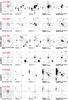 |
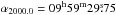
Fig. 1 10″ × 10″ cut-outs of our z> 4 COSMOS SMGs. Shown are the HST/ACS I-band (rest-frame UV) or the stacked HST/WFC3 bands from CANDELS (PI: S. Faber; if available) overlaid with VLA 1.4 GHz radio continuum contours (levels: 2iσ, where i = 1, 2, 3,..., and σ is the local rms), the Subaru V, r+ and z+ broad band filters as well as a stack of the NIR filters of the UltraVISTA survey (Y,J,H,Ks). Spitzer/IRAC 3.6 μm and MIPS 24 μm contours (starting at 3σ, in steps of 3σ) are overlaid onto each z+ and UltraVISTA image, respectively. Spectroscopic redshifts based on Lyα diagnostics from Keck/DEIMOS observations targeting sources indicated by the large black cross are given in the top left corner of the leftmost panels. |
3. Multi-wavelength properties and data
Herschel PACS/SPIRE photometry for our z> 4 SMG sample.
Sub-mm to radio photometry for our z> 4 SMG sample.
Radio properties of our z> 4 SMG sample.
COSMOS is an imaging and spectroscopic survey of an equatorial 2 deg2 field (Scoville et al. 2007). It provides all ancillary data needed for a detailed interpretation of our z> 4 SMG sample given the deep ground- and space-based photometry in more than 30 bands, from the X-rays to the radio (Scoville et al. 2007). The IR to radio photometric measurements for our SMGs are reported in Tables 2–4, and the multi-wavelength data are described in more detail below.
3.1. X-ray properties
The SMGs in our sample are located in an area of the COSMOS field covered by deep (~160–190 ks) Chandra images, which are part of the C-COSMOS (Elvis et al. 2009) and Chandra COSMOS Legacy surveys (XVP; Civano et al., in prep.). None of our SMGs is detected in X-rays. On the basis of the sensitivity of the above surveys (see Puccetti et al. 2009), the detection limit at the position of the sources is ~3–5 × 10-16 erg cm-2 s-1 in the 0.5−2 keV band, which corresponds to an upper limit on the rest-frame luminosity of 1043.5 erg s-1 in the same band, computed assuming z = 4.5, a power law model with spectral index Γ = 1.4 and Galactic hydrogen column density NH, Gal = 2.6 × 1020 cm-2 and no intrinsic absorption. We also performed an X-ray stacking analysis, which does not yield a detection even for the stacked signal. This sets an upper limit on the X-ray luminosity to 1043.1 erg s-1. We note that this limit is significantly higher than the expected X-ray emission from SMGs (Laird et al. 2010) if their X-ray emission were due only to star formation.
3.2. UV-FIR data
The UV-mid-IR (MIR) photometry is taken from the most recent COSMOS photometric catalog, with UltraVISTA (Y,J,H,Ks) DR1 photometry added (see Smolčić et al. 2012; Ilbert et al. 2013; McCracken et al. 2012; Capak et al. 2007). HST/ACS I-band (rest-frame UV) images are taken from Koekemoer et al. (2007), and, if available, HST/WFC3 images from CANDELS (PI: S. Faber; Grogin et al. 2011; Koekemoer et al. 2011).
To assure the most accurate FIR measurements for our sources, we use deep Photodetector Array Camera and Spectrometer (PACS) 100 and 160 μm and Spectral and Photometric Imaging Receiver (SPIRE) 250, 350 and 500 μm observations of the COSMOS field provided by the Herschel Space Observatory (Pilbratt et al. 2010). The PACS observations were taken as part of the PACS Evolutionary Probe (PEP3; Lutz et al. 2011) guaranteed time key program, while the SPIRE observations were taken as part of the Herschel Multi-tiered Extragalactic Survey (HerMES4; Oliver et al. 2012). We extract the Herschel PACS and SPIRE photometry directly from the maps via a point source function (PSF)-fitting analysis (Magnelli et al. 2013) using as prior positions the interferometric position of our SMGs and, where required, the position of MIPS 24 μm sources blended with our SMGs. The Herschel photometry is presented in Table 2 where we also report the reliability of the Herschel fluxes. We note that we cannot decompose the FIR emission for SMG components separated by ≲1″, and thus for those systems we report the integrated photometry.
3.3. Radio data
The 1.4 GHz (20 cm) radio photometry for our SMGs is taken from the VLA-COSMOS 1.4 GHz Large and Deep Projects (Schinnerer et al. 2007, 2010). These reach an rms of ~7–12 μJy beam-1 over the 2 deg2 COSMOS field. The 20 cm fluxes for our sources are listed in Table 3. Our sources are not detected in the 324 MHz (90 cm) VLA-COSMOS map at  angular resolution (Smolčić et al. 2014), as expected given an rms of 0.5 mJy beam-1 in the 324 MHz map. However, all sources but J1000+0234 are detected in the deep GMRT-COSMOS 325 MHz map (at a resolution of
  and reaching an rms of 70–80 μJy beam-1 around our SMGs; Karim et al., in prep.), and their flux densities (based on the peak flux values) are reported in the last column of Table 3. The reduction and imaging of the GMRT-COSMOS 325 MHz map is described in detail in Karim et al. (in prep.).
We here also use 3 GHz data recently taken with the upgraded, Karl G. Jansky Very Large Array (VLA; VLA-COSMOS 3 GHz Large Project, Smolčić et al., in prep.). The data reduction and imaging of the sub-mosaic of the full COSMOS field is described in detail in Novak et al. (2015). The sub-mosaic is based on 130 h of the observations taken in A- and C-configurations (110 and 20 h, respectively) and contains the pointings (P19, P22, P30, P31, P39, and P44) targeting our six SMGs closest to the pointing phase center. The imaging of the pointings was performed using the CASA task CLEAN using the MFMS option that images the full bandwidth simultaneously (Rau & Cornwell 2011) and simultaneously preserves the best possible resolution ( ) and the best possible rms (~4.5 μJy beam-1) in the map (see Rau & Cornwell 2011, for details). The 3 GHz radio stamps of our SMGs at resolution are shown in Fig. 2. All sources are detected in our 3 GHz radio mosaics. We derive their integrated fluxes using a 2D Gaussian fit to the sources (via the AIPS task JMFIT) and peak fluxes using the AIPS task MAXFIT. The ratio of the integrated and peak fluxes for a given radio source is a direct measure of the extent of the source (e.g., Bondi et al. 2008; Kimball & Ivezić 2008). Based on this, we find that at resolution AzTEC/C159 is clearly resolved, J1000+0234 and AK03 may be marginally resolved, while AzTEC1, AzTEC3, and Vd-17871 remain unresolved. We note that although our analysis suggests extended or multiple-component emission for J1000+0234 and AK03, their integrated fluxes obtained via the AIPS task TVSTAT down to the 2σ level are consistent with their peak fluxes, such that we cannot unambiguously determine whether the sources are really resolved at this resolution. Higher resolution radio imaging is required to unambiguously determine the radio-emitting sizes for these sources. In Table 4 we report the deconvolved 3 GHz sizes of our sources. For all the unresolved sources including the two marginally resolved ones, the total flux is then set equal to the peak brightness, while for AzTEC/C159 we use the AIPS task TVSTAT to infer the total flux within the region outlined by the 2σ contour. The fluxes are reported in Table 3.
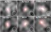 |
Fig. 2 VLA 3 GHz (10 cm) images (~ 3′′ × 3′′ in size) of the studied SMGs. The overlaid red contours show the emission levels starting from 2σ and increasing in steps of 1σ = 4.5μJy beam-1 (the corresponding negative contours levels are shown by dashed contours). The synthesized beam size, |

3.4. Spectroscopic data
All sources in the sample were targeted with DEIMOS on Keck II. In Fig. 3 we show the 1D spectra for AzTEC/C159 and AK03 (the spectra of the remaining sources are given in Capak et al. 2008; Smolčić et al. 2011; Capak et al. 2011; and Karim et al., in prep., for J1000+0234, AzTEC1, AzTEC3, and Vd-17871, respectively). The spectra were taken early 2009 under clear weather conditions and ~1″ seeing and a 4 h integration time split into 30 min exposures using the 830 lines mm-1 grating tilted to 7900 Å and the OG550 blocker. The objects were dithered ±3″ along the slit to remove ghosting. The data reduction was performed via the modified DEEP2 DEIMOS pipeline (see Capak et al. 2008). In both spectra Lyα is clearly detected in emission setting the redshifts to z = 4.747 and z = 4.569 for AK03 and AzTEC/C159, respectively. In Fig. 3 we also show QSO (Croom et al. 2002) and LBG composite spectra constructed by Shapley et al. (2003) from almost 1000 LBGs. The continuum is barely detected for AK03 and AzTEC/C159, and the width of the Lyα line rules out powerful AGN contribution to the SMGs, consistent with their X-ray properties, yet the contribution of a less powerful or obscured AGN cannot be ruled out.
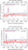 |
Fig. 3 1D Keck II/DEIMOS spectra (red) for AK03 (top panel), and AzTEC/C159 (bottom panel). Also shown are QSO (blue) and LBG (black) composite spectra at the given redshift (labels in the panels). The vertical dashed lines indicate positions of various spectral lines, indicated in the panel. The spectroscopic redshift of the SMG is indicated in the top right corner of each panel. |
4. Spectral energy distributions and derived properties
In this section we analyze the near-UV (NUV) to radio SED properties of our sample of z> 4 SMGs. We self-consistently fit the NUV-mm SEDs of our SMGs using the MAGPHYS model package (Sect. 4.1), we then provide an independent fit of the dust SEDs using only FIR data (Sect. 4.2 ), and finally analyze the radio SEDs of our sources (Sect. 4.3).
4.1. NUV-mm SED fitting
Here we analyze the NUV-mm SEDs of our SMGs via the MAGPHYS (Multi-wavelength Analysis of Galaxy Physical Properties) model package (da Cunha et al. 2008), which self-consistenly balances dust attenuation in the near-IR (NIR) and dust heating in the IR. The UV-NIR SED is modeled based on the Bruzual & Charlot (2003) and Charlot & Fall (2000) stellar population synthesis models. The code then also calculates the absorption of starlight by dust in stellar birth clouds and the diffuse interstellar medium, and computes the SED of the power reradiated by this dust as a sum of three components: i) polycyclic aromatic hydrocarbons (PAHs); ii) hot dust grains (130–250 K) characterizing the MIR continuum; and iii) grains in thermal equilibrium with temperature in the range of 30–60 K.
The MAGPHYS model package provides a library of model spectra that are fit (via a standard χ2 minimization procedure) to the observed SED. Here we use a library optimized for starburst (ULIRG) galaxies (da Cunha et al. 2010). We, however, also utilize a second library, optimized for normal galaxies (da Cunha et al. 2008) in the case of AK03-N and -S as the ULIRG library cannot adequately fit the sources’ SEDs (see below).
We perform the fitting for each of our SMGs using their full NUV-mm photometry (total fluxes de-reddened for foreground Galactic extinction excluding the intermediate band containing the Lyα emission line) extracted at the position of the optical/UltraVISTA counterpart closest to the spectroscopic/mm source (see Fig. 1). The SEDs and the best-fit models for all of our SMGs are shown in Fig. 4, and in Table 5 we list the following parameters from the best-fit models to the observed SEDs for our z> 4 SMGs: the age of the oldest stars in the galaxy giving a formation timescale (tform), total V-band optical depth of the dust seen by young stars in their birth clouds (τV), and the stellar mass (M⋆). For completeness we also list the total dust luminosity (Ldust) calculated over the wavelength range 3–1000 μm, and dust mass (Mdust). However, in the following (Sect. 4.1.2) we independently determine these quantities based on modified blackbody and Draine & Li (2007, hereafter DL07) models, and we adopt the last as the reference value for further analysis. In particular, the IR luminosities derived from the DL07 model refer to the commonly adopted rest-frame wavelength range 8–1000 μm, allowing us to make a direct comparison with SMGs’ IR luminosities reported in the literature (Sect. 5).
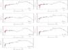 |
Fig. 4 Optical to IR SED fits to our z> 4 SMGs (points for detections, arrows for 4σ upper limits) using the MAGPHYS routine (full black line). |
4.2. FIR properties
To infer the IR luminosities (in the range 8–1000 μm) and dust masses of our z> 4 SMGs we fit their MIR-mm SEDs using an optically thin (τ ≪ 1) modified black-body, and the DL07 dust model. The latter model describes the interstellar dust as a mixture of carbonaceous and amorphous silicate grains and has four free parameters: (i) qPAH, which controls the fraction of dust mass in the form of PAHs; (ii) γ, which controls the fraction of dust mass exposed to a power-law (α = 2) radiation field (relative to the local interstellar value) ranging from Umin to Umax; the rest of the dust mass (i.e., 1-γ) being exposed to a radiation field with a constant intensity Umin; (iii) Umin, which controls the minimum radiation field seen by the dust (Umax is fixed to a value of 106); and (iv) Mdust, which controls the normalization of the SED. Following the prescriptions of DL07, we built a grid of models with different PAH abundances (0.47% <qPAH< 4.6%), values of Umin (0.7–25) and values of γ (0.0–0.3). The best-fit model to each SED, and the corresponding 1σ error is then found via standard χ2 minimization. The fits are shown in Fig. 5 and the results are summarized in Table 6. From the inferred IR luminosities we then further estimate the IR-based SFRs for our z> 4 SMGs, also reported in Table 6, using the standard LIR-to-SFR conversion of Kennicutt (1998), assuming a Chabrier IMF, SFR [M⊙ yr-1] = 10-10LIR [ L⊙ ].
Physical properties of our z> 4 SMG sample derived from the UV-mm SED (using MAGPHYS).
As expected, the Mdust values derived through modified blackbody fits are systematically lower by a factor of ~3–4 than those from the DL07 dust model, because single temperature models do not take into account warmer dust emitting at shorter wavelengths (Magnelli et al. 2012). We also find that in general the dust luminosities and masses derived via MAGPHYS utilizing the NUV-mm SED and those based only on the FIR SED are mostly in reasonable agreement. We note that the results for J1000+0234 are to be taken with caution as the Herschel photometry is affected by confusion, which is reflected in the large error bars. Furthermore, the large difference in dust mass for AK03-S derived via MAGPHYS and IR SED fitting might possibly arise as a result of the high optical thickness assumed in the MAGPHYS model, while the IR modified black-body fitting was performed assuming an optically-thin regime.
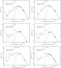 |
Fig. 5 Broadband SEDs of the studied SMGs. The downward pointing arrows denote upper limits to the corresponding flux densities. The red line represents a modified blackbody fit to the FIR-to-mm data points. The blue dashed line is the best fit model, obtained from the superposition of the best fit Draine & Li (2007) model (long-dashed green line) and the stellar black body function (orange dash-dotted line) assuming a temperature of 5000 K, scaled to the residual 24 μm “stellar” flux (i.e., observed 24 μm flux minus that obtained from the DL07 best-fit model). |
4.3. Radio properties
For our z> 4 SMGs at the observed frequencies of 325 MHz, 1.4 GHz, and 3 GHz we are probing rest frame frequencies of approximately 1.8 GHz, 7.7 GHz, and 16.5 GHz (assuming z = 4.5). While the first frequency is expected to be in the region of the spectrum still unaffected by synchrotron self-absorption and energy losses, the latter two frequencies may be affected by energy losses. To account for the possible change in the spectral slope we derive the spectral indices separately at the high and low frequency ends taking the 1.4 GHz data point as the middle, reference point. The results are listed in Table 4.
The synchrotron spectrum for all sources is shown in Fig. 6. Except AzTEC3 and AK03, it is consistent with a single power-law. The steepening of the synchrotron spectrum of AK03 at the high-frequency end may indicate an older age of the electrons exhibiting synchrotron emission. This would be consistent with the formation timescale of ~700 Myr obtained for AK03-S from the UV-mm fitting via MAGPHYS (see Table 5). The synchrotron spectrum of AzTEC 3 flattens at the high-frequency end. As AzTEC 3 is the highest-redshift SMG in our sample (z = 5.298), as given in Table 1, it is possible that the observed radio emission at these high rest-frame frequencies arises from thermal free-free emission (see, e.g., Fig. 1 in Condon 1992).
We further compute the rest-frame monochromatic radio luminosity at 1.4 GHz (L1.4 GHz) using the observed 325 MHz flux (S325 MHz) as it is the closest to 1.4 GHz in the rest-frame, and thus requires the smallest (and hence least uncertain) K-correction: 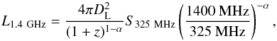 (1)where DL is the luminosity distance, and α is the synchrotron spectral index. Besides using as the synchrotron spectral index the calculated values of
  , we also computed the L1.4 GHz values by assuming that
  . The 1.4 GHz luminosities are reported in Cols. (5) and (6) in Table 4.
Physical properties derived from the IR SED of our z> 4 SMG sample.
 |
Fig. 6 Radio SEDs of the studied SMGs. The dashed lines in each panel represent the spectral slope taking 325 MHz (green point and error-bar) and 1.4 GHz (black point and error-bar; green dashed line) and 1.4 GHz and 3 GHz (blue point and error-bar) data-points (blue dashed line) into account. |
4.4. Summary of SED-derived properties of z ≳ 4 SMGs in COSMOS and comparison with literature
As extensively studied by Dwek et al. (2011), various degeneracies in SED-derived properties exist. We also caution that a debate in the literature exists regarding the optimal model library that gives the most accurate stellar masses for SMGs. Stellar masses have been shown to systematically vary by up to ~0.5 dex if different star formation histories (Michałowski et al. 2010a,b 2012; Hainline et al. 2011) or IMFs (e.g., Dwek et al. 2011) are assumed, and often yield values higher than the inferred dynamical masses (Michałowski et al. 2010a,b). We refer the reader to Dwek et al. and Michałowski et al., for a detailed discussions on possible degeneracies and systematics, and below we summarize the results of the SED modeling performed as described above.
Our SED fitting yields that our z> 4 SMGs contain a dominant young stellar population with ages in the range of ~100–700 Myr, they already have high stellar masses (in the range of 5 × 10¹⁰−4 × 10¹¹M⊙), high dust luminosities (Ldust ~ 1013L⊙), and substantial dust reservoirs (Mdust ~ 109M⊙). If the gas-to-dust mass ratio is ~100, the cold gas masses of our sources are comparable to their stellar masses. As expected, their SFRs are high, ≳400 M⊙ yr-1, and scale up to a few thousand solar masses per year. We note that the derived stellar ages, particularly in the case of faint sources, can suffer from larger uncertainties. For comparison, Wiklind et al. (2014) recently derived a mean (median) stellar age of 0.9 (0.7) Gyr for their sample of SMGs in the CANDELS area of the GOODS-S field. The average IR luminosity we derive, based on the DL07 dust model, is ~1.3 × 10¹³L⊙, while the dust temperatures range from 39 to 48 K. Although large dust masses, warm dust temperatures, and high SFRs are typical for all SMGs (see Casey et al. 2014, for a recent review), the derived properties of our z> 4 SMGs put them at the high end of the distribution of SMG properties. Based on the ALESS SMG sample, Swinbank et al. (2014) find average dust masses of Mdust = (3.6 ± 3) × 108M⊙, IR luminosities of LIR = (3.0 ± 0.3) × 1012L⊙, and SFRs of 300 ± 30M⊙ yr-1, thus systematically lower, by about a factor of three, than the SMGs analyzed here.
Within the uncertainties, our results agree with those previously reported for AzTEC1, AzTEC3, and J1000+0234. For example, Smolčić et al. (2011) found that AzTEC1 is a young (~40–700 Myr old) starburst galaxy with a stellar mass of M⋆ ~ 8 × 10¹⁰M⊙ (scaled to a Chabrier IMF). They furthermore found an IR luminosity for the source of LIR = 2.9 × 10¹³L⊙, and a dust mass of ~1.5 × 10⁹M⊙, in agreement with the results presented here (see Tables 5 and 6). Capak et al. (2011) report values of LIR = (2.2−11) × 1013L⊙, and SFR> 800M⊙ yr-1 for AzTEC3, consistent with our SED modeling results. For J1000+0234, Capak et al. (2008) report a starburst with a stellar mass M⋆> 5.5 × 10¹⁰M⊙, SFR> 550M⊙ yr-1, and LIR = (0.5−2) × 1013L⊙, in agreement with the results presented here. Fitting the total photometry of the source, as done here, they find a >100 Myr old population, consistent with our results. However, deconvolving the various source components they find a young (2–8 Myr) starburst in J1000+0234.
Toft et al. (2014) studied the SED properties of all of our sources except AzTEC/C159. They employed the same methods as in the present work, i.e., MAGPHYS and the DL07 dust model, and the derived SED parameters are mostly very similar to those presented here. We also note that three of our target sources, namely AzTEC1, AzTEC3, and J1000+0234, were part of the recent Herschel study by Huang et al. (2014)5. They only used 250 and 350 μm flux densities (consistent with our values within the errors). Our derived value of LIR for AzTEC1 is within 2σ of that reported by Huang et al. (2014; their Table 4), while our value for AzTEC3 is in very good agreement with theirs. The value for J1000+0234 is also consistent taking into account our large errors. The dust masses of AzTEC1, AzTEC3 and J1000+0234 derived by these authors are also in very good agreement with values inferred here. Our derived dust temperatures, based on the assumption of optically thin emission and fixed dust emissivity index (β = 1.5), are in good agreement with those reported by Huang et al. (2014) in their Table 3. We caution that these assumptions were necessary simplifications to fit the full sample, and note that optical depth effects could matter (see, e.g., Riechers et al. 2013).
5. Discussion
5.1. Infrared-radio correlation
We quantify the IR-radio correlation from the derived IR and radio luminosities in the standard way, i.e., via the q-parameter, defined as:  (2)We note that
  was calculated by integrating over the wavelength range 8–1000 μm. The results are shown, and compared to lower-redshift samples in Fig. 7. Although the associated errors are large (propagated from the average value of the ±-error in
  quoted in Table 6, and from the ±-error in L1.4 GHz), all of our SMGs are offset from the IR-radio relation found in the lower-redshift universe. We used the R program package NADA (Nondetects And Data Analysis for environmental data; Helsel 2005), which is an implementation of the statistical methods provided by the Astronomy Survival Analysis (ASURV; Feigelson & Nelson 1985) package, to take the lower limits to qIR properly into account. This survival analysis yields a mean±standard deviation of ⟨ qIR ⟩ = 1.95 ± 0.26 for our z> 4 SMGs. The inferred median value is 2.02, and the 95% confidence interval 1.75–2.16.
The inferred average qIR value for our SMGs is lower than the qIR value for lower-redshift star forming galaxies (e.g., 2.64 ± 0.02, Bell 2003; 2.57 ± 0.13; Sargent et al. 2010b)6. However, our result is, within the uncertainties, consistent with the on-average lower qIR values inferred for z> 4 SMGs by Murphy (2009; qIR = 2.16 ± 0.28) and Michałowski et al. (2010; qIR = 2.32 ± 0.20).
A lower qIR value (Eq. (2)) can arise either from an underestimation of the IR luminosity or an overestimation of the radio luminosity. The IR luminosities (derived using the DL07 dust model) for our sources in the range of ~6.3 × 10¹²−2.5 × 10¹³L⊙ are unlikely to be underestimated. On the other hand, our 1.4 GHz rest frame radio luminosities have been derived using the 325 MHz observations, very close to 1.4 GHz rest-frame, thus minimizing uncertainties in the calculation (such as an assumed spectral index). This suggests that the deviation is physical. We also note that it is possible that the discrepancy arises as a result of the properties of our limited sample of six spectroscopically confirmed z> 4 SMGs. Thomson et al. (2014) recently derived a median value of qIR = 2.56 ± 0.05 for their sample of 52 ALMA SMGs. The authors also found evidence that the value of qIR changes as a function of source evolutionary stage, and that most of the sources follow the model tracks from Bressan et al. (2002) for evolving starburst galaxies, i.e., the expected q is high (qIR ~ 3) in the very young starburst phase, then it decreases reaching a minimum (qIR ≲ 2) at an age of about 40–50 Myr and finally increases to qIR ~ 2.5 at later times. The low qIR values we derived would then support the idea that the sources are in a relatively early stage of evolution.
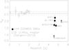 |
Fig. 7 Infrared-radio correlation expressed via the qIR-parameter (Eq. (2)) as a function of redshift. Shown are our z> 4 SMGs (filled circles), and the evolution of the median of the correlation (corrected for systematic effects) for star forming ULIRGs (open squares), adopted from Sargent et al. (2010a). The average qIR = 2.57 ± 0.13 value, found by Sargent et al. (2010b) for galaxies at z< 2, is indicated by the solid line with the dashed lines denoting the errors. For AzTEC3 and J1000+0234 only lower limits to qIR could be derived (marked with arrows). |
5.2. Morphology and sizes of star formation regions
As evident from the HST, and stacked UltraVISTA stamps of our SMGs, shown in Fig. 1, AzTEC1 and AzTEC3 appear compact, while J1000+0234, Vd-17871, and AK03 show signs of clumpiness and multiple components. AzTEC/C159 is a faint source undetected in UltraVISTA YJHKs, but detected in the radio at high significance with clearly resolved 3 GHz emission.
Capak et al. (2008) have demonstrated that all J1000+0234 (compact and extended) components are at the same redshift given that Lyα emission was observed for all of them, and suggested that the components were merging. CO observations of J1000+0234 independently suggest the source is in the process of merging (Schinnerer et al. 2008). Karim et al. (in prep.) have shown that the two components of Vd-17871 lie at comparable spectroscopic redshifts, implying that they are associated and perhaps merging. Based on photometric redshift the same is inferred for AK03-S (Sect. 2). Thus, our sample consists of approximately equal number of compact and clumpy systems, consistent with the idea that SMGs form a morphologically heterogenous sample (e.g., Hayward et al. 2012). It is also possible to see mergers at different stages, for example before or after the coalescence process when regular disk-like geometry is not expected (cf. Targett et al. 2011, 2013). For comparison, Tasca et al. (2014) found that about 20% of star forming galaxies with stellar masses of a few times 1010 M⊙ are involved in major mergers. Based on ALMA data Riechers et al. (2014) find that AzTEC3 is likely to be a merger.
We have made use of our 3 GHz VLA-COSMOS observations at a resolution of  to infer the sizes of the star forming regions in our SMGs (assuming that the 3 GHz emission is due to star formation processes). As evident from Fig. 2 none of the sources shows several radio-emitting components. We find AzTEC/C159 to be clearly resolved at 3 GHz and estimate a deconvolved size of the source (FWHM) at 3 GHz of
  or 6.2 × 3.0 kpc. We find that J1000+0234 and AK03 may be marginally resolved, and their deconvolved sizes (FWHM) are
  and
and  , respectively, corresponding to 6.3 × 4.6 kpc (J1000+0234) and 3.9 × 2.6 kpc (AK03). The remaining sources are unresolved at a resolution of
  setting upper limits on their star formation region sizes (FWHM) to ≤4.6 kpc (AzTEC1), ≤4.3 kpc (AzTEC3), and ≤4.6 kpc (Vd-17871). We note that high-resolution SMA 890 μm continuum and ALMA [ C ii ] measurements of AzTEC1 and AzTEC3, respectively, set an upper limit of the star formation region size of FWHM ≤ 1.3 kpc for AzTEC 1, and 3.9 kpc for AzTEC3 (Younger et al. 2008; Riechers et al. 2010, 2014). Based on these radio and (sub-)mm measurements, we estimate the average size of the star star formation regions of our z> 4 SMGs using the ASURV survival analysis. This yields a mean major axis of
  and minor axis of
  for our sources, and it roughly corresponds to a size of 4.1 × 2.3 kpc2 (assuming z = 4.5). Considering J1000+0234 and AK03 unresolved, the mean major axis decreases to
  . We note that the NIR effective radii derived by Toft et al. (2014) for AzTEC1 and –3 (<2.6 and <2.4 kpc), J1000+0234 (3.7 ± 0.2 kpc), and AK03 (1.6 ± 0.6 kpc) agree well with the above radio FWHM sizes. The sizes inferred here are in agreement with the sizes inferred for lower-redshift SMGs, but are larger than the sizes of local ULIRGs (e.g., Chapman et al. 2004; Tacconi et al. 2006; Rujopakarn et al. 2011; Simpson et al. 2014b). In their recent ALMA band-7 continuum follow-up of a sample of SCUBA-2 detected SMGs in the UDS field, Simpson et al. (2014b) determine an average extent of FWHM ~ 0.3′′. While they report average 1.4 GHz radio continuum sizes that are about twice as large, the cold dust emitting region probed by their 870 μm continuum observations appears to be consistent with the lower bound we derive on average from our high resolution VLA radio data. Whether the average size of the dust emitting region of our specifically z> 4 selected sources is significantly smaller, as found for the Simpson et al. (2014) SMG sample, remains to be clarified based on adequately high resolution interferometric follow-up.
5.3. Relationship between the IR luminosity and dust temperature
Previous studies of populations of infrared-luminous galaxies out to high redshift (including SMGs) have found a relation between dust temperature (Tdust) and IR luminosity (LIR), such that, on average, Tdust increases with LIR (e.g., Chapman et al. 2005; Magnelli et al. 2012; Symeonidis et al. 2013; see also Swinbank et al. 2014). The scatter in this relation strongly depends on the wavelength selection (e.g., Magnelli et al. 2012), but there appears to be a trend for SMGs to have higher LIR than nearby/low-z ULIRGs at the same Tdust (expressed by some authors as a lower Tdust at a given LIR)7. Assuming that the same Tdust can only be maintained by the same IR luminosity surface densities (ΣIR), this trend likely indicates more spatially-extended IR-emitting regions in SMGs, at a given Tdust. This picture is consistent with the large, typically 2–4 kpc sizes of SMGs observed at submillimeter wavelengths (e.g., Tacconi et al. 2008), which indicate wide-spread star formation fueled by large quantities of cold gas (e.g., Ivison et al. 2011; Riechers et al. 2011). Like other star forming galaxy populations at similar redshifts (e.g., Daddi et al. 2008, 2010; Tacconi et al. 2010, 2013), SMGs also appear to have higher gas mass fractions than nearby starbursts and ULIRGs (e.g., Riechers et al. 2011; Ivison et al. 2011), and thus, higher gas and dust masses than nearby galaxies at the same LIR. This is consistent with the interpretation of the Tdust–LIR relation by Symeonidis et al. (2013), but we note that the relation to the dust mass is likely indirect at best, since the dust in SMGs is likely optically thick at the peak wavelengths that are most decisive for the estimates of Tdust and LIR.
To put the derived properties of our z> 4 SMGs in context of the general population of IR galaxies, in Fig. 8 we show dust temperature versus IR luminosity for our SMGs, and compare this to various IR- and submm-selected samples presented in the literature: the locus of local (z ≲ 0.1) IRAS-selected IR galaxies (Symeonidis et al. 2013 and references therein), Herschel-selected 0.1 <z< 2 IR galaxies (Symeonidis et al. 2013), a compilation of SMGs from various fields (Magnelli et al. 2012), the SMG sample from Chapman et al. (2005), and the ALESS SMG sample (Swinbank et al. 2014).
Our z> 4 SMGs fall in the scatter of the z ~ 2 SMG sample from Chapman et al. (2005; albeit towards the high-LIR end because of their initial selection), consistent with their sizes of a few kpc measured at radio and/or submillimeter wavelengths. Some of the z> 4 SMGs fall towards the high-Tdust end, consistent with the different K-correction at higher redshifts in the (sub)millimeter bands (e.g., Chapman et al. 2005 – maybe also add Blain et al. 2004-ish). These systems consistently show high IR luminosity and SFR surface densitites (e.g., Younger et al. 2008; Riechers et al. 2014), approaching those of so-called “maximum starbursts” (e.g., Scoville 2003; Thompson et al. 2005). Our inferred, highest dust masses are also consistent with this picture.
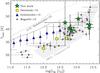 |
Fig. 8 Dust temperature plotted as a function of IR luminosity. The values obtained for our SMGs are shown with green star symbols. The other symbols and lines mark values and correlations from the quoted reference studies (see text for details). The shaded region illustrates the correlation found by Chapman et al. (2005) for their sample of SMGs. |
6. Summary
To constrain the physical characteristics of high-redshift SMGs, we have carried out a study of a sample of six SMGs in the COSMOS field with spectroscopically confirmed redshifts z> 4 (the average z being 4.7). Our main findings are summarized as follows:
-
Based on new, VLA-COSMOS 3 GHz radio dataat resolutionof
we estimate the sizes of the star formation regions of our z> 4 SMGs. Using additional millimetric imaging from literature for AzTEC1 and AzTEC3 and taking limits into account using the ASURV package we estimate a mean size of  or about 4.1 × 2.3 kpc2 (assuming z = 4.5) for our z> 4 SMGs (or lower if we take the two possibly resolved SMGs, J1000+0234 and AK03, as unresolved). These values are consistent with those derived for lower-redshift SMGs, yet higher than for local ULIRGs.
 -
The SED analysis performed with the MAGPHYS code suggests that the stellar masses in our SMGs are in the range M⋆ ~ 0.5−3.9 × 10¹¹ M⊙. The resulting dust masses and luminosities are found to be ~3.6 × 10⁸−5.6 × 10¹⁰ M⊙ and ~0.14−3.4 × 10¹³L⊙. The inferred ages of the oldest stars in these systems range from about 100 to ~700 Myr, with an average age of ~280 Myr, and with 5 out of 6 SMGs having estimated ages smaller than ~200 Myr. The dust properties were also determined through fitting the SEDs with modified blackbody curves and employing the Draine & Li (2007) dust model. The former yields the values Mdust ~ 0.3−1.3 × 10⁹ M⊙ and LIR ~ 4 × 10¹¹−2.3 × 10¹³L⊙, while the latter method gives Mdust ~ 1−5 × 10⁹ M⊙ and LIR ~ 0.5−2.5 × 10¹³L⊙. The derived dust temperatures, ~39–48 K, are relatively warm compared to lower-redshift, but lower LIR SMGs. Finally, the star formation rates we determine, ~450–2500 M⊙ yr-1, conform with the idea that the sources are very dusty starburst galaxies.
-
Using new 325 MHz (GMRT), 1.4 GHz (VLA), and 3 GHz (VLA) data we derive the 1.4 GHz luminosities for our SMGs, found to be in the range of about 1025 W Hz-1 up to possibly 2.4 × 1025 W Hz-1 (when using spectral indices drawn from 0.325 and 1.4 GHz fluxes).
-
Using the derived (Draine & Li 2007) IR and 1.4 GHz luminosities we investigate the IR-radio correlation for our SMGs, as quantified by the q parameter. We find it to be lower for our z> 4 SMGs (⟨ q ⟩ = 1.95 ± 0.26) compared to that found for lower-redshift galaxies. This may be due to selection effects and supports the idea that the sources are in a relatively early stage of evolution.
-
Inspection of the relationship between IR luminosity and dust temperature shows that our SMGs lie at the high end of the correlation, consistent with an extrapolation of the high-redshift LIR−Tdust relation previously inferred for Herschel-selected 0.1 <z< 2 galaxies. Thus, we conclude that at fixed LIR the cold dust LIR − Tdust of high-redshift SMGs is likely due to more extended star formation regions in high-redshift SMGs relative to local ULIRGs and higher dust masses in high-redshift galaxies, compared to lower-redshift SMG samples, as has been previously suggested.
In summary, we find that our sample consists of a fair mix of compact and clumpy systems, consistent with the idea that (sub-)mm galaxy identification may select physically heterogeneous samples of galaxies. The compact appearance might be an indication of a merger remnant rather than a regular star forming disk galaxy. Thus, further studies are required to examine how z> 4 SMGs are related to z< 3 SMGs, and other populations, such as massive ellipticals at z ~ 2 and locally, as well as to quantify the role played by SMGs in galaxy formation and evolution.
Five SMGs in their sample overlap with the sample analyzed by Michałowski et al. (2010), and three with the sample presented here (AzTEC 1, AzTEC 3, and J1000+0234).
All the sources in the paper by Scott et al. (2008) were identified from the central 0.15 deg2 area with a uniform sensitivity of ~1.3 mJy beam-1.
The SMG J1000+0234 is called Capak4.55 in Huang et al. (2014).
As in the present paper, the IR luminosities in the reference studies were calculated over the wavelength range 8–1000 μm.
These populations only overlap at the lower-LIR end of SMGs.
Acknowledgments
We thank the referee for insightful comments on the manuscript. This research was funded by the European Union’s Seventh Frame-work program under grant agreement 337595 (ERC Starting Grant, “CoSMass”). A.K. acknowledges support by the Collaborative Research Council 956, sub-project A1, funded by the Deutsche Forschungsgemeinschaft (DFG). The Dark Cosmology Centre is funded by the Danish National Research Foundation. The National Radio Astronomy Observatory is a facility of the National Science Foundation operated under cooperative agreement by Associated Universities, Inc.
References
- Aihara, H., Allen de Prieto, C., An, D., et al. 2011, ApJS, 193, 29 [NASA ADS] [CrossRef] [Google Scholar]
- Alberts, S., Wilson, G. W., Lu, Y., et al. 2013, MNRAS, 431, 194 [NASA ADS] [CrossRef] [Google Scholar]
- Aravena, M., Bertoldi, F., Carilli, C., et al. 2010, ApJ, 708, L36 [NASA ADS] [CrossRef] [Google Scholar]
- Aretxaga, I., Wilson, G. W., Aguilar, E., et al. 2011, MNRAS, 415, 3831 [NASA ADS] [CrossRef] [Google Scholar]
- Barger, A. J., Cowie, L. L., Sanders, D. B., et al. 1998, Nature, 394, 248 [NASA ADS] [CrossRef] [Google Scholar]
- Barger, A. J., Wang, W.-H., Cowie, L. L., et al. 2012, ApJ, 761, 89 [Google Scholar]
- Bell, E. F. 2003, ApJ, 586, 794 [Google Scholar]
- Bertoldi, F., Carilli, C., Aravena, M., et al. 2007, ApJS, 172, 132 [NASA ADS] [CrossRef] [Google Scholar]
- Biggs, A. D., Ivison, R. J., Ibar, E., et al. 2011, MNRAS, 413, 2314 [Google Scholar]
- Blain, A. W., Smail, I., Ivison, R. J., Kneib, J.-P., & Frayer, D. T. 2002, Phys. Rep., 369, 111 [NASA ADS] [CrossRef] [Google Scholar]
- Bondi, M., Ciliegi, P., Schinnerer, E., et al. 2008, ApJ, 681, 1129 [NASA ADS] [CrossRef] [Google Scholar]
- Botzler, C. S., Snigula, J., Bender, R., & Hopp, U. 2004, MNRAS, 349, 425 [NASA ADS] [CrossRef] [Google Scholar]
- Bressan, A., Silva, L., & Granato, G. L. 2002, A&A, 392, 377 [NASA ADS] [CrossRef] [EDP Sciences] [Google Scholar]
- Bruzual, G., & Charlot, S. 2003, MNRAS, 344, 1000 [NASA ADS] [CrossRef] [Google Scholar]
- Capak, P., Aussel, H., Ajiki, M., et al. 2007, ApJS, 172, 99 [NASA ADS] [CrossRef] [Google Scholar]
- Capak, P., Carilli, C. L., Lee, N., et al. 2008, ApJ, 681, L53 [Google Scholar]
- Capak, P. L., Riechers, D., Scoville, N. Z., et al. 2011, Nature, 470, 233 [Google Scholar]
- Carilli, C. L., Hodge, J., Walter, F., et al. 2011, ApJ, 739, L33 [NASA ADS] [CrossRef] [Google Scholar]
- Casey, C. M., Chen, C.-C., Cowie, L. L., et al. 2013, MNRAS, 436, 1919 [NASA ADS] [CrossRef] [Google Scholar]
- Casey, C. M., Narayanan, D., & Cooray, A. 2014, Phys. Rep., 541, 45 [NASA ADS] [CrossRef] [Google Scholar]
- Chabrier, G. 2003, PASP, 115, 763 [NASA ADS] [CrossRef] [Google Scholar]
- Chapman, S. C., Smail, I., Windhorst, R., Muxlow, T., & Ivison, R. J. 2004, ApJ, 611, 732 [NASA ADS] [CrossRef] [Google Scholar]
- Chapman, S. C., Blain, A. W., Smail, I., & Ivison, R. J. 2005, ApJ, 622, 772 [NASA ADS] [CrossRef] [Google Scholar]
- Charlot, S., & Fall, S. M. 2000, ApJ, 539, 718 [NASA ADS] [CrossRef] [Google Scholar]
- Combes, F., Rex, M., Rawle, T. D., et al. 2012, A&A, 538, L4 [NASA ADS] [CrossRef] [EDP Sciences] [Google Scholar]
- Condon, J. J. 1992, ARA&A, 30, 575 [NASA ADS] [CrossRef] [MathSciNet] [Google Scholar]
- Condon, J. J., Cotton, W. D., Fomalont, E. B., et al. 2012, ApJ, 758, 23 [NASA ADS] [CrossRef] [Google Scholar]
- Coppin, K. E. K., Smail, I., Alexander, D. M., et al. 2009, MNRAS, 395, 1905 [NASA ADS] [CrossRef] [Google Scholar]
- Cox, P., Krips, M., Neri, R., et al. 2011, ApJ, 740, 63 [NASA ADS] [CrossRef] [Google Scholar]
- Croom, S. M., Rhook, K., Corbett, E. A., et al. 2002, MNRAS, 337, 275 [NASA ADS] [CrossRef] [Google Scholar]
- da Cunha, E., Charlot, S., & Elbaz, D. 2008, MNRAS, 388, 1595 [NASA ADS] [CrossRef] [Google Scholar]
- da Cunha, E., Charmandaris, V., Díaz-Santos, T., et al. 2010, A&A, 523, A78 [NASA ADS] [CrossRef] [EDP Sciences] [Google Scholar]
- Daddi, E., Dannerbauer, H., Elbaz, D., et al. 2008, ApJ, 673, L21 [NASA ADS] [CrossRef] [Google Scholar]
- Daddi, E., Dannerbauer, H., Stern, D., et al. 2009a, ApJ, 694, 1517 [Google Scholar]
- Daddi, E., Dannerbauer, H., Krips, M., et al. 2009b, ApJ, 695, L176 [NASA ADS] [CrossRef] [Google Scholar]
- De Breuck, C., Williams, R. J., Swinbank, M., et al. 2014, A&A, 565, A59 [NASA ADS] [CrossRef] [EDP Sciences] [Google Scholar]
- Dowell, C. D., Conley, A., Glenn, J., et al. 2014, ApJ, 780, 75 [NASA ADS] [CrossRef] [Google Scholar]
- Draine, B. T., & Li, A. 2007, ApJ, 657, 810 (DL07) [NASA ADS] [CrossRef] [Google Scholar]
- Dwek, E., Staguhn, J. G., Arendt, R. G., et al. 2011, ApJ, 738, 36 [NASA ADS] [CrossRef] [Google Scholar]
- Elvis, M., Civano, F., Vignali, C., et al. 2009, ApJS, 184, 158 [NASA ADS] [CrossRef] [Google Scholar]
- Engel, H., Tacconi, L. J., Davies, R. I., et al. 2010, ApJ, 724, 233 [NASA ADS] [CrossRef] [Google Scholar]
- Feigelson, E. D., & Nelson, P. I. 1985, ApJ, 293, 192 [NASA ADS] [CrossRef] [Google Scholar]
- Grogin, N. A., Kocevski, D. D., Faber, S. M., et al. 2011, ApJS, 197, 35 [NASA ADS] [CrossRef] [Google Scholar]
- Hainline, L. J., Blain, A. W., Smail, I., et al. 2011, ApJ, 740, 96 [NASA ADS] [CrossRef] [Google Scholar]
- Hayward, C. C., Jonsson, P., Kereš, D., et al. 2012, MNRAS, 424, 951 [NASA ADS] [CrossRef] [Google Scholar]
- Helsel, D. R. 2005, Nondetects And Data Analysis: Statistics for Censored Environmental Data (New York: John Wiley and Sons) [Google Scholar]
- Hickox, R. C., Wardlow, J. L., Smail, I., et al. 2012, MNRAS, 421, 284 [NASA ADS] [Google Scholar]
- Hodge, J. A., Carilli, C. L., Walter, F., et al. 2012, ApJ, 760, 11 [Google Scholar]
- Hodge, J. A., Karim, A., Smail, I., et al. 2013, ApJ, 768, 91 [NASA ADS] [CrossRef] [Google Scholar]
- Huang, J.-S., Rigopoulou, D., Magdis, G., et al. 2014, ApJ, 784, 52 [NASA ADS] [CrossRef] [Google Scholar]
- Huynh, M. T., Norris, R. P., Coppin, K. E. K., et al. 2013, MNRAS, 431, L88 [NASA ADS] [CrossRef] [Google Scholar]
- Ilbert, O., Capak, P., Salvato, M., et al. 2009, ApJ, 690, 1236 [NASA ADS] [CrossRef] [Google Scholar]
- Ilbert, O., McCracken, H. J., Le Févre, O., et al. 2013, A&A, 556, A55 [NASA ADS] [CrossRef] [EDP Sciences] [Google Scholar]
- Ivison, R. J., Papadopoulos, P. P., Smail, I., et al. 2011, MNRAS, 412, 1913 [NASA ADS] [CrossRef] [Google Scholar]
- Karim, A., Swinbank, A. M., Hodge, J. A., et al. 2013, MNRAS, 432, 2 [NASA ADS] [CrossRef] [Google Scholar]
- Kennicutt, R. C., Jr. 1998, ARA&A, 36, 189 [Google Scholar]
- Kim, R. S. J., Kepner, J. V., Postman, M., et al. 2002, AJ, 123, 20 [NASA ADS] [CrossRef] [Google Scholar]
- Kimball, A. E., & Ivezić, Ž. 2008, AJ, 136, 684 [NASA ADS] [CrossRef] [Google Scholar]
- Koekemoer, A. M., Aussel, H., Calzetti, D., et al. 2007, ApJS, 172, 196 [NASA ADS] [CrossRef] [Google Scholar]
- Koekemoer, A. M., Faber, S. M., Ferguson, H. C., et al. 2011, ApJS, 197, 36 [NASA ADS] [CrossRef] [Google Scholar]
- Kovács, A., Chapman, S. C., Dowell, C. D., et al. 2006, ApJ, 650, 592 [NASA ADS] [CrossRef] [Google Scholar]
- Knudsen, K. K., Kneib, J.-P., Richard, J., Petitpas, G., & Egami, E. 2010, ApJ, 709, 210 [NASA ADS] [CrossRef] [Google Scholar]
- Krolik, J. H., & Chen, W. 1991, AJ, 102, 1659 [NASA ADS] [CrossRef] [Google Scholar]
- Laird, E. S., Nandra, K., Pope, A., & Scott, D. 2010, MNRAS, 401, 2763 [NASA ADS] [CrossRef] [Google Scholar]
- Le Fèvre, O., Tasca, L. A. M., Cassata, P., et al. 2015, A&A, 576, A79 [NASA ADS] [CrossRef] [EDP Sciences] [Google Scholar]
- Lilly, S. J., Le Fèvre, O., Renzini, A., et al. 2007, ApJS, 172, 70 [NASA ADS] [CrossRef] [Google Scholar]
- Lilly, S. J., Le Brun, V., Maier, C., et al. 2009, ApJS, 184, 218 [Google Scholar]
- Lutz, D., Poglitsch, A., Altieri, B., et al. 2011, A&A, 532, A90 [NASA ADS] [CrossRef] [EDP Sciences] [Google Scholar]
- Magnelli, B., Lutz, D., Santini, P., et al. 2012, A&A, 539, A155 [NASA ADS] [CrossRef] [EDP Sciences] [Google Scholar]
- Magnelli, B., Popesso, P., Berta, S., et al. 2013, A&A, 553, A132 [NASA ADS] [CrossRef] [EDP Sciences] [Google Scholar]
- McCracken, H. J., Milvang-Jensen, B., Dunlop, J., et al. 2012, A&A, 544, A156 [NASA ADS] [CrossRef] [EDP Sciences] [Google Scholar]
- Michałowski, M., Hjorth, J., & Watson, D. 2010a, A&A, 514, A67 [NASA ADS] [CrossRef] [EDP Sciences] [Google Scholar]
- Michałowski, M. J., Watson, D., & Hjorth, J. 2010b, ApJ, 712, 942 [NASA ADS] [CrossRef] [Google Scholar]
- Miley, G., & De Breuck, C. 2008, A&ARv, 15, 67 [NASA ADS] [CrossRef] [Google Scholar]
- Murphy, E. J. 2009, ApJ, 706, 482 [NASA ADS] [CrossRef] [Google Scholar]
- Narayanan, D., Hayward, C. C., Cox, T. J., et al. 2010, MNRAS, 401, 1613 [NASA ADS] [CrossRef] [MathSciNet] [Google Scholar]
- Novak, M., Smolčić, V., Civano, F., et al. 2015, MNRAS, 447, 1282 [NASA ADS] [CrossRef] [Google Scholar]
- Oliver, S. J., Bock, J., Altieri, B., et al. 2012, MNRAS, 424, 1614 [NASA ADS] [CrossRef] [EDP Sciences] [Google Scholar]
- Onodera, M., Daddi, E., Gobat, R., et al. 2010, ApJ, 715, L6 [NASA ADS] [CrossRef] [Google Scholar]
- Pilbratt, G. L., Riedinger, J. R., Passvogel, T., et al. 2010, A&A, 518, L1 [CrossRef] [EDP Sciences] [Google Scholar]
- Prescott, M. K. M., Impey, C. D., Cool, R. J., & Scoville, N. Z. 2006, ApJ, 644, 100 [NASA ADS] [CrossRef] [Google Scholar]
- Puccetti, S., Vignali, C., Cappelluti, N., et al. 2009, ApJS, 185, 586 [NASA ADS] [CrossRef] [Google Scholar]
- Ramella, M., Boschin, W., Fadda, D., & Nonino, M. 2001, A&A, 368, 776 [NASA ADS] [CrossRef] [EDP Sciences] [Google Scholar]
- Rau, U., & Cornwell, T. J. 2011, A&A, 532, A71 [NASA ADS] [CrossRef] [EDP Sciences] [Google Scholar]
- Riechers, D. A., Capak, P. L., Carilli, C. L., et al. 2010, ApJ, 720, L131 [NASA ADS] [CrossRef] [Google Scholar]
- Riechers, D. A., Hodge, J., Walter, F., Carilli, C. L., & Bertoldi, F. 2011, ApJ, 739, L31 [NASA ADS] [CrossRef] [Google Scholar]
- Riechers, D. A., Bradford, C. M., Clements, D. L., et al. 2013, Nature, 496, 329 [Google Scholar]
- Riechers, D. A., Carilli, C. L., Capak, P. L., et al. 2014, ApJ, 796, 84 [NASA ADS] [CrossRef] [Google Scholar]
- Rujopakarn, W., Rieke, G. H., Eisenstein, D. J., & Juneau, S. 2011, ApJ, 726, 93 [NASA ADS] [CrossRef] [Google Scholar]
- Salpeter, E. E. 1955, ApJ, 121, 161 [Google Scholar]
- Salvato, M., Hasinger, G., Ilbert, O., et al. 2009, ApJ, 690, 1250 [CrossRef] [Google Scholar]
- Sargent, M. T., Schinnerer, E., Murphy, E., et al. 2010a, ApJS, 186, 341 [NASA ADS] [CrossRef] [Google Scholar]
- Sargent, M. T., Schinnerer, E., Murphy, E., et al. 2010b, ApJ, 714, L190 [NASA ADS] [CrossRef] [Google Scholar]
- Schinnerer, E., Smolčić, V., Carilli, C. L., et al. 2007, ApJS, 172, 46 [NASA ADS] [CrossRef] [Google Scholar]
- Schinnerer, E., Carilli, C. L., Capak, P., et al. 2008, ApJ, 689, L5 [Google Scholar]
- Schinnerer, E., Sargent, M. T., Bondi, M., et al. 2010, ApJS, 188, 384 [NASA ADS] [CrossRef] [Google Scholar]
- Scott, K. S., Austermann, J. E., Perera, T. A., et al. 2008, MNRAS, 385, 2225 [NASA ADS] [CrossRef] [Google Scholar]
- Scoville, N. 2003, JKAS, 36, 167 [Google Scholar]
- Scoville, N., Aussel, H., Brusa, M., et al. 2007, ApJS, 172, 1 [NASA ADS] [CrossRef] [Google Scholar]
- Shapley, A. E., Steidel, C. C., Pettini, M., & Adelberger, K. L. 2003, ApJ, 588, 65 [NASA ADS] [CrossRef] [Google Scholar]
- Simpson, J. M., Swinbank, A. M., Smail, I., et al. 2014a, ApJ, 788, 125 [Google Scholar]
- Simpson, J. M., Smail, I., Swinbank, A. M., et al. 2014b, ApJ, submitted [arXiv:1411.5025] [Google Scholar]
- Smolčić, V., Schinnerer, E., Finoguenov, A., et al. 2007, ApJS, 172, 295 [NASA ADS] [CrossRef] [Google Scholar]
- Smolčić, V., Capak, P., Ilbert, O., et al. 2011, ApJ, 731, L27 [NASA ADS] [CrossRef] [Google Scholar]
- Smolčić, V., Aravena, M., Navarrete, F., et al. 2012, A&A, 548, A4 [NASA ADS] [CrossRef] [EDP Sciences] [Google Scholar]
- Smolčić, V., Ciliegi, P., Jelić, V., et al. 2014, MNRAS, 443, 2590 [NASA ADS] [CrossRef] [Google Scholar]
- Springel, V., Di Matteo, T., & Hernquist, L. 2005, ApJ, 620, L79 [NASA ADS] [CrossRef] [Google Scholar]
- Swinbank, A. M., Simpson, J. M., Smail, I., et al. 2014, MNRAS, 438, 1267 [Google Scholar]
- Symeonidis, M., Vaccari, M., Berta, S., et al. 2013, MNRAS, 431, 2317 [NASA ADS] [CrossRef] [Google Scholar]
- Tacconi, L. J., Neri, R., Chapman, S. C., et al. 2006, ApJ, 640, 228 [NASA ADS] [CrossRef] [Google Scholar]
- Tacconi, L. J., Genzel, R., Smail, I., et al. 2008, ApJ, 680, 246 [NASA ADS] [CrossRef] [PubMed] [Google Scholar]
- Tacconi, L. J., Genzel, R., Neri, R., et al. 2010, Nature, 463, 781 [Google Scholar]
- Tacconi, L. J., Neri, R., Genzel, R., et al. 2013, ApJ, 768, 74 [Google Scholar]
- Targett, T. A., Dunlop, J. S., McLure, R. J., et al. 2011, MNRAS, 412, 295 [NASA ADS] [CrossRef] [Google Scholar]
- Targett, T. A., Dunlop, J. S., Cirasuolo, M., et al. 2013, MNRAS, 432, 2012 [NASA ADS] [CrossRef] [Google Scholar]
- Tasca, L. A. M., Le Fèvre, O., López-Sanjuan, C., et al. 2014, A&A, 565, A10 [NASA ADS] [CrossRef] [EDP Sciences] [Google Scholar]
- Thompson, T. A., Quataert, E., & Murray, N. 2005, ApJ, 630, 167 [NASA ADS] [CrossRef] [Google Scholar]
- Thomson, A. P., Ivison, R. J., Simpson, J. M., et al. 2014, MNRAS, 442, 577 [NASA ADS] [CrossRef] [Google Scholar]
- Toft, S., Smolčić, V., Magnelli, B., et al. 2014, ApJ, 782, 68 [NASA ADS] [CrossRef] [Google Scholar]
- Trump, J. R., Impey, C. D., McCarthy, P. J., et al. 2007, ApJS, 172, 383 [NASA ADS] [CrossRef] [Google Scholar]
- Walter, F., Decarli, R., Carilli, C., et al. 2012, Nature, 486, 233 [NASA ADS] [CrossRef] [Google Scholar]
- Wardlow, J. L., Smail, I., Coppin, K. E. K., et al. 2011, MNRAS, 415, 1479 [NASA ADS] [CrossRef] [Google Scholar]
- Weiß, A., Kovács, A., Coppin, K., et al. 2009, ApJ, 707, 1201 [NASA ADS] [CrossRef] [Google Scholar]
- Weiß, A., De Breuck, C., Marrone, D. P., et al. 2013, ApJ, 767, 88 [NASA ADS] [CrossRef] [Google Scholar]
- Wiklind, T., Conselice, C. J., Dahlen, T., et al. 2014, ApJ, 785, 111 [NASA ADS] [CrossRef] [Google Scholar]
- Younger, J. D., Fazio, G. G., Huang, J.-S., et al. 2007, ApJ, 671, 1531 [Google Scholar]
- Younger, J. D., Fazio, G. G., Wilner, D. J., et al. 2008, ApJ, 688, 59 [NASA ADS] [CrossRef] [Google Scholar]
- Yun, M. S., Reddy, N. A., & Condon, J. J. 2001, ApJ, 554, 803 [NASA ADS] [CrossRef] [Google Scholar]
- Zavala, J. A., Aretxaga, I., & Hughes, D. H. 2014, MNRAS, 443, 2384 [NASA ADS] [CrossRef] [PubMed] [Google Scholar]
All Tables
Physical properties of our z> 4 SMG sample derived from the UV-mm SED (using MAGPHYS).
All Figures
|
Fig. 1 10″ × 10″ cut-outs of our z> 4 COSMOS SMGs. Shown are the HST/ACS I-band (rest-frame UV) or the stacked HST/WFC3 bands from CANDELS (PI: S. Faber; if available) overlaid with VLA 1.4 GHz radio continuum contours (levels: 2iσ, where i = 1, 2, 3,..., and σ is the local rms), the Subaru V, r+ and z+ broad band filters as well as a stack of the NIR filters of the UltraVISTA survey (Y,J,H,Ks). Spitzer/IRAC 3.6 μm and MIPS 24 μm contours (starting at 3σ, in steps of 3σ) are overlaid onto each z+ and UltraVISTA image, respectively. Spectroscopic redshifts based on Lyα diagnostics from Keck/DEIMOS observations targeting sources indicated by the large black cross are given in the top left corner of the leftmost panels. |
| In the text | |
|
Fig. 2 VLA 3 GHz (10 cm) images (~ 3′′ × 3′′ in size) of the studied SMGs. The overlaid red contours show the emission levels starting from 2σ and increasing in steps of 1σ = 4.5μJy beam-1 (the corresponding negative contours levels are shown by dashed contours). The synthesized beam size, |
| In the text | |
|
Fig. 3 1D Keck II/DEIMOS spectra (red) for AK03 (top panel), and AzTEC/C159 (bottom panel). Also shown are QSO (blue) and LBG (black) composite spectra at the given redshift (labels in the panels). The vertical dashed lines indicate positions of various spectral lines, indicated in the panel. The spectroscopic redshift of the SMG is indicated in the top right corner of each panel. |
| In the text | |
|
Fig. 4 Optical to IR SED fits to our z> 4 SMGs (points for detections, arrows for 4σ upper limits) using the MAGPHYS routine (full black line). |
| In the text | |
|
Fig. 5 Broadband SEDs of the studied SMGs. The downward pointing arrows denote upper limits to the corresponding flux densities. The red line represents a modified blackbody fit to the FIR-to-mm data points. The blue dashed line is the best fit model, obtained from the superposition of the best fit Draine & Li (2007) model (long-dashed green line) and the stellar black body function (orange dash-dotted line) assuming a temperature of 5000 K, scaled to the residual 24 μm “stellar” flux (i.e., observed 24 μm flux minus that obtained from the DL07 best-fit model). |
| In the text | |
|
Fig. 6 Radio SEDs of the studied SMGs. The dashed lines in each panel represent the spectral slope taking 325 MHz (green point and error-bar) and 1.4 GHz (black point and error-bar; green dashed line) and 1.4 GHz and 3 GHz (blue point and error-bar) data-points (blue dashed line) into account. |
| In the text | |
|
Fig. 7 Infrared-radio correlation expressed via the qIR-parameter (Eq. (2)) as a function of redshift. Shown are our z> 4 SMGs (filled circles), and the evolution of the median of the correlation (corrected for systematic effects) for star forming ULIRGs (open squares), adopted from Sargent et al. (2010a). The average qIR = 2.57 ± 0.13 value, found by Sargent et al. (2010b) for galaxies at z< 2, is indicated by the solid line with the dashed lines denoting the errors. For AzTEC3 and J1000+0234 only lower limits to qIR could be derived (marked with arrows). |
| In the text | |
|
Fig. 8 Dust temperature plotted as a function of IR luminosity. The values obtained for our SMGs are shown with green star symbols. The other symbols and lines mark values and correlations from the quoted reference studies (see text for details). The shaded region illustrates the correlation found by Chapman et al. (2005) for their sample of SMGs. |
| In the text | |
Current usage metrics show cumulative count of Article Views (full-text article views including HTML views, PDF and ePub downloads, according to the available data) and Abstracts Views on Vision4Press platform.
Data correspond to usage on the plateform after 2015. The current usage metrics is available 48-96 hours after online publication and is updated daily on week days.
Initial download of the metrics may take a while.