| Issue |
A&A
Volume 576, April 2015
|
|
|---|---|---|
| Article Number | A77 | |
| Number of page(s) | 17 | |
| Section | Numerical methods and codes | |
| DOI | https://doi.org/10.1051/0004-6361/201423932 | |
| Published online | 01 April 2015 | |
Molecfit: A general tool for telluric absorption correction
I. Method and application to ESO instruments ⋆,⋆⋆
1 European Southern Observatory, Casilla 19001, Alonso de Cordova 3107 Vitacura, Santiago, Chile
e-mail: asmette@eso.org
2 now at ESA/Space Telescope Science Institute, 3700 San Martin Dr, Baltimore, MD 21218, USA
3 Institute for Astro and Particle Physics, Universität Innsbruck, Technikerstrasse 25, 6020 Innsbruck, Austria
4 Josef-Führer-Straße 33, 80997 München, Germany
5 University of Vienna, Department of Astrophysics, Türkenschanzstr. 17 (Sternwarte), 1180 Vienna, Austria
6 Instituto de Astronomía, Universidad Católica del Norte, Avenida Angamos 0610, Antofagasta, Chile
7 International Graduate School of Science and Engineering, Technische Universität München, Boltzmannstr. 17, 85748 Garching bei München, Germany
8 Universidad de Concepción, Casilla 160-C, Concepción, Chile
9 European Southern Observatory, Karl-Schwarzschild-Strasse 2, 85748 Garching bei München, Germany
Received: 2 April 2014
Accepted: 23 December 2014
Context. The interaction of the light from astronomical objects with the constituents of the Earth’s atmosphere leads to the formation of telluric absorption lines in ground-based collected spectra. Correcting for these lines, mostly affecting the red and infrared region of the spectrum, usually relies on observations of specific stars obtained close in time and airmass to the science targets, therefore using precious observing time.
Aims. We present molecfit, a tool to correct for telluric absorption lines based on synthetic modelling of the Earth’s atmospheric transmission. Molecfit is versatile and can be used with data obtained with various ground-based telescopes and instruments.
Methods. Molecfit combines a publicly available radiative transfer code, a molecular line database, atmospheric profiles, and various kernels to model the instrument line spread function. The atmospheric profiles are created by merging a standard atmospheric profile representative of a given observatory’s climate, of local meteorological data, and of dynamically retrieved altitude profiles for temperature, pressure, and humidity. We discuss the various ingredients of the method, its applicability, and its limitations. We also show examples of telluric line correction on spectra obtained with a suite of ESO Very Large Telescope (VLT) instruments.
Results. Compared to previous similar tools, molecfit takes the best results for temperature, pressure, and humidity in the atmosphere above the observatory into account. As a result, the standard deviation of the residuals after correction of unsaturated telluric lines is frequently better than 2% of the continuum.
Conclusions. Molecfit is able to accurately model and correct for telluric lines over a broad range of wavelengths and spectral resolutions. The accuracy reached is comparable to or better than the typical accuracy achieved using a telluric standard star observation. The availability of such a general tool for telluric absorption correction may improve future observational and analysing strategies, as well as empower users of archival data.
Key words: radiative transfer / atmospheric effects / instrumentation: spectrographs / methods: observational / methods: data analysis / techniques: spectroscopic
Molecfit is available at http://www.eso.org/pipelines/skytools
© ESO, 2015
1. Introduction
Ground-based observations and, in particular, spectroscopy can be strongly affected by absorption caused by molecules in the Earth’s atmosphere. The wavelength ranges involved include, but are not limited to, the near- and mid-infrared. It is a standard practice to correct for such telluric absorption lines in the best possible way to recover the spectrum (or photometry) of the target ideally as it would appear if the instrument was located above the atmosphere. Different approaches have been proposed.
A very common method is to observe either a rapidly rotating early-type or a G-type star (depending on the specific purpose) soon before or after the observations of the science target. This telluric star should ideally be located close to the science target in the sky. Indeed, early type stars are advantageous because they are mostly featureless, except for hydrogen lines. Spectral regions close in wavelength to the one of hydrogen lines, on the other hand, are therefore best corrected by G-type stars. The reason to observe both science target and telluric star close in time is to eliminate differences caused by temporal variation in the atmosphere as much as the possible. On the other hand, the need to observe both objects angularly close on the sky arises because saturated and unsaturated telluric absorption lines do not scale with the same function of airmass. In addition, the distribution of molecules in the atmosphere (mainly water vapour) can depend on the pointing direction.
Observations of such telluric standard stars require telescope time that could otherwise be dedicated to other scientific observations. This is a necessary but costly practice, especially in the coming era of extremely large telescopes. Whenever a limited time window of observability is available, or in the case of high-cadence time series, observations of telluric stars further reduce, sometimes considerably, the amount of time that can be dedicated to the main science targets.
The quality of the correction can be variable and depends considerably on the difference in airmass between the science and telluric star observations, because in the best conditions, a difference of 1% in airmass already introduces a 1% change in the optical depth of unsaturated telluric lines. Examples of problems affecting observations of telluric stars are that (i) none may be available close enough to the science target for a suitable correction; (ii) atmospheric conditions may change by the end of the science exposures; (iii) the signal-to-noise ratio of the obtained telluric spectrum may be insufficient, either in comparison with the quality of the science observations or with respect to one’s scientific aims; (iv) post-observation analysis of the spectrum of the telluric star reveals that it does not have the expected spectral type or characteristics. Critically, telluric star observations may be missing as a result of inclement weather, instrumental issues, human errors, and/or incomplete calibration plan. The use of archival data provides a particularly illustrative example since observations of a telluric star may be missing or not appropriate for the science goal of the archive user as it may significantly differ from the one originally intended.
Alternatively, the emergence of freely available radiative transfer codes for atmospheric research provides the possibility of using synthetic transmission spectra instead of telluric standard stars. One of the first articles to demonstrate the ability of this approach is Bailey et al. (2007), who used the radiative transfer model SMART (Meadows & Crisp 1996) for that purpose. Seifahrt et al. (2010) refined the method incorporating the radiative transfer code LBLRTM (Clough et al. 2005), the line database HITRAN (Rothman et al. 2009), a combination of meteorological data from various sources to achieve synthetic transmission curves, and a model of the line spread function. These were then used to successfully perform telluric absorption corrections of CRIRES (Käufl et al. 2004) spectra up to an accuracy of about 2 per cent. The code LBLRTM is also used by Husser & Ulbrich (2014) who incorporated it into their own code to fit an entire input spectrum.
A different approach is used by Cotton et al. (2014). Since they investigate solar system planetary atmospheres containing similar molecules to those in the Earth’s atmosphere, they derive the state of the latter by fitting spectral features of telluric standard star observations. Gardini et al. (2013) used the radiative transfer model1 developed for the SCIAMACHY instrument onboard the ENVISAT satellite to fit water features visible in spectra taken at the Sierra Nevada Observatory. In addition, they used it to determine the amount of precipitable water vapour in the Earth’s atmosphere at the time of observation.
Unfortunately, the limited quality of these corrections, the specialised design and/or restricted availability has so far impeded any wide-spread use of such tools. The deviation of the modelled absorption line from the observed one can be caused by errors in the radiative transfer modelling, poor representation of the line spread function, and/or limited accuracy of the meteorological data. In practice, therefore, a general tool allowing the use of simulated atmosphere transmission spectra to correct for Earth’s atmosphere telluric lines in a wide variety of data is simply not available to the astronomical community at large.
Here we describe molecfit, a tool for modelling telluric lines.Molecfit retrieves the most appropriate atmospheric profile (i.e., the variation in the temperature, pressure, and humidity as a function of altitude) for the time of the given science observations. It uses a state-of-the-art radiative transfer modelling of the Earth’s atmosphere, together with a comprehensive database of molecular parameters. Finally, it allows for fitting an analytical line spread function, as well as using a user-provided numerical kernel.Molecfit can be used from 0.3 to 30 μm (or more) and can be configured to apply on data collected by a wide-range of optical and infrared instruments from most observatories, making it very versatile.
The initial development ofmolecfit was carried out mostly as a set of IDL routines used as drivers for the reference forward model2 (RFM) radiative transfer code. The initial goal was to measure the amount of precipitable water vapour towards zenith (hereafter, PWV) using the ≈19.5 μm emission line with VISIR, the mid-infrared spectrograph and imager at the VLT (Smette et al. 2008). The code was then slightly modified to measure the amount of PWV using sky emission line spectra obtained with the cryogenic high-resolution infrared echelle spectrograph CRIRES, since the 5.038 to 5.063 μm range is purely dominated by water vapour3.
The good quality of the fits indicated that generalising the code to absorption lines and other spectral ranges was promising and led to a well-developed IDL prototype (Smette et al. 2010). Its performances were similar to the one created by Seifahrt et al. (2010) that only focused on CRIRES spectra. This prototype was then ported in a robust way to CPL4 and further developed and optimised as part of the Austrian in-kind contribution for joining ESO. In the process, the LNFL/LBLRTM code (Clough et al. 2005) was chosen instead of RFM, because it (i) was more frequently updated at the time of the code selection; (ii) is used by a large community; (iii) incorporates a code-optimised and up-to-date line list; and (iv) comprises broader functionality (e.g., UV/optical ozone absorption, which was needed in a parallel project Noll et al. 2012) and performs significantly faster for most spectral ranges for similar or better precision. This series of papers describes the results of these efforts. In the present work, we describe the key ingredients of molecfit, its applicability, and limitations, and we show a variety of applications for ESO/VLT data covering a range of spectral resolving power and wavelength regions. In a separate paper, (Kausch et al. 2015, Paper II), we have systematically investigated the quality of the telluric line absorption correction by applying it to the large sample of archival VLT/X-shooter near-infrared data, and compared it with the standard method performed with the IRAF telluric5 task.
This paper is organised as follows. Section 2 describes the most important aspects regarding the absorption lines formed in the Earth’s atmosphere. Section 3 provides a description of the molecfit package. A few characteristic cases are described in Sect. 4. Limitations to the use of the tool are summarised in Sect. 5. Examples of successful applications of molecfit on spectra obtained with several ESO instruments are given in Sect. 6. The most important aspects of molecfit are summarised in the conclusion. The technical aspects of molecfit and additional user guidance, including a description of the Graphical User Interface (GUI) that allows for data interaction, are provided in the User Manual (Noll et al. 2013, hereafter, UM).
2. Absorption arising in the Earth’s atmosphere
The Earth’s atmosphere consists of about 78% of N2, 21% of O2, 1% of Ar, and several trace gases and aerosols. Each of the molecules and aerosols affects the light travelling through in different wavelength regimes by absorption and scattering. Figure 1 shows a model transmission curve derived with the sky model developed in a parallel project (Noll et al. 2012). The main absorption regions of the eight major contributing molecular species O2, O3, H2O, CO, CO2, CH4, OCS, and N2O are marked. Thanks to the complexity of the molecules, several ro-vibrational bands are clearly visible.
The optical regime is dominated by broad absorption bands from ozone (Huggins bands shortwards of λ ~ 0.4 μm, Huggins & Huggins 1890; Chappuis bands at ~0.5 <λ/μm < 0.7, Chappuis 1880), narrow oxygen bands (the prominent A, B and the weaker γ bands at ~ 0.759 <λ/μm < 0.772, 0.686 <λ/μm < 0.695, and 0.628 <λ/μm < 0.634, respectively), and some comparably weak water vapour features. The latter become dominant in the entire infrared regime longwards of the I band. In addition in the JHK regime, the transmission is significantly affected by CO2, CH4, and O2. Between the K band and ~18 μm absorptions are mainly caused by H2O and CO2, with some contribution from N2O, CH4, and minor absorption features by CO and OCS. In the regime from 18 to 30 μm only water vapour is dominant. Over the whole wavelength range, the gases listed in Table 1 lead to absorption features with optical depth reaching up to 5% at the given spectra resolving power (R ~ 10 000).
The Earth’s atmosphere is highly variable on several time scales in temperature, pressure, and chemical composition. The most variable relevant molecule is water vapour, which is directly related to the actual weather conditions at the time of observations. However, seasonal, daily, and sometimes hourly variations in the volume mixing ratio of various gases have been measured, in particular, for CO2 (Thoning et al. 1989), CH4 (Schneising et al. 2009), and O3 (Ramanathan & Ramana Murthy 1953). In addition, following the World Meteorological Organization6, the fraction of CO2 has increased by 10–15, CH4 by ~10, and N2O by ~8 since 1985 (World Meteorological Organization 2012) leading to global warming. Daily columns for a number of molecules (O3, N2O, CH2, etc.) over most of the Earth surface can be obtained from http://www.temis.nl/
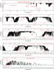 |
Fig. 1 Synthetic absorption spectrum of the sky between 0.3 and 30 μm calculated with LBLRTM (resolution R ~ 10 000) using the annual mean profile for Cerro Paranal (Noll et al. 2012). The eight main molecules O2, O3, H2O, CO, CO2, CH4, OCS, and N2O contribute more than 5% to the absorption in some wavelength regimes. The red regions mark the ranges where they mainly affect the transmission, minor contributions of these molecules are not shown. The green regions denote minor contributions (see Table 1) from the following molecules: (1) NO; (2) HNO3; (3) COF2; (4) H2O2; (5) HCN; (6) NH3; (7) NO2; (8) N2; (9) C2H2; (10) C2H6; and (11) SO2. |
Species with a minor line-absorption contribution.
3. Description of the molecfit telluric correction tool
The molecfit package allows one to simulate and fit tropospheric and stratospheric emission or absorption telluric lines affecting user-selected region(s) of an observed (usually, science) spectrum. It uses parameters provided in a configuration file and, if present, the FITS header of the spectrum. It then returns a transmission spectrum for the whole wavelength range of the spectrum.
Molecfit includes the following ingredients:
-
1.
an automatic retrieval of two atmospheric profiles from theGlobal Data Assimilation System (GDAS) web site. Theseprofiles bracket the time of the observation and can be retrieved forany observatory in the world. These profiles are linearlyinterpolated to match the time of the observations and mergedwith a standard profile and local meteorological data to create aninput profile for the radiative transfer code;
-
2.
a radiative transfer code that simulates atmospheric emission and transmission spectra;
-
3.
a molecular spectroscopic database;
-
4.
a simple grey-body calculator that simulates the contribution of the continuum from the instrument and telescope;
-
5.
a choice of possible line spread functions (also referred to as kernels);
-
6.
an automatised fitting algorithm that adjusts the continuum spectrum, wavelength calibration, spectral resolution, and column density of each of the relevant molecules, with the possibility of excluding spectral regions expressed either in pixels or in wavelength regions.
In the following, we describe important aspects of these components in more detail. We also discuss specific choices made for the ESO Paranal observatory.
3.1. Atmospheric profile
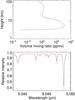 |
Fig. 2 Top: two examples of the distribution of the water-vapour volume-mixing ratio as a function of altitude. The black solid line corresponds to a volume-mixing ratio of 0 ppmv up to 3.1 km (Paranal altitude is 2.6 km), while the red dashed line corresponds to a constant relative humidity until 3.1 km. The total amount of precipitable water vapour, 2 mm, is identical for both profiles. Bottom: sample of the corresponding transmission spectra at R = 100 000. The higher amount of water vapour in the lower atmospheric layers above the observatory leads to both deeper cores and stronger continuum absorption. |
An atmospheric profile typically describes the temperature T, pressure P, and volume mixing ratio x of several molecular species as a function of altitude h for a given location. These parameters have a direct impact on the shape and strength of all the telluric lines. For molecfit we use a merged profile based on a reference atmospheric profile, modelled 3D data, and on-site meteorological measurements.
The reference atmosphere profile is by default the equatorial profile derived by Remedios7. It contains abundances of several molecular species up to an altitude of 120 km, divided into 121 altitude levels. Owing to the low latitude of Cerro Paranal (Lat: –24.6°), the equatorial profile is better suited (Anu Dudhia, priv. comm.) than the tropical or standard profiles, which are also available in the molecfit package. We note here that the molecular composition has changed since the profile was created in 2001. In particular, the content of the greenhouse-gas carbon-dioxide content has increased by ~6% (World Meteorological Organization 2012). Molecfit allows the user to either fit or manually adjust the molecular content to take this increase into account. Alternatively, the reference atmosphere used by molecfit can be easily modified to another existing or manually created profile.
The reference atmosphere is then merged with the modelled GDAS8 3D data provided by the National Oceanic and Atmospheric Administration9 (NOAA). This model contains time-dependent information on the temperature, pressure, relative humidity, wind speed, and direction up to an altitude of ~26 km on a 3 h basis. Owing to the geographical 1° × 1° grid, we created a set of profiles by means of an interpolation of the four grid points closest to Cerro Paranal to obtain local information. The GDAS profile derived for a specific observation is then by default a linear interpolation of the two resulting profiles closest in time to the observation. The molecfit package contains all the available GDAS profiles for Cerro Paranal since December 1, 2004 at 00:00 UT and the release date of the package. In addition, ESO will regularly maintain such a database for Paranal. For observations obtained later or from another site, molecfit automatically retrieves the appropriate GDAS files.
It may still be possible that no GDAS profiles are available for the time of observations. In the case of Cerro Paranal, molecfit then use the best matching two-month average (Noll et al. 2012). Alternatively, an ASCII profile with the same format as a GDAS profile can also be provided by the user.
A further optional refinement of the final profile is achieved by incorporating on-site measurements obtained by the Astronomical Site Monitor (ASM) as provided in the FITS header or through a parameter file. The influence of the measured values at the observatory altitude is gradually decreased up to a configurable upper mixing height, set by default to ~ 5 km, where, for Paranal, the wind direction changes by an average of ~ 90° on average, as revealed by an analysis of the GDAS wind data. Thus, it can be assumed that at this altitude the influence of the local environment (as determined from the ASM data) has diminished. More information on the merging procedure can be found in the UM.
Water vapour is the molecule showing the most variations because its total amount (PWV) and its altitude distribution can change significantly and on a short time scale. In particular, the largest amount of PWV may not be located in the lowest layers of the atmosphere. Figure 2 illustrates the importance of having a decent profile for water vapour.
The total amount of PWV can optionally be set if the value can be retrieved independently (for example, from radiometer measurements, see Kerber et al. 2012). In this case, the merged profile composed by the reference atmosphere, the GDAS data, and the local meteo information will be scaled to the requested PWV. Alternatively, the atmospheric profile provided by the radiometer – soon retrievable from the ESO archive – can be used directly.
 |
Fig. 3 Effect of ground temperature or pressure variation on the H2O telluric spectrum for two different spectral ranges. Each graph shows the ratio between telluric spectra computed with the indicated ground temperature or pressure. Top:variation of 1 °C and 10 °C. The region close to 3.68 μm shows opposite behaviours. Bottom: variation of 1 mb and 10 mb. |
Figures 3 illustrates the effect of the variation of the ground temperature and pressure on the H2O telluric spectrum. Depending on line parameters, different lines behave differently with temperature or pressure.
3.2. Radiative transfer code
The resulting merged atmospheric profile is used as input in the radiative transfer code LNFL/LBLRTM (Clough et al. 2005). The version used at the time of the first release of the molecfit package is the latest version at that time, V12.2. This code package is widely used in atmospheric sciences and is publicly available. It calculates radiance and transmission spectra with a spectral resolving power of about four million. More information can be found at the web site10.
3.3. Database of molecular parameters
In addition to the profile, the radiative transfer code requires a line database as input. The first release of molecfit uses the database aer_v_3.2, which is delivered with the LNFL/LBLRTM code package: it is based on an updated version of the HITRAN 2008 database (Rothman et al. 2009) and contains information on more than 2.7 million spectral lines of 42 molecular species (see Table 2). Themolecfit line database can be easily updated when a new version becomes available.
Only molecules for which an atmospheric volume mixing ratio is available in the standard atmosphere profile provided with molecfit can be used by default. These molecules are identified in Table 2.
List of molecules as provided by the aer line parameter database.
3.4. Fitting algorithm
Molecfit makes use of the C version of the least-squares fitting library MPFIT (Markwardt 2009) based on the FORTRAN fitting routine MINPACK-1 (Moré 1978). It uses the Levenberg-Marquardt technique to solve the least-squares problem leading to a fast convergence even for the complicated functions involved in molecfit, while being numerically robust and self-contained and allowing upper and lower limits or parameters tied to each other that can be individually set.
3.5. Inclusion and exclusion regions
A spectrum shows a number of features that can be characterised in the following way:
-
intrinsic features from the science object,
-
telluric features,
-
intrinsic features from the instrument caused either by the spectrograph or the detector.
Intrinsic features either from the science object or from the instrument can interfere with the fitting process.
Therefore, molecfit allows one to:
-
select inclusion regions, also called fitting ranges, whose mainpurposes are to allow molecfit to determine the column densityof the relevant molecules and the line spread function (or kernel).Such regions must therefore show a good enough continuumlevel for the fitting accuracy and include telluric absorption linesfor determining the line spread function. One or several suchregions must be defined so that at least some telluric lines fromeach molecule to be corrected are covered;
-
select exclusion regions within the inclusion regions that are affected by the presence of intrinsic features from the science objects;
-
mask pixels in the inclusion regions that are affected purely by instrumental or detector effects.
Details can be found in the UM.
3.6. Continuum contribution
The model spectrum, Fout, is scaled by a polynomial of degree nc: 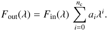 (1)For a0 = 1 and all other ai = 0, the model spectrum remains unchanged. This is the default configuration for the initial coefficients. The continuum correction is carried out independently for each fitting range. A fitting range (or the full spectrum) is split further if it is distributed over more than one chip.
If the input spectrum is an emission line spectrum, an optional flux conversion can be carried out in order to match the unit of the synthetic spectrum. Further details are available in the UM.
3.7. Telescope background
For sky emission modelling, the telescope background is assumed to be a grey body (black body times emissivity). The parameters of this grey body correspond to the telescope main mirror temperature and an effective emissivity of the telescope and instrument.
3.8. Wavelength calibration
The science spectra to analyse are expected to have an accurate wavelength calibration. However, small errors can affect the determination of the line spread function and column densities negatively. Therefore in each inclusion region, the synthetic spectrum being fitted can be adjusted to match the input spectrum. A Chebyshev polynomial of degree nw is used for this purpose: 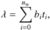 (2)where
  (3)where the wavelength range is normalised so that λ′ ranges from −1 to 1 over the entire spectral range of the spectrum or, in the case of multi-chip instruments, over the range covered by an individual chip.
The conversion of the wavelength grid to a fixed interval results in coefficients bi independent of the wavelength range and step size of the input spectrum. For b1 = 1 and all other bi = 0, the model spectrum remains unchanged. This is the default configuration for the initial coefficients.
On the other hand, in some cases, one wishes to use the telluric lines as references to improve an unsatisfactory initial wavelength calibration. This is the case for CRIRES in particular. For such a purpose, molecfit actually outputs the inverse of the wavelength calibration described in Eq. (2), in the sense that the input spectrum is then adjusted to match the synthetic one. Such wavelength calibration is only meaningful when the inclusion range covers the whole spectrum and is sampled well by telluric lines.
3.9. Line spread function
The model spectrum is convolved with up to three different profiles to determine the shape of the line spread function. They are:
-
1.
a simple boxcar
 (4)which is adapted to the pixel scale and normalised to an integral of 1. This kernel is particularly useful for objects fully covering the entrance slit; and
 -
2.
a Gaussian
 (5)centred on 0, where
 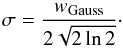 (6)The full width at half maximum (FWHM), wGauss, is given in pixels.
 -
3.
A Lorentzian
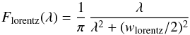 (7)centred on 0, where wlorentz is the FWHM in pixels. Compared to a Gaussian, the Lorentzian approaches the 0-level flux significantly more slowly.
A kernel consisting of all three components is usually too complex to be constrained by a fit. To avoid unrealistic best-fit FWHM, the user should reduce the number of degrees of freedom by fixing individual fit components. A FWHM of zero pixel corresponds to a unity convolution; in other words, it does not change the input spectrum.
Alternatively, the user has the possibility of choosing a single Voigt profile kernel directly, which is then calculated by an approximate formula that takes the FWHM of Gaussian and Lorentzian as inputs. The user can also select a kernel whose size in pixels linearly increases with wavelength. It is suitable for an instrumental setup with nearly constant resolving power, fixed wavelength step size, and a wide wavelength range, such as cross-dispersed echelle spectrographs.
Finally, a user-defined kernel can be provided in the form of an ASCII table of fixed kernel elements. This option overrules the parameterised kernel discussed above. An inappropriate kernel can cause deviations in the determination of molecular column densities of more than 10%.
3.10. Molecular volume-mixing ratio
The integrated volume mixing ratio, X(h0), of a molecule for a column of air from the observer at an altitude h0 to the top of atmosphere can be derived by 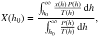 (8)if the mixing ratio (or mole fraction) x, air pressure P, and temperature T are given depending on altitude h by an atmospheric profile. Volume-mixing ratios are usually given in part per million in volume (ppmv).
For H2O, it is also common to provide the column height of PWV in mm (also referred to as amount of PWV). It can be calculated by 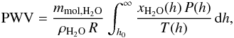 (9)where the mole mass of water mmol, H2O = 0.0182 kg, the density of liquid water ρH2O ≈ 103 kg m-3, and the gas constant R = 8.31446 J mol-1 K-1. The required units of x, P, T, and h are ppmv, Pa, K, and km, respectively. Molecfit outputs the column height for other gases using a similar formula.
Since the GDAS profiles and the ESO MeteoMonitor data provide an H2O volume-mixing ratio as relative humidity RH in percent, it has to be converted to x. For this purpose, we have implemented the approximations for vapour pressures of ice and supercooled water as function of temperature as described by Murphy & Koop (2005). The minimum of both then corresponds to the saturated vapour pressure Psat, which is used to estimate the altitude-dependent x in ppmv by 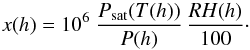 (10)Molecfit allows the user to adjust this quantity based on the observed telluric lines, and we note that the GUI only allows one to fit the column density for the molecules indicated in the last column of Table 2. This adjustment is done by multiplying the overall atmospheric profile by a single constant. For most molecules, the impact is actually limited to the lowest atmospheric layers.
3.11. Supported instruments
One-dimensional (1D) spectra of any visible, near-, or mid-infrared instrument could in principle be used by molecfit. Details on the required information can be obtained in the User Manual (Noll et al. 2013). Although the tool has been tailored to ESO-Paranal instruments – in particular, the GDAS profiles are available as a tarball file only for this site – there are no specific limitations either in the terms of format or in geographical location for a ground-based observatory.
3.12. Inputs and outputs
Molecfit accepts 1D spectra provided as ASCII tables, FITS tables, and images. The FITS tables can have several extensions corresponding to different chips (e.g., CRIRES). Required keywords are either taken from the FITS header or directly from the parameter file. Finally, ASCII or FITS files for inclusion and exclusion regions can be provided.
Molecfit fits the synthetic spectrum in the inclusion regions alone. These regions can cover just a small fraction of the wavelength range or all of it. It returns the best-fit model only for the inclusion regions in both an ASCII and a FITS table, and the best-fit parameters and molecular column densities (including the PWV) in a results ASCII file.
The molecfit package then outputs a transmission spectrum and the division of the input spectrum by the transmission spectrum over the full spectral range of the input spectrum. Apart from results tables in ASCII and FITS format, the corrected spectrum is written into a file in the same format as the input spectrum (see the UM for more details).
In addition, molecfit can provide a new wavelength calibration based on the telluric lines as described in Sect. 3.8. This two-step approach greatly improves the speed of the overall process.
3.13. Expert mode
In most cases molecfit is able to determine the different user-selected parameters automatically with a minimum of configuration. However, in a few cases, mostly for CRIRES, a much greater flexibility is needed. An expert mode is therefore also provided. It allows the user to fit the spectra on each inclusion range individually and provides him/her the access to the coefficients of the polynomials for the continuum and wavelength correction. Moreover, the parameter file with the best-fit values for all parameters is saved and can be used for another iteration of molecfit.
3.14. Fitting sky emission spectra
The tool is able to fit sky emission spectra for molecules and physical processes handled by the radiative transfer code, with the exclusion of lines produced by chemiluminescence (such as OH, see, e.g., Noll et al. 2012). In other words molecfit can in principle determine the line spread function and column densities of the relevant molecules and therefore derive the transmission spectrum of the atmosphere based the sky emission spectrum if the spectral range is located in the thermal infrared.
4. Impact on observing strategy
Although powerful, molecfit is not necessarily suited to telluric corrections in all cases. In this section, we briefly discuss a few situations to consider while deciding on the details of the observing strategy for the absorption telluric correction.
4.1. Main cases
Two main cases for the use of molecfit can be considered, depending on whether the wavelength calibration of the spectrum is reliable and accurate (root-mean-squared residuals ≈0.1 pixel or better) or not.
In the case of accurate wavelength calibration, the main requirement is that the spectrum to be corrected has at least one spectral region that includes medium-strength molecular lines of the most variable relevant species and that these lines are isolated enough so that their column density and the line spread function can be determined.
If the wavelength calibration is not reliable but needs to be corrected by molecfit based on the telluric lines themselves, a – possibly delicate – selection of inclusion and exclusion regions must be carried out, such that only telluric lines appear in the inclusion regions and that any intrinsic feature of the object is masked out in the exclusion regions. In case the continuum needs to be refined by molecfit, the fitting regions need to present enough coverage to be able to determine either an overall continuum or local continua.
4.2. Simple continuum shape and small number of intrinsic features
The easiest spectra that can be modelled by the tool are the ones for objects with a well-defined and simple continuum and with limited confusion between telluric and intrinsic features. In such conditions, the tool can properly model the continuum spectrum of the object, and the parameters of the telluric features can be well constrained.
4.3. Large number of intrinsic features
If the number of intrinsic features is large in the spectral domain of interest, several options are possible. The choice of the best option depends on the line crowding: a first constraint is the number of points that can be used to determine the spectral continuum; a second constraint is the number of spectral ranges where telluric lines can be used to determine the column density of the molecules contributing in this spectral domain. An additional constraint arises if the wavelength calibration is not reliable.
Therefore a possible strategy is first to observe a telluric star with the same setup – or retrieve corresponding data from the archive – and use molecfit on its reduced spectrum to determine which molecules are relevant, the wavelength calibration or continuum level. Then, molecfit can be applied to the science target using the derived wavelength calibration (if relevant), changing the airmass, or fitting the continuum and/or the column densities of the molecules involved. An example of such a strategy is shown below in Sect. 6.8 and is illustrated in particular in Fig. 12. Another possible strategy is to ensure that the spectral setup includes spectral regions containing representative telluric lines but free of intrinsic lines.
4.4. Emission line spectra
The telluric transmission spectrum cannot be fitted on the spectrum of an object showing little or no continuum, such as a faint cometary spectrum or an emission line object. A suggested strategy in this case is either to retrieve a spectrum of a telluric star from the archive or observe a telluric star in the spectral set-up of interest. Its spectrum can be modelled by molecfit. The model can then be modified easily by changing the airmass such that it corresponds to the airmass of the science target. If the water vapour at the site is monitored, the model can also be modified accordingly. The number of times telluric stars need to be observed is therefore reduced significantly.
5. Limitations
In this section, we briefly discuss the various factors that limit the accuracy of the molecfit correction of telluric spectra. Such factors can be external to molecfit, and are related to the accuracy with which instrumental parameters are taken into account or are internal to the method itself.
5.1. External
Molecular parameters’ accuracy and completeness:
a first limitation arises owing to the completeness of the incorporated line database and on the accuracy of the contained molecular parameters. Currently, the AER line database delivered with the LBLRTM code is included by default with molecfit. It is usually more frequently updated than the underlying main HITRAN11 and is therefore recommended. However, although molecfit a priori allows one to use the original HITRAN database, this functionality is subject to the stability of the database structure.
Molecules in atmospheric profile:
Molecfit only offers the possibility to fit the overall volume mixing ratio along the line of sight in the atmosphere: the overall shape of the profile is not adjusted. If the actual profile differs from the modelled one in some atmospheric layers, systematic errors can occur. In particular such a situation can be caused by the specific, temporary volume-mixing ratios of a molecule and is relatively frequent for water vapour. Figure 2 illustrates the possible impact in an extreme case.
In particular, the accuracy of the transmission spectrum derived from sky emission as described in Sect. 3.14 strongly depends on the precision with which the retrieved atmospheric profile actually represents the true one.
Atmospheric profile stability:
any correction of telluric absorption requires a relatively stable atmosphere. The arrival of an atmospheric front is a clear case where the atmospheric profile changes suddenly. Even if the GDAS profiles would show such a front, its precise timing and characteristics are usually uncertain and surely depend on the pointing direction. Fortunately, few optical or infrared astronomical observations are executed in such conditions.
Radiative transfer code accuracy:
the reader is referred to the publication list available on the LBLRTM web page12 for references regarding the validation of the radiative transfer code. In particular, it is worth repeating here that “the algorithmic accuracy of LBLRTM is approximately 0.5% and the errors associated with the computational procedures are of the order of five times less than those associated with the line parameters so that the limiting error is that attributable to the line parameters and the line shape”.
5.2. Instrumental
Grating scattering:
internal diffusion strongly limits the achievable accuracy of the modelling. Villanueva et al. (priv. comm.) found that the CRIRES line spread function is best reproduced by a Voigt profile that needs to be calculated over ≈1000 pixels to account for the grating scattered light within the instrument. As a consequence, it often appears that the core of heavily saturated absorption lines does not reach zero intensity. The amount of flux in the core actually depends on the spectral energy distribution of the light reaching the grating and cannot be modelled accurately by molecfit, because molecfit only applies the convolution of the line spread function to the transmission spectrum and not to the science target one. In addition, later investigation (Uttenthaler 2010, priv. comm.) indicates that the spatial profile of the grating scattered light is different from the one of the direct light.
The observed spectrum therefore combines different effects that cannot be easily modelled by molecfit. Therefore they limit the accuracy of the correction such that residuals can reach an estimated 1% of the continuum depending on the significance of the grating scattering.
Instrumental background:
when modelling sky emission spectra, molecfit uses a background defined by a grey body at the temperature of the main mirror of the telescope. It assumes that the thermal background from the instrument is negligible.
Instrumental response curve shape:
Molecfit fits a low-order polynomial to the observed continuum of the input (object spectrum) for each inclusion region. However, it does not make a difference between the intrinsic continuum shape and the effect of the response curve of the instrument. Good results are obtained if the observed continuum of each inclusion region can be modelled well by such polynomials. Alternatively, the user may provide a normalised spectrum as input.
Line spread function:
the line spread function should behave well over the wavelength range of interest, either being constant or having a width that is linearly dependent on wavelength, as expected in cross-dispersed spectrographs.
When the transmission spectrum is derived from the sky emission spectrum (Sect. 3.14), one should note that the parameters of the line spread function are likely to be different from the one of the science target given that the image of the star does not uniformly illuminate the entrance slit.
5.3. Internal
Good internal guess values:
by essence of the Levenberg-Marquardt fitting approach, molecfit needs and is sensitive to the initial guess solution. In particular, molecfit is designed to refine the wavelength calibration and continuum determination, but it is not designed to measure these values from an uncalibrated spectrum. Adequate initial estimates improve the robustness of the fit and the speed of the convergence process. Knowledge of the line spread function and spectral resolving power are also important, although the latter can be adjusted by molecfit.
Finite pixel size:
Molecfit results are best when the spectral resolution is at least Nyquist sampled by the instrument. In any case, molecfit takes the finite pixel size of the spectrum into account: molecfit estimates the highest pixel resolution in a spectrum by evaluating the wavelength grid. An oversampling factor of 5 is then applied on the input to the radiative transfer code.
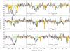 |
Fig. 4 H2O telluric absorption lines affecting absorption lines associated with the z = 2.42743 DLA in the UVES spectrum of GRB080310. The telluric lines – modelled by molecfit – are shaded in yellow; the models for the different components (a,b,c,d) of the absorption system are represented with different colours (blue, cyan, green, orange), while the combined model is in red. See De Cia et al. (2012) for details. |
6. Examples
In the following, we illustrate the versatility of molecfit through its application to data sets obtained with various ESO VLT instruments covering a range of spectral resolving powers and wavelength domains.
6.1. UVES
The prototype version of molecfit was manually adjusted to determine the location and strength of telluric absorption lines in VLT UV-Visual Échelle Spectrograph (UVES, Dekker et al. 2000) rapid response mode or target-of-opportunity programmes of γ-ray bursts (UVES is a high-resolution cross-dispersed spectrograph in the visible): indeed, some H2O lines mimic lines associated with high-redshift damped Ly-α (DLA) lines. For example, in the spectrum of GRB050730 (Ledoux et al. 2009) obtained under Programme ID 075.A-0603 (P.I.: Fiore), H2O lines appear coincident in wavelength with the Si ii  λ1816 line, and affect the Fe ii
  λ1267 and Fe ii
  λ1659 lines, all associated with the z = 3.69857 DLA. Similarly, as shown in Fig. 4, using molecfit allowed the location and strength of the H2O lines affecting the Fe ii λ2382, λ2374, Fe ii
  , and λ2389 lines to be determined (amongst others) associated with the z = 2.42743 DLA in the spectrum of GRB080310 (De Cia et al. 2012) obtained under programme ID 080.D-0526 (P.I.: Vreeswijk).
6.2. FLAMES
Figure 5 presents a Fibre Large Array Multi Element Spectrograph (FLAMES)/Giraffe spectrum of the O4 V star NGC 3603-117 observed with the LR8 setting and the ARGUS integral field unit (data courtesy of M. Gieles; Prog. ID: 079.D-0374(A)), providing a spectral resolving power of R ≈ 10 400. The presented spectrum corresponds to the brightest spaxel on the object.
The presence of water-vapour telluric absorption lines impedes any precise determination of the width and centroid of the Paschen hydrogen lines at 901 and 923 nm. However, there is usually no observation of telluric stars for FLAMES. Molecfit can be used to determine the PWV and to correct the science spectrum by the transmission spectrum. As a result, a precise determination of the width and position of the lines can be obtained by multiplying the number of stellar lines available by three for, e.g., radial velocity measurements in that spectral region.
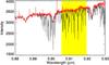 |
Fig. 5 FLAMES/Giraffe Spectrum of NGC 3603-117. Black: original spectrum. Red: telluric line corrected spectrum. The spectral range covered by the shaded area was used to determine the amount of PWV. |
6.3. SINFONI
Archival data of the field of the binary star 2MASS J01033563-5515561 obtained with the Spectrograph for INtegral Field Observations in the Near Infrared (SINFONI, Eisenhauer et al. 2003) for programme ID 290.C-5022(A) (P.I.: Delorme) were retrieved and reduced with the SINFONI pipeline and default parameters. Only 20 s Detector Integration Time (DIT) J-band exposures obtained at a median airmass of 1.28 are shown here. The telluric star Hip 024337 was observed at an airmass of 1.33, approximately 66 min after the start of the first science exposure. The spectra of the secondary star (B) and of the telluric star were extracted using a three-pixel radius centred on the photo-centre of each source. Hot pixels or cosmics in the reduced spectrum affected were manually edited out.
Inclusion regions were selected to cover telluric lines caused by H2O and O2. Exclusion regions were defined for the pixels affected by cosmics. Figure 6 shows the original spectrum and compares its correction by the transmission spectrum calculated by molecfit and by the telluric star. The spectrum corrected by the transmission spectrum calculated by molecfit is slightly less noisy than the one corrected by the telluric star spectrum, and it does not show the effect of the H i Paschen β line. On the other hand, the correction of the lines in the ~ 1.13 μm water vapour band is slightly less good probably because of a small change in the line spread function.
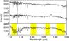 |
Fig. 6 SINFONI J band spectrum of 2MASS J01033563-5515561 B. Bottom: pipeline reduced spectrum. The yellow shaded areas show the spectral ranges of the inclusion regions. Exclusion regions appear in blue. Medium: spectrum divided by the spectrum of the telluric star. Top: spectrum divided by the transmission spectrum calculated by molecfit. |
6.4. X-shooter
A reduced X-shooter (Vernet et al. 2011) spectrum of the luminous blue variable star R71 was kindly provided to us by Andrea Mehner. X-shooter is an instrument composed of a UV, a visible, and a near-infrared cross-dispersed medium-resolution spectrograph. The data were obtained on February 1, 2014 as part of the programme ID 092.D-0024(A) (P.I.: Baade). The slit width used was 5″ × 11″ and the exposure time 20 s. Figure 7 shows the visible part of the original spectrum together with the spectrum corrected by the transmission spectrum calculated by molecfit, based on the fitting made in the regions marked in in the shaded regions.
The wide slit used means that the line spread function is dominated by the image quality at the time of the observations (FWHM ≈ 2′′ in this case) and not by the slit width. No telluric star was observed with the same instrumental setup because the observation was obtained to correct the flux loss suffered by spectra obtained later with a narrow slit. Even if a telluric star had been obtained, its usefulness for telluric line correction would have strongly depended on the stability of the seeing.
Given the overheads associated with such a short integration time, the time spent executing the observation of the telluric star would have been roughly 100% of the time spent executing the observation of the science target: therefore, molecfit also allows one to correct telluric features in spectra obtained with a slit larger than the image quality.
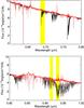 |
Fig. 7 Visible arm X-shooter spectrum of R71 LBV star. The pipeline reduced spectrum is shown in black. The shaded areas show the inclusion regions used to model the line spread function and determine the column densities of H2O and O2. The spectrum corrected by the derived transmission spectrum is shown in red. |
6.5. VISIR
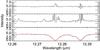 |
Fig. 8 VISIR high-resolution λ12.279 μm spectrum of HD 1043 27. Bottom: pipeline reduced spectrum. In red, the result of the fit obtained with molecfit. Medium: spectrum divided by the telluric star. Top: spectrum divided by the transmission spectrum calculated by molecfit. |
Archival data of HD 104 237 obtained with the VLT Imager and Spectrometer for mid InfraRed (VISIR) for programme 076.C-0129 (P.I.: van den Ancker) were retrieved and reduced with the VISIR pipeline v. 3.5.1 and default parameters. Only the 12.279 μm HRG spectrum is shown here. The airmass ranged from 1.68 to 1.72.
A first attempt to use molecfit on the spectrum of HD 104 237 did not provide a good correction. Analysis of the residuals showed the presence of low frequency variations of the response curve, on a scale similar to the size of the telluric lines, and therefore difficult to correct by the continuum fitting implemented within molecfit. Indeed, the VISIR calibration plan does not include any flat fields that could correct an effect normally taken care of by the observation of telluric standards. To alleviate this problem, molecfit was used on the associated telluric star HD 92 305, which actually shows photospheric absorption lines. The same low-frequency variations can be seen in the spectrum of the telluric star divided by the molecfit model, which was then fitted by a seventh-degree polynomial. This continuum model was then applied to the reduced spectrum of HD 104 237 before another attempt with molecfit. This time the fit is very satisfactory, as can be seen in Fig. 8, which can be compared with the one for the same object shown in Fig. 1 of Carmona et al. (2008).
Molecfit offers the advantage of (a) less telescope time used for observation of a telluric star: in this case, the execution of the observation for the telluric star took 36 min compared to the two hours used for the science target; (b) the telluric star was observed with an airmass difference of about 0.1, which is sufficient to lead to significant differences in the wings of the telluric lines where the molecular H2 0–0 S(2) (J =4–2) emission at 12.278 μm emission line was expected; (c) the telluric star shows photospheric lines that must be properly identified and corrected for.
6.6. KMOS
Reduced spectra (incl. sky subtraction) of three red supergiant stars of Barnard’s galaxy NGC 6822 simultaneously obtained during the K-band Multi Object Spectrograph (KMOS, Sharples et al. 2013) science verification programme 60.A-9452 (P.I.: C. Evans) were kindly provided to us by Lee Patrick (Patrick et al., in prep.). KMOS deploys 24 arms to user-selected 2.8″ × 2.8″ areas at a spatial sampling of 0.2″ × 0.2″ in a 7.2′ diameter field feeding 24 integral-field units sending light to three near-infrared medium-resolution spectrographs. The three stars were chosen such that their spectra were obtained on different spectrographs. The YJ filter/grating setup was used. See Table 3 for the correspondence between star IDs, coordinates, arms, and spectrographs. For the purpose of this paper, the determination of the column densities for the relevant molecules was done using only the spectrum of star #8, and the determined values were then used as constant for the two other stars. On the other hand, the parameters of the line spread function were determined independently on each spectrum.
The execution time required for the spectra shown in Fig. 9 is slightly more than 1h. Observation of the same telluric star (HD 187 439 of spectral type B6III) for each arm was carried out right after and took 15 min, i.e. ≈25% of the time devoted to the science. The telluric stars were chosen by the user, but the difference in airmass between the science target (ranging from 1.45 to 1.98) and telluric star (ranging from 2.00 to 2.13) observations make the corrections by the telluric star challenging. Instead, molecfit here again allows one to avoid such problems.
Therefore in a number of cases molecfit produce very satisfactory telluric corrections for KMOS. It would be interesting to determine if the line spread function can be modelled well enough as a function of rotation angle and temperature to avoid the need for systematic observations of telluric stars. Such a study is outside the scope of this paper.
6.7. MUSE
Correspondence between star ID, coordinates, KMOS arms, and spectrographs.
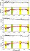 |
Fig. 9 KMOS spectra of 3 red supergiant stars in NGC 6822, each feeding a different spectrograph. From top to bottom: star #40, star #36, and star #8. In each figure, the bottom graph shows the reduced data in black, while the spectra corrected by the synthetic spectrum determined by molecfit is shown in red; the top graph shows the star spectrum corrected by the telluric star observed just after. The molecular column densities were determined using only the spectrum of star #8: the results were used on the spectra of stars #36 and #40. The line spread functions were, however, determined on each spectrum independently. The yellow shaded areas indicate the inclusion regions, while the blue shaded areas show the regions excluded from the fit because they correspond to spectral features intrinsic to the stars. |
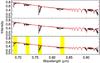 |
Fig. 10 MUSE spectra of 3 stars in the globular cluster NGC 6 397. The reduced data appear in black, while the spectra corrected by the synthetic spectrum determined by molecfit are shown in red. The molecular column densities and line spread function were determined using only star #5326 (bottom) located on IFU #7: the results were used on the spectra of star #10327, also located on IFU #7 (middle), and #10893 (top), located on IFU #13. The yellow shaded areas indicate the inclusion regions. No regions were excluded from the fit. |
Correspondance between star ID, coordinates, and MUSE IFUs.
Reduced spectra of three stars of the globular cluster NGC 6 397 obtained during the Multi-Unit Spectroscopic Explorer (MUSE) (Bacon et al. 2010) commissioning 2B (programme ID: 60.A-9100(C)) were kindly provided to us by Roland Bacon and Sebastian Kamann. MUSE is an integral field spectrograph composed of 24 identical IFU modules sampling a 1′ × 1′ field-of-view at (0.2″ × 0.2″) spatial resolution and up to R ~ 3000 spectral resolving power. The three stars were chosen such that their signal-to-noise ratio is greater than 100 and so that two of them fall on the same IFU and the third one on a different IFU. See Table 4 for the correspondance between star ID, coordinate, and IFU. The column densities for the relevant molecules (O2, H2O) and line spread function were determined using only the spectrum of star #5326. The derived transmission spectrum was then applied to the other stars, #10327 and #10893.
The very good wavelength calibration and the similarity of the line spread functions between IFUs explain that the same transmission spectrum can be used for these IFUs. Molecfit can therefore potentially be used to correct for telluric absorption for all 90 000 spectra obtained by MUSE at once, provided a suitable star falls in the field of view. The spectral resolution of the instrument seems low enough not to be affected by the details of the atmospheric profiles described in Sect. 3.1, so that molecfit can be used on a spectrum resulting from the combination of multiple observations spread over several, but not necessarily successive nights.
6.8. CRIRES
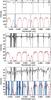 |
Fig. 11 Extract (detector #2) of CRIRES 4889.5 nm setting spectra of γ Gem(top), α For(middle), and Barnard’s star(bottom). In each case, the bottom graph shows the original, reduced spectrum and the blue-shaded exclusion regions; the red spectrum shows the molecfit derived transmission spectrum scaled by a constant factor. The top graph shows the molecfit corrected spectrum. |
 |
Fig. 12 Extract (detector #2) of CRIRES 4889.5 nm setting spectra of X TrA; the red spectrum shows the molecfit-derived transmission spectrum scaled by a constant factor. The top graph shows the corrected spectrum. Molecfit was used in expert mode in this case. |
Spectra obtained with the Cryogenic high-resolution IR Échelle Spectrograph (CRIRES, Käufl et al. 2004) before mid-July 2014 – when the instrument was removed from operations to undergo an upgrade – covered a narrow spectral range (Δλ ≈ λ/ 70) at a resolution R ~ 50 000 to 100 000. Although the line spread function is usually well modelled by a Gaussian function (Seifahrt et al. 2010), its wings are more Lorentzian. Therefore a Voigt profile is usually best for representing it (Villanueva et al., priv. comm.), in particular, to attempt to model the light scattered on the grating that causes even heavily saturated lines to appear with residual light in their core. The kernel width, on the other hand, depends on the quality of the adaptive optics (AO) correction – when the AO is used – which in turn depends on the “AO star” magnitude and on the turbulence profile of the atmosphere. On the other hand, for non-AO observations, it may also depend on the actual slit width; one should note here that the slit mechanism lacked reliability before the installation of fixed slit widths in September 2011 (Smoker 2014).
As mentioned in the CRIRES User Manual (Smoker 2014), CRIRES spectra are often affected by imprecise wavelength calibration, owing to a lack of calibration lines. Molecfit can solve this problem in a number of situations using the telluric lines themselves when they are distributed well over the spectral range and not too mixed with lines that are intrinsic to the science target.
Figure 11 shows an extract (detector #2 only) of the 4889.5 nm setting spectra for three stars obtained as part of the CRIRES-POP programme (Lebzelter et al. 2012): the A0 IV star γ Gem, observed on October 20, 2010 (programme ID 086.D-0066, P.I.: Lebzelter); the F8 V star α For, observed on October 31, 2009 (programme ID 084.D-0912, P.I.: Lebzelter); and the M4 V Barnard’s star, observed on July 7, 2010 (programme ID 086.D-0066, P.I.: Lebzelter). No telluric stars were observed for this programme. The number of intrinsic lines increases for late-type stars, thus requiring an increase in the number and size of exclusion regions; consequently, an F8V star is approximately the latest star for which molecfit can be used in a non-expert mode.
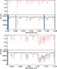 |
Fig. 13 Extract (detector #3) of CRIRES 2332.2(top) and 2368.7 nm (bottom) setting spectra of Procyon. In each figure the top graphs show generic (not model) transmission spectra for the relevant molecules: H2O in black, CH4 in red, CO2 in green. The bottom graphs show the original pipeline reduced spectra in black, as well as the molecfit-corrected spectra, in red. The dotted lines show 2% deviation from the median value of the corrected spectra. |
Representative measurements of the accuracy of the telluric correction in spectral ranges affected by unsaturated or moderately saturated lines.
For later stars, the expert mode (see Sect. 3.13) is required. The variable carbon star X TrA was observed on September 22, 2010 as part of the same programme. Regarding the molecular content of the atmosphere, molecfit was configured to fit only the column density for H2O and CO2, while the O3 and OCS column densities were fixed. The polynomial coefficients for the continuum and wavelength calibration were copied from the results of the fit to the γ Gem spectrum. The wavelength solution found for γ Gem was kept fixed. This method allowed one to obtain very good results for the telluric line correction, as shown in Fig. 12.
To illustrate the quality of the correction on high signal-to-noise spectra, we used molecfit on the 2332.2 and 2368.7 nm setting spectra of the F5 IV star Procyon observed on November 7, 2011 (programme ID 088.D-0109, P.I.: Lebzelter). The signal-to-noise ratios – estimated on clean regions of the molecfit-corrected spectra – are ~350 and 400, respectively. Figure 13 clearly indicates a very good correction, well within 2% except for the core of the moderately saturated lines. A slight difference in the quality of the correction can also be seen between H2O and CH4 lines, most likely caused by slight errors in the atmospheric profiles.
Observations of telluric stars with CRIRES can easily take longer than for the science targets. Given the high signal-to-noise of the spectra obtained, differences in observing conditions and in airmass may significantly affect spectra corrected by telluric standards. The use of a tool such as molecfit therefore allows one to significantly increase the efficiency of the instrument. Some programmes, such as CRIRES-POP (Lebzelter et al. 2012) have deliberately decided to only rely on synthetic telluric correction.
6.9. Accuracy of the telluric correction
To estimate the quality of the correction, we compared the standard deviation σ of the molecfit-corrected spectrum normalized by the continuum in two separate regions for several of the examples above: (1) a reference region with no telluric lines and (2) a region affected by telluric lines.
The molecfit-corrected range is a region affected by unsaturated or moderately saturated telluric lines but not covered by any inclusion region, except for VISIR and CRIRES, for which the inclusion region corresponds to the whole spectra. Both regions are free – as much as possible – of intrinsic features (either in emission or absorption). To avoid being affected by differences in signal-to-noise ratios, these two ranges are close to each other. The continuum was fitted locally by a low-degree polynomial on each of the two ranges of the telluric-corrected spectrum. Representative values of σ are reported in Table 5.
We could not define reference regions in the spectra shown in Fig. 13. The value listed in Table 5 therefore corresponds to most of the spectra (avoiding an intrinsic line in the 2332.2 setting spectrum) and can be compared to the signal-to-noise ratios given above.
These measurements show that for the examples given in this paper, molecfit is able to correct unsaturated lines to a standard deviation better than 2% of the continuum. In Paper II we systematically investigate the quality of the telluric corrections by molecfit over a large sample of X-shooter near-infrared spectra and by comparison with the IRAF telluric task.
7. Conclusion
Molecfit is a versatile tool for modelling and correcting telluric absorption lines. In its most common use, molecfit fits a spectrum of the transmission of the Earth’s atmosphere over narrow, user-selected ranges (inclusion regions) of the spectrum of a science target. This allows one to determine the column densities of the relevant molecules causing telluric lines and the parameters of the line spread function. Alternatively, the fit can partially or fully make use of parameters determined on spectra of other objects obtained at a different time. In all cases, molecfit can take the best information of temperature, pressure, and humidity into account in the atmosphere above the observatory at the time of observing the science target. Molecfit then derives a transmission spectrum for the whole range of the input spectrum and corrects for it. This approach allows one to regularly reach an accuracy of the order of 2% of the continuum or better in correcting unsaturated telluric absorption lines.
In most cases, the input spectrum must meet the following conditions for a good correction: (1) its wavelength calibration must be accurate; (2) the continuum in the narrow ranges used as inclusion regions is already corrected or can be modelled well by low-degree polynomials; (3) the inclusion regions cover unsaturated lines of the relevant molecules whose column density varies significantly with time (mostly water vapour, but also CO2, O3) and whose shapes allow one to determine the line spread function with sufficient precision.
However, the versatility of the tool allows several departures from these conditions. For example, molecfit can use the telluric lines themselves to provide an improved wavelength calibration, provided that they are well spread over the spectral range of interest and are reasonably unaffected by intrinsic spectral lines of the science target. Additionally, the user can indicate to molecfit that absorption or emission lines in the inclusion regions are intrinsic to the object and exclude them from the fit.
Finally, it is important to remember that any correction method cannot recover with accuracy any science target feature coincident in wavelength with τ ≳ 2 telluric absorption lines. Such saturated lines can be easily identified in high-resolution spectra (as obtained by CRIRES) where these lines are often spectrally resolved; however, in low-to -medium-resolution spectra (such as X-shooter), their shape is mainly determined by the instrument’s spectral resolution. In other words, even apparently weak telluric absorption lines can be caused by saturated lines.
These VISIR and CRIRES measurements, together with UVES and X-shooter measurements obtained using a different method, are available at http://www.eso.org/observing/dfo/quality/GENERAL/PWV/HEALTH/trend_report_ambient_PWV_closeup_HC.html
The Common Pipeline Library http://www.eso.org/sci/software/cpl/documentation.html based on ANSI C.
In particular, http://rtweb.aer.com/lblrtm_ref_pub.html
Acknowledgments
A prototype version of molecfit was built around the Reference Forward Model, a GENLN2-based line-by-line radiative transfer model originally developed at the Atmospheric, Oceanic and Planetary Physics Laboratory, Oxford University, to provide reference spectral calculations for the MIPAS launched on the ENVISAT satellite in 2002. We warmly thank Anu Dudhia for his help in various phases of the prototype development. We also thank Andreas Seifahrt for his help in using LNFL/LBLRTM. This study was carried out in the framework of the Austrian ESO In-Kind project funded by BM:wf under contracts BMWF-10.490/0009-II/10/2009 and BMWF-10.490/0008-II/3/2011. This publication is also supported by the Austrian Science Fund (FWF): P26130 and by the project IS538003 (Hochschulraumstrukturmittel) provided by the Austrian Ministry for Research (bmwfw). A.G. acknowledges support from FONDECYT grant 3130361. We would like to thank the participants to an internal ESO mini-workshop who provided us with sample spectra from various instruments obtained for various scientific purposes: their help allowed us to identify a number of problems in a previous version of the molecfit package. We are also grateful to Andrea Mehner and Patrick Lee for providing spectra ahead of publications, to Annalisa De Cia for providing Fig. 4, and to André Müller for various comments. We thank the anonymous referee whose constructive comments improve the quality of this article.
References
- Bacon, R., Accardo, M., Adjali, L., et al. 2010, SPIE Conf. Ser., 7735, 8 [Google Scholar]
- Bailey, J., Simpson, A., & Crisp, D. 2007, PASP, 119, 228 [NASA ADS] [CrossRef] [Google Scholar]
- Carmona, A., van den Ancker, M. E., Henning, T., et al. 2008, A&A, 477, 839 [NASA ADS] [CrossRef] [EDP Sciences] [Google Scholar]
- Chappuis, J. 1880, C. R. Acad. Sci. Paris, 91, 985 [Google Scholar]
- Clough, S. A., Shephard, M. W., Mlawer, E. J., et al. 2005, J. Quant. Spectr. Rad. Transf., 91, 233 [NASA ADS] [CrossRef] [MathSciNet] [Google Scholar]
- Cotton, D. V., Bailey, J., & Kedziora-Chudczer, L. 2014, MNRAS, 439, 387 [NASA ADS] [CrossRef] [Google Scholar]
- De Cia, A., Ledoux, C., Fox, A. J., et al. 2012, A&A, 545, A64 [NASA ADS] [CrossRef] [EDP Sciences] [Google Scholar]
- Dekker, H., D’Odorico, S., Kaufer, A., Delabre, B., & Kotzlowski, H. 2000, in Optical and IR Telescope Instrumentation and Detectors, eds. M. Iye, & A. F. Moorwood, SPIE Conf. Ser., 4008, 534 [Google Scholar]
- Eisenhauer, F., Abuter, R., Bickert, K., et al. 2003, in Instrument Design and Performance for Optical/Infrared Ground-based Telescopes, eds. M. Iye, & A. F. M. Moorwood, SPIE Conf. Ser., 4841, 1548 [Google Scholar]
- Gardini, A., Maíz Apellániz, J., Pérez, E., Quesada, J. A., & Funke, B. 2013, in Highlights of Spanish Astrophysics VII, Proc. X Scientific Meeting of the Spanish Astronomical Society (SEA), held in Valencia, July 9–13, 2012, eds. J. C. Guirado, L. M. Lara, V. Quilis, & J. Gorgas, 947 [Google Scholar]
- Huggins, W., & Huggins, M. L. 1890, Sidereal Messenger, 9, 318 [NASA ADS] [Google Scholar]
- Husser, T.-O., & Ulbrich, K. 2014, ASI Conf. Ser., 11, 53 [Google Scholar]
- Käufl, H.-U., Ballester, P., Biereichel, P., et al. 2004, in Ground-based Instrumentation for Astronomy, eds. A. F. M. Moorwood, & M. Iye, SPIE Conf. Ser., 5492, 1218 [Google Scholar]
- Kausch, W., Noll, S., Smette, A., et al. 2015, A&A, 576, A78 [NASA ADS] [CrossRef] [EDP Sciences] [Google Scholar]
- Kerber, F., Rose, T., Chacón, A., et al. 2012, in SPIE Conf. Ser., 8446, 3 [Google Scholar]
- Lebzelter, T., Seifahrt, A., Uttenthaler, S., et al. 2012, A&A, 539, 109 [Google Scholar]
- Ledoux, C., Vreeswijk, P. M., Smette, A., et al. 2009, A&A, 506, 661 [NASA ADS] [CrossRef] [EDP Sciences] [Google Scholar]
- Markwardt, C. B. 2009, in Astronomical Data Analysis Software and Systems XVIII, eds. D. A. Bohlender, D. Durand, & P. Dowler, ASP Conf. Ser., 411, 251 [Google Scholar]
- Meadows, V. S., & Crisp, D. 1996, J. Geophys. Res., 101, 4595 [NASA ADS] [CrossRef] [Google Scholar]
- Moré, J. 1978, in Numerical Analysis, ed. G. Watson (Berlin, Heidelberg: Springer), Lect. Notes Math., 630, 105 [Google Scholar]
- Murphy, D. M., & Koop, T. 2005, Quart. J. Roy. Meteor. Soc., 131, 1539 [NASA ADS] [CrossRef] [Google Scholar]
- Noll, S., Kausch, W., Barden, M., et al. 2012, A&A, 543, A92 [NASA ADS] [CrossRef] [EDP Sciences] [Google Scholar]
- Noll, S., Kausch, W., Barden, M., et al. 2013, Molecfit User Manual VLT-MAN-ESO-19550-5772 [Google Scholar]
- Ramanathan, K., & Ramana Murthy, B. 1953, Nature, 172, 633 [NASA ADS] [CrossRef] [Google Scholar]
- Rothman, L. S., Gordon, I. E., Barbe, A., et al. 2009, J. Quant. Spectr. Rad. Transf., 110, 533 [NASA ADS] [CrossRef] [Google Scholar]
- Schneising, O., Buchwitz, M., Burrows, J. P., et al. 2009, Atmos. Chem. Phys., 9, 443 [NASA ADS] [CrossRef] [Google Scholar]
- Seifahrt, A., Käufl, H. U., Zängl, G., et al. 2010, A&A, 524, A11 [NASA ADS] [CrossRef] [EDP Sciences] [Google Scholar]
- Sharples, R., Bender, R., Agudo Berbel, A., et al. 2013, The Messenger, 151, 21 [NASA ADS] [Google Scholar]
- Smette, A., Horst, H., & Navarrete, J. 2008, in 2007 ESO Instrument Calibration Workshop, eds. A. Kaufer, & F. Kerber, 433 [Google Scholar]
- Smette, A., Sana, H., & Horst, H. 2010, Highlights of Astronomy, 15, 533 [NASA ADS] [Google Scholar]
- Smoker, J. 2014, CRIRES User Manual, v93.2 [Google Scholar]
- Thoning, K. W., Tans, P. P., & Komhyr, W. D. 1989, J. Geophys. Res. Atmospheres, 94, 8549 [NASA ADS] [CrossRef] [Google Scholar]
- Vernet, J., Dekker, H., D’Odorico, S., et al. 2011, A&A, 536, A105 [NASA ADS] [CrossRef] [EDP Sciences] [Google Scholar]
- World Meteorological Organization 2012, WMO Greenhouse Gas Bulletin, 8, 1 [Google Scholar]
All Tables
Representative measurements of the accuracy of the telluric correction in spectral ranges affected by unsaturated or moderately saturated lines.
All Figures
|
Fig. 1 Synthetic absorption spectrum of the sky between 0.3 and 30 μm calculated with LBLRTM (resolution R ~ 10 000) using the annual mean profile for Cerro Paranal (Noll et al. 2012). The eight main molecules O2, O3, H2O, CO, CO2, CH4, OCS, and N2O contribute more than 5% to the absorption in some wavelength regimes. The red regions mark the ranges where they mainly affect the transmission, minor contributions of these molecules are not shown. The green regions denote minor contributions (see Table 1) from the following molecules: (1) NO; (2) HNO3; (3) COF2; (4) H2O2; (5) HCN; (6) NH3; (7) NO2; (8) N2; (9) C2H2; (10) C2H6; and (11) SO2. |
| In the text | |
|
Fig. 2 Top: two examples of the distribution of the water-vapour volume-mixing ratio as a function of altitude. The black solid line corresponds to a volume-mixing ratio of 0 ppmv up to 3.1 km (Paranal altitude is 2.6 km), while the red dashed line corresponds to a constant relative humidity until 3.1 km. The total amount of precipitable water vapour, 2 mm, is identical for both profiles. Bottom: sample of the corresponding transmission spectra at R = 100 000. The higher amount of water vapour in the lower atmospheric layers above the observatory leads to both deeper cores and stronger continuum absorption. |
| In the text | |
|
Fig. 3 Effect of ground temperature or pressure variation on the H2O telluric spectrum for two different spectral ranges. Each graph shows the ratio between telluric spectra computed with the indicated ground temperature or pressure. Top:variation of 1 °C and 10 °C. The region close to 3.68 μm shows opposite behaviours. Bottom: variation of 1 mb and 10 mb. |
| In the text | |
|
Fig. 4 H2O telluric absorption lines affecting absorption lines associated with the z = 2.42743 DLA in the UVES spectrum of GRB080310. The telluric lines – modelled by molecfit – are shaded in yellow; the models for the different components (a,b,c,d) of the absorption system are represented with different colours (blue, cyan, green, orange), while the combined model is in red. See De Cia et al. (2012) for details. |
| In the text | |
|
Fig. 5 FLAMES/Giraffe Spectrum of NGC 3603-117. Black: original spectrum. Red: telluric line corrected spectrum. The spectral range covered by the shaded area was used to determine the amount of PWV. |
| In the text | |
|
Fig. 6 SINFONI J band spectrum of 2MASS J01033563-5515561 B. Bottom: pipeline reduced spectrum. The yellow shaded areas show the spectral ranges of the inclusion regions. Exclusion regions appear in blue. Medium: spectrum divided by the spectrum of the telluric star. Top: spectrum divided by the transmission spectrum calculated by molecfit. |
| In the text | |
|
Fig. 7 Visible arm X-shooter spectrum of R71 LBV star. The pipeline reduced spectrum is shown in black. The shaded areas show the inclusion regions used to model the line spread function and determine the column densities of H2O and O2. The spectrum corrected by the derived transmission spectrum is shown in red. |
| In the text | |
|
Fig. 8 VISIR high-resolution λ12.279 μm spectrum of HD 1043 27. Bottom: pipeline reduced spectrum. In red, the result of the fit obtained with molecfit. Medium: spectrum divided by the telluric star. Top: spectrum divided by the transmission spectrum calculated by molecfit. |
| In the text | |
|
Fig. 9 KMOS spectra of 3 red supergiant stars in NGC 6822, each feeding a different spectrograph. From top to bottom: star #40, star #36, and star #8. In each figure, the bottom graph shows the reduced data in black, while the spectra corrected by the synthetic spectrum determined by molecfit is shown in red; the top graph shows the star spectrum corrected by the telluric star observed just after. The molecular column densities were determined using only the spectrum of star #8: the results were used on the spectra of stars #36 and #40. The line spread functions were, however, determined on each spectrum independently. The yellow shaded areas indicate the inclusion regions, while the blue shaded areas show the regions excluded from the fit because they correspond to spectral features intrinsic to the stars. |
| In the text | |
|
Fig. 10 MUSE spectra of 3 stars in the globular cluster NGC 6 397. The reduced data appear in black, while the spectra corrected by the synthetic spectrum determined by molecfit are shown in red. The molecular column densities and line spread function were determined using only star #5326 (bottom) located on IFU #7: the results were used on the spectra of star #10327, also located on IFU #7 (middle), and #10893 (top), located on IFU #13. The yellow shaded areas indicate the inclusion regions. No regions were excluded from the fit. |
| In the text | |
|
Fig. 11 Extract (detector #2) of CRIRES 4889.5 nm setting spectra of γ Gem(top), α For(middle), and Barnard’s star(bottom). In each case, the bottom graph shows the original, reduced spectrum and the blue-shaded exclusion regions; the red spectrum shows the molecfit derived transmission spectrum scaled by a constant factor. The top graph shows the molecfit corrected spectrum. |
| In the text | |
|
Fig. 12 Extract (detector #2) of CRIRES 4889.5 nm setting spectra of X TrA; the red spectrum shows the molecfit-derived transmission spectrum scaled by a constant factor. The top graph shows the corrected spectrum. Molecfit was used in expert mode in this case. |
| In the text | |
|
Fig. 13 Extract (detector #3) of CRIRES 2332.2(top) and 2368.7 nm (bottom) setting spectra of Procyon. In each figure the top graphs show generic (not model) transmission spectra for the relevant molecules: H2O in black, CH4 in red, CO2 in green. The bottom graphs show the original pipeline reduced spectra in black, as well as the molecfit-corrected spectra, in red. The dotted lines show 2% deviation from the median value of the corrected spectra. |
| In the text | |
Current usage metrics show cumulative count of Article Views (full-text article views including HTML views, PDF and ePub downloads, according to the available data) and Abstracts Views on Vision4Press platform.
Data correspond to usage on the plateform after 2015. The current usage metrics is available 48-96 hours after online publication and is updated daily on week days.
Initial download of the metrics may take a while.