| Issue |
A&A
Volume 574, February 2015
|
|
|---|---|---|
| Article Number | A135 | |
| Number of page(s) | 17 | |
| Section | Astrophysical processes | |
| DOI | https://doi.org/10.1051/0004-6361/201322271 | |
| Published online | 10 February 2015 | |
Polarization measurement analysis
I. Impact of the full covariance matrix on polarization fraction and angle measurements⋆
1
Université de Toulouse, UPS-OMP, IRAP, 31028
Toulouse Cedex 4,
France
e-mail:
This email address is being protected from spambots. You need JavaScript enabled to view it.
2
CNRS, IRAP, 9
Av. Colonel Roche, BP
44346, 31028
Toulouse Cedex 4,
France
3
Laboratoire de l’Accélérateur Linéaire, Université Paris-Sud 11,
CNRS/IN2P3, Orsay,
France
4
LERMA/LRA – ENS Paris et Observatoire de Paris,
24 rue Lhormond, 75231
Paris Cedex 05,
France
Received: 12 July 2013
Accepted: 18 November 2014
Abstract
With the forthcoming release of high precision polarization measurements, such as from the Planck satellite, the metrology of polarization needs to be improved. In particular, it is important to have full knowledge of the noise properties when estimating polarization fraction and polarization angle, which suffer from well-known biases. While strong simplifying assumptions have usually been made in polarization analysis, we present a method for including the full covariance matrix of the Stokes parameters in estimates of the distributions of the polarization fraction and angle. We thereby quantified the impact of the noise properties on the biases in the observational quantities and derived analytical expressions for the probability density functions of these quantities that take the full complexity of the covariance matrix into account, including the Stokes I intensity components. We performed Monte Carlo simulations to explore the impact of the noise properties on the statistical variance and bias of the polarization fraction and angle. We show that for low variations (< 10%) of the effective ellipticity between the Q and U components around the symmetrical case the covariance matrix may be simplified as is usually done, with a negligible impact on the bias. For S/Ns with intensity lower than 10, the uncertainty on the total intensity is shown to drastically increase the uncertainty of the polarization fraction but not the relative bias of the polarization fraction, while a 10% correlation between the intensity and the polarized components does not significantly affect the bias of the polarization fraction. We compare estimates of the uncertainties that affect polarization measurements, addressing limitations of the estimates of the S/N, and we show how to build conservative confidence intervals for polarization fraction and angle simultaneously. This study, which is the first in a set of papers dedicated to analysing polarization measurements, focuses on the basic polarization fraction and angle measurements. It covers the noise regime where the complexity of the covariance matrix may be largely neglected in order to perform further analysis. A companion paper focuses on the best estimators of the polarization fraction and angle and on their associated uncertainties.
Key words: polarization / methods: statistical / methods: data analysis / techniques: polarimetric
Appendices are available in electronic form at http://www.aanda.org
© ESO, 2015
1. Introduction
Linear polarization measurements are usually decomposed into their Stokes components (I, Q, and U), from which one can derive polarization fraction (p) and angle (ψ). However, these are known to be potentially biased quantities, as first discussed by Serkowski (1958). At its most fundamental level, this arises because p is constrained to be positive, while ψ is a non-linear function of the ratio of Q and U, so that even if Q and U are Gaussian distributed, p and ψ will not be so simple.
While it is advisable to work with the Stokes parameters as much as possible to avoid such problems, it is sometimes more convenient to use the coordinates p and ψ when connecting polarization data to physical models and interpretations. For instance, we may be interested in the maximum fraction of polarization p observed in our Galaxy or the correlation between the polarization fraction and the structure of the magnetic field, which is not easy to carry out over large regions of the sky when using the Stokes parameters. Thus, many authors, such as Wardle & Kronberg (1974), Simmons & Stewart (1985), and more recently, Vaillancourt (2006) and Quinn (2012), have suggested ways of dealing with polarization fraction estimates by trying to correct for the biases. Vinokur (1965) was the first to focus on the polarization angle, with later papers by Clarke et al. (1993) and Naghizadeh-Khouei & Clarke (1993). In all such studies there have been strong assumptions about the noise properties of the polarization measurements. The noise on the Q and U components are usually considered to be fully symmetric and to have no correlation between them, and furthermore the intensity is always assumed to be perfectly known. These assumptions, which we call the “canonical simplifications”, can be useful in practice, in that they allow for rapid progress, but on the other hand, they are often simply not the correct assumptions to make.
Our work is motivated by the need to understand polarization emission data at microwave to submillimetre wavelengths, although the analysis is general enough to be applied to any kind of polarization data. Nevertheless, the details of experimental setup design cannot be ignored, since they affect how correlated the data are. Because computation of the Stokes parameters and their associated uncertainties strongly depends on the instrumental design, technical efforts have been made to limit the impact of the instrumental systematics. For example, single-dish instruments, such as STOKES (Platt et al. 1991), Hertz (Schleuning et al. 1997), SPARO (Renbarger et al. 2004) or SCU-Pol (Greaves et al. 2003), had to face strong systematics due to noise correlation between orthogonal components and atmospheric turbulence, while the SHARP optics (Li et al. 2008) allowed the SHARC-II facility (Dowell et al. 1998) at the Caltech Submillimeter Observatory to be converted into a dual-dish experiment to avoid these noise correlation problems. Nevertheless, polarization measurements obtained until now were limited by systematics and statistical uncertainties. While a full treatment of the polarization covariance matrix has been performed by the WMAP analyses (Page et al. 2007; Jarosik et al. 2011), even in some of the most recent studies, no correction for the bias of the polarization fraction was applied (e.g., Dotson et al. 2010), or only high signal-to-noise ratio (S/N) data were used for analysis (p/σ> 3) in order to avoid the problem (e.g., Vaillancourt & Matthews 2012). One naturally wonders whether this common choice of S/N greater than 3 is relevant for all experiments and how the noise correlation between orthogonal Stokes components or noise asymmetry between the Stokes parameters could affect this choice.
A major motivation for studying polarized emission in microwaves is extraction of the weak polarization of the cosmic microwave background. It has been demonstrated by the balloon-borne Archeops (Benoît et al. 2004) experiment and via polarization observations by the WMAP satellite (Page et al. 2007) that the polarized cosmological signal is dominated by Galactic foregrounds at large scales and intermediate latitude (with a polarization fraction of 3−10%). Thus the characterization of polarized Galactic dust emission in the submillimetre range has become one of the challenges for the coming decade. The goal is to study the role of magnetic fields for the dynamics of the interstellar medium and star formation, as well as to characterize the foregrounds for the cosmological polarization signal. The limitations of instrumental specifications and data analysis are therefore being continually challenged. Fully mapping the polarization fraction and angle on large scales is going to be a major outcome of these studies for Galactic science in the near future. This makes it increasingly important to address the issues of whether polarization measures are biased.
With new experiments such as the Planck1 satellite (Tauber et al. 2010) and the balloon-borne experiments BLAST-Pol (Fissel et al. 2010) and PILOT (Bernard et al. 2007), or with ground-based facilities with a polarization capability, such as ALMA (Pérez-Sánchez & Vlemmings 2013), SMA (Girart et al. 2006), NOEMA (at Plateau de Bure, Boissier et al. 2009), and XPOL (at the IRAM 30 m telescope, Thum et al. 2008), we are entering a new era in Galactic polarization studies, when much better control of the systematics is being achieved. Comprehensive characterization of the instrumental noise means that it becomes crucial to fully account for knowledge of the noise properties between orthogonal components when analysing these polarization measurements. Because the Planck data exhibit large-scale variations over the whole sky in terms of S/N and covariance matrix, the impact of the full complexity of the noise will have to be corrected in order to obtain a uniform survey of the polarization fraction and angle – something that is essential to large-scale modelling of our Galaxy.
This paper is the first part in an ensemble of papers dedicated to analysis of polarization measurements and to the methods for handling complex polarized data with a high level of heterogeneity in terms of S/N or covariance matrix configurations. We aim here to present the formalism for discussing polarization fraction and angle, while taking the full covariance matrix into account. We quantify how much the naïve measurements of polarization fraction and angle are affected by the noise covariance and the extent to which the non-diagonal terms of the covariance matrix may be neglected. Another study, focused on the best estimators of the true polarization parameters, will be presented in the second part of this set. Throughout, we will make use of two basic assumptions: (i) the circular polarization (i.e., Stokes V) can be neglected; and (ii) the noise on the other Stokes parameters can be assumed to be Gaussian.
The paper is organized as follows. We first derive in Sect. 2 the full expressions for the probability density functions of polarization fraction and angle measurements, using the full covariance matrix. In Sect. 3 we explore the impact of the complexity of the covariance matrix on polarization measurement estimates and provide conservative domains of the covariance matrix where the canonical simplification remains valid. We finally address the question of the S/N estimate in Sect. 4, where we compare four estimators for the polarization measurement uncertainty.
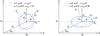 |
Fig. 1 Illustrations of the noise distribution in the (Q, U) plane. The solid and dashed blue lines represent the 1σ probability contours around the true polarization values (Q0, U0), also parameterized by (p0, ψ0). Left: the canonical case (ε = 1, ρ = 0) is shown as a solid line. The dashed line shows the introduction of a correlation ρ = 0.5, leading to an effective ellipticity (εeff> 1) rotated by an angle θ. Right: same transformation, starting from the elliptical case (ε = 2, ρ = 0). |
2. (p, ψ) probability density functions
2.1. Notation
The goal of this paper is to characterize the distribution of naïve polarization measurements, given the true polarization parameters and their associated noise estimates. We denote the true values by (I0, Q0, U0), representing the true total intensity and Stokes linear polarization parameters, and with  . The quantities (I, Q, U) are the same for the measured values. The polarization fraction and polarization angle are defined by
  (1)for the true values and
  (2)for the measurements. The true Stokes parameters can be expressed by Q0 ≡ p0I0 cos(2ψ0) and U0 ≡ p0I0 sin(2ψ0), while for the measurements Q ≡ pI cos(2ψ) and U ≡ pI sin(2ψ). Although the true intensity I0 is strictly positive, the measured intensity I may be negative due to noise, thus I0 can take values between 0 and + ∞, while I ranges between − ∞ and + ∞. The measured Stokes parameters Q and U are real, finite quantities, ranging from − ∞ to + ∞, that with the addition of noise do not necessarily satisfy the relation Q2 + U2 ≤ I2 obeyed by the underlying quantities, i.e.,
  . The true polarization fraction p0 can take values in the range 0 to 1, while the measured polarization fraction p ranges between − ∞ and + ∞. Finally we define ψ0 and ψ such that they are both defined in the range [−π/ 2, + π/ 2 ].
Previous studies of polarization measurements usually made strong assumptions concerning the noise properties, in particular: (i) correlations between the total and polarized intensities were neglected; (ii) correlated noise between Q and U was also neglected; and (iii) equal noise was assumed on Q and U measurements. We propose instead to use the full covariance matrix defined by 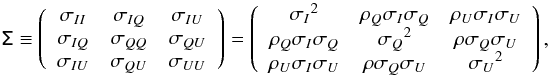 (3)where σXY is the covariance of the two random variables X and Y, and the following quantities are usually introduced in the literature to simplify the notation:
  (4)Here ε is the ellipticity between the Q and U noise components, and ρ (which lies between − 1 and + 1) is the correlation between the Q and U noise components. Similarly, ρQ and ρU are the correlations between the noise in intensity I and the Q and U components, respectively.
The parameterization just described could be misleading, however, since the ellipticity ε does not represent the effective ellipticity in the (Q, U) plane if the correlation is not zero. This is illustrated in Fig. 1 for two initial values of the ellipticity ε. A new reference frame (Q′, U′) where the Stokes parameters are now uncorrelated can always be obtained through rotation by an angle  (5)We can calculate the covariance matrix in the rotated frame by taking the usual R Σ RT. In this new reference frame, the errors on Q′ and U′ are uncorrelated and defined as
 ![Mathematical equation: \begin{equation} \begin{array}{l} \sigma_{Q^\prime}^2 = \sigma_{ Q}^2 \cos^2\theta + \sigma_{ U}^2 \sin^2 \theta + \sigma_{ QU} \sin 2\theta , \\[2mm] \sigma_{U^\prime}^2 = \sigma_{ Q}^2 \sin^2\theta + \sigma_{ U}^2 \cos^2 \theta - \sigma_{ QU} \sin 2\theta , \end{array} \end{equation}](/articles/aa/full_html/2015/02/aa22271-13/aa22271-13-eq45.png) (6)so that the effective ellipticity εeff is now given by
(6)so that the effective ellipticity εeff is now given by  (7)where
  (8)When expressed as a function of the (ε, ρ) parameters, we obtain
 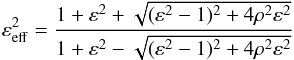 (9)and
 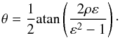 (10)This parameterization of the covariance matrix Σ in terms of εeff and θ is preferred in our work for two reasons. Firstly, the shape of the noise distribution in the (Q, U) space is now contained in a single parameter, the effective ellipticity εeff (≥ 1), instead of two parameters, ε and ρ. Secondly, the noise distribution is now independent of the reference frame. This is also related to the fact that the properties of the noise distribution do not depend on three (I0, p0, ψ0) plus six (from Σ) parameters, but only on eight, since it actually only depends on the difference in the angles 2ψ0 − θ, which simplifies the analysis quite a lot. For what follows we also define det(Σ) = σ6 as the determinant of the covariance matrix.
2.2. 3D probability density functions
The probability density function (PDF) gives the probability of obtaining a set of values (I, Q, U), given the true Stokes parameters (I0, Q0, U0) and the covariance matrix Σ. As a short cut, we refer to this as the “3D PDF”. When Gaussian noise is assumed for each Stokes component, this distribution in the space (I, Q, U) is given by 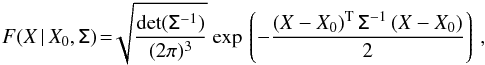 (11)where X and X0 are the vectors of the Stokes parameters [ I,Q,U ] and [ I0,Q0,U0 ], Σ-1 is the inverse of the covariance matrix (also called the “precision matrix”), and det(Σ-1) = σ-6 is the determinant of Σ-1. This definition ensures that the probability density function is normalized to 1. The iso-probability surfaces in the (I, Q, U) space are ellipsoids.
Using normalized polar coordinates, the probability density function f(I,p,ψ | I0,p0,ψ0,Σ) can be computed explicitly. However, the expression (see Eq. (A.1)) is a little cumbersome, so we have put it in Appendix A. We point out the presence of a factor 2 | p | I2 in front of the exponential, coming from the Jacobian of the transformation.
2.3. 2D marginal (p,ψ) distribution
We compute the 2D probability density function f2D(p,ψ) by marginalizing the probability density function f(I,p,ψ) (see Eq. (A.1)) over intensity I on the range − ∞ to + ∞. The computation is quite straightforward (see Appendix B), leading to an expression that depends on the sign of p, given in Eqs. (A.2) and (A.3).
In many cases, two further assumptions can be made: (i) the correlations between I and (Q, U) is negligible, i.e., ρQ = ρU = 0; and (ii) the S/N of the intensity I0/σI is so high that I can be considered to be perfectly known, yielding I = I0, as discussed in Quinn (2012). Making such assumptions allows us to reduce the covariance matrix Σ to a 2 × 2 matrix, Σp, which we define as 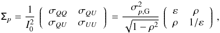 (12)where σp,G is defined by
  , leading to
 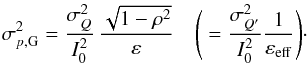 (13)This parameter σp,G is linked to the normalization of the 2D distribution, because it represents the radius of the equivalent spherical Gaussian distribution that has the same integrated area as the elliptical Gaussian distribution. The probability density function f2D can then be simplified, as given in Eq. (A.4). The matching between the two expressions for f2D, Eqs. (A.2)−(A.4), when I0/σI → ∞, is ensured simply by the consistency of the determinants of Σ and Σp, when ρQ = ρU = 0:
  (14)We also recall that in the canonical case (εeff = 1), the probability density function can be simplified to
 ![Mathematical equation: \begin{equation} f_{\rm 2D} = \frac{p}{\pi \sigma_{ p}^2} \, \mathrm{exp} \left \{-\frac{1}{2\sigma_{ p}^2} \left[p^2 + p_0^2 - 2pp_0\cos2(\psi-\psi_0) \right] \right\} , \end{equation}](/articles/aa/full_html/2015/02/aa22271-13/aa22271-13-eq80.png) (15)where σp,G also simplifies to σp = σQ/I0 = σU/I0. We provide illustrations of the 2D PDFs in Appendix C.
(15)where σp,G also simplifies to σp = σQ/I0 = σU/I0. We provide illustrations of the 2D PDFs in Appendix C.
2.4. 1D marginal p and ψ distributions
The marginal probability density functions of p and ψ can be obtained by integrating the 2D PDF given by Eq. (A.4) over ψ (between − π/ 2 and + π/ 2) and p (between 0 and + ∞), respectively, when assuming the S/N on the intensity to be infinite. These two probability density functions theoretically depend on p0, ψ0, and Σp. While the expressions obtained in the general case (Aalo et al. 2007) are provided in Appendix D, the expression for the marginal p distribution reduces to the Rice law (Rice 1945) when ε = 1 and ρ = 0: 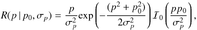 (16)where ℐ0(x) is the zeroeth-order modified Bessel function of the first kind (Abramowitz & Stegun 1964). This expression no longer has a dependence on ψ0. With the same assumptions, the marginal ψ distribution (extensively studied in Naghizadeh-Khouei & Clarke 1993) is given by
 ![Mathematical equation: \begin{equation} G(\psi\, |\, p_0,\psi_0,\sigma_{ p}) = \frac{1}{\sqrt{\pi}} \left\{ \frac{1}{\sqrt{\pi}} + \eta_0{\rm e}^{\eta_0^2} \left[ 1+ \mathrm{erf}(\eta_0) \right] \right\} {\rm e}^{-p_0^2I_0^2/2\sigma_{ p}^2}, \end{equation}](/articles/aa/full_html/2015/02/aa22271-13/aa22271-13-eq89.png) (17)where
(17)where  . This distribution depends on p0 and is symmetric about ψ0.
3. Impact of the covariance matrix on the bias
We now quantify how the effective ellipticity of the covariance matrix affects the bias of the polarization measurements, compared to the canonical case. We would like to determine under what conditions the covariance matrix may be simplified to its canonical expression, in order to minimize computations. The impact of the correlation and the ellipticity of the covariance matrix are first explored in the 2D (p, ψ) plane with infinite intensity S/N. The cases are then investigated of finite S/N on intensity and of the correlation between total and polarized intensity.
3.1. Methodology
Given a collection of measurements of the same underlying polarization parameters (p0, ψ0), we build the statistical bias on p and ψ by averaging the discrepancies  and
and  (always defining the quantity ψ − ψ0 between − π/ 2 and + π/ 2). With knowledge of the probability density function f2D(p,ψ | p0,ψ0,Σp), we can obtain the statistical bias directly by computing the mean estimates
  (18)and
  (19)Here
  and
and  are the mean estimates from the probability density function, defined as the first moments of f2D:
 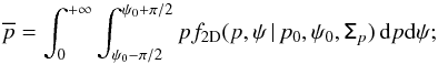 (20)and
  (21)To quantify the importance of this bias, we can compare it to the dispersion of the polarization fraction and angle measurements, σp,0 and σψ,0. These are defined as the second moments of the probability density function f2D:
  (22)and
  (23)Here subscript 0 signifies that this dispersion has been computed using full knowledge of the true polarization parameters and the associated probability density function.
We chose σp,G introduced in Sect. 2.3 as our characteristic estimate of the polarization fraction noise in its relationship to the covariance matrix Σp. This is used to define the S/N of the polarization fraction p0/σp,G, which is kept constant when exploring the ellipticity and correlation of the Q − U components. In Sect. 4 we discuss how robust this estimate is against the true dispersion σp,0.
We define three specific setups of the covariance matrix to investigate: (i) the canonical case, εeff = 1, equivalent to ε = 1, ρ = 0; the low regime, 1 ≤ εeff< 1.1; and the extreme regime, 1 ≤ εeff< 2. These are used in the rest of this paper to quantify departures of the covariance matrix from the canonical case and to characterize the impact of the covariance matrix on polarization measurements in each regime. It is worth recalling that to each value of the effective ellipticity εeff there corresponds a set of equivalent parameters ε, ρ, and θ. The average level of the effective ellipticity εeff in the Planck data over the full sky on a one-degree scale has been estimated around 1.12 (Planck Collaboration IntSPlanck Collaboration Int. XIX 2014), which lies at the limit of the low regime. This does not prevent observing higher effective ellipticities in specific regions of the sky, which could fall in the extreme regime.
3.2. Q–U ellipticity
We assume here that the intensity is perfectly known and that there is no correlation between the total intensity I and the polarized intensity, so that I = I0 and ρQ = ρU = 0. In this case we can now refer to Eq. (A.4) for the 2D probability density function.
Unlike the canonical case, where the effective ellipticity differs from εeff = 1, the statistical biases on the polarization fraction and angle become dependent on the true polarization angle ψ0, as illustrated in Fig. 2 for the special case of θ = 0 (no correlation). For extreme values of the ellipticity (e.g., εeff = 2), the relative bias on p oscillates between 0.9 and 1.5 times the canonical bias (εeff = 1). These oscillations with ψ0 quickly vanish when the ellipticity gets closer to 1, as shown for εeff = 1.1 in the figure. The presence of correlations (i.e., ρ ≠ 0) increases the effective ellipticity of the noise distribution associated with a global rotation, as detailed in Sect. 2.1. Thus correlations induce the same oscillation patterns as observed in Fig. 2 for an effective ellipticity larger than 1 and a null correlation, but amplified at the corresponding effective ellipticity εeff and shifted by an angle θ/ 2, according to Eqs. (9) and (10), respectively.
The top panel of Fig. 3 shows the dependence of the polarization fraction bias on the effective ellipticity for three levels of S/N, p0/σp,G = 1, 2, and 5, and including the full range of true polarization angle ψ0. The figure indicates the variability interval of Δp/σp,0 for each ellipticity, for changes in ψ0 over the range − π/ 2 to π/ 2. We observe that the higher the S/N, the stronger the relative impact of the ellipticity compared to the canonical case. In the low regime the relative bias to the dispersion increases from 9% to 12% (compared to 10% in the canonical case) at a S/N of 5, while it spans from 69% and 73% (around the 71% of the canonical case) at a S/N of 1. In the low regime, therefore, the impact of the ellipticity on the bias of the polarization fraction represents only about 4% of the dispersion, regardless of the S/N, which can therefore be neglected. However, in the extreme regime, the impact of the ellipticity can go up to 33% at intermediate S/N (~ 2), which can no longer be neglected.
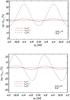 |
Fig. 2 Impact of the initial true polarization angle ψ0 and of varying effective ellipticity εeff on the relative polarization fraction bias Δp/σp,0 (top) and the relative polarization angle bias Δψ/σψ,0 (bottom). We assume no correlation here, so that θ = 0, and we set the S/N to p0/σp,G = 2. The canonical case (εeff = 1) is shown by the red line. |
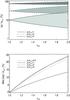 |
Fig. 3 Impact of the effective ellipticity εeff on the levels of bias. Top: Δp/σp,0 as a function of the effective ellipticity εeff, displayed for three levels of the S/N, p0/σp,G = 1, 2, and 5. The grey shaded regions indicate the whole extent of variability due to ψ0 and θ spanning the range − π/ 2 to π/ 2. Bottom: maximum | Δψ | /σψ,0 value for ψ0 and θ spanning the range − π/ 2 to π/ 2, plotted as a function of the effective ellipticity εeff, displayed for four levels of the S/N, p0/σp,G = 0.5, 1, 2, and 5. |
Concerning the impact on polarization angle – while no bias occurs in the canonical case, some oscillations in the bias Δψ with ψ0 appear as soon as εeff> 1. The amplitude can reach up to 24% of the dispersion in the extreme regime and up to 4% in the low regime, as illustrated in the bottom panel of Fig. 2. Again, these oscillations are shifted and amplified in the presence of correlations between the Stokes parameters, compared to the case with no correlation. As an overall indicator, in the bottom panel of Fig. 3 we provide the maximum bias Max | Δψ | normalized by the dispersion σψ,0 over the full range of ψ0 as a function of the ellipticity. This quantity barely exceeds 24% (i.e., ~ 9°) in the worst case, i.e., for εeff = 2 and low S/N, and it falls to below 4% (i.e., ~ 1.5°) in the low regime. Thus the bias on ψ always remains well below the level of the true uncertainty on the polarization angle at the same S/N (see Sect. 4), so that the bias of the polarization angle induced by an ellipticity εeff> 1 can be neglected to first order for the low regime of the ellipticity, i.e., when there is less than a 10% departure from the canonical case.
3.3. I uncertainty
The uncertainty in the total intensity I has two sources: the measurement uncertainty expressed in the covariance matrix, and an astrophysical component of the uncertainty due to the imperfect characterization of the unpolarized contribution to the total intensity. This second source can be seen, for instance, with the cosmic infrared background in Planck data: its unpolarized emission can be viewed as a systematic uncertainty on the total intensity (dominated by the Galactic dust thermal emission), when one is interested in the polarization fraction of the Galactic dust. To retrieve the actual polarization fraction, it is necessary to compute it through 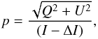 (24)where ΔI is the unpolarized emission, which is imperfectly known. The uncertainty σΔI on this quantity can be viewed as an additional uncertainty σI on the total intensity, and therefore the S/N has to be written I0/σI = (I − ΔI) /σΔI.
To consider the effects on polarization quantities, we first recall that, because of its definition, the measurement of polarization angle ψ is not affected by the uncertainty on intensity (when no correlation exists between I and Q and U), contrary to the polarization fraction p, which is defined as the ratio of the polarized intensity to the total intensity. Thus the uncertainty of the total intensity does not induce any bias on ψ.
To quantify the influence of a finite S/N I0/σI on the bias of p, we compute the mean polarization fraction over the PDF: 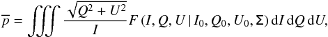 (25)with F given by Eq. (11). We write it this way, because using f2D given by Eqs. (A.2) and (A.3) would lead to both positive and negative logarithmic divergences for p → ± ∞ (related to samples for which I → 0). These divergences can be shown to be artificial by using the Gaussian PDF of (I,Q,U) instead of f2D.
The presence of noise in total intensity measurements increases the absolute bias  , as shown in Fig. 4, where Δp, normalized by the true value p0, is plotted as a function of the S/N I0/σI. This is shown for three levels of the polarization S/N p0/σp,G = 1, 2, and 5, and the three regimes of the covariance matrix, assuming that ρQ = ρU = 0.
The bias may be enhanced by a factor of 1.5 to 4 times p0 when the S/N on I goes from infinite (i.e., perfectly known I) to about 2. It then drops again for lower S/N, which is the result of the increasing number of negative p samples. We only consider the domain where (I0/σI) > (p0/σp,G).
Comparison of the bias to the dispersion σp,0, as was done in the previous section, is not straightforward when the total intensity is uncertain. This is because the integral defining σp,0 (see Eq. (22)) has positive linear divergences for p → ± ∞. Unlike the case of , this divergence cannot be alleviated by working in (I,Q,U) space.
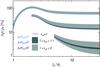 |
Fig. 4 Polarization fraction bias, normalized to the true value p0, as a function of the S/N I0/σI, plotted for three values of the polarization S/N, p0/σp,G, and values of the effective ellipticity εeff covering the canonical (full line), low (dark grey shaded region), and extreme (light grey shaded region) regimes of the covariance matrix. The intensity correlation coefficients are set to ρQ = ρU = 0. We only consider the domain where (I0/σI) > (p0/σp,G). |
To overcome this we therefore used a proxy  , which is the dispersion of p computed on a subset of (I,Q,U) space that excludes total intensity values below ωI0, with ω = 10-7. This threshold is somewhat arbitrary, as increases linearly with 1 /ω. The value 10-7 is merely meant to serve as an illustration. Figure 5 shows
  as a function of I0/σI for the same values of the polarization S/N p0/σp,G and the same regimes of the covariance matrix as in Fig. 4. At high S/N for I, we asymptotically recover the values obtained in the top panel of Fig. 3. As long as I0/σI> 5, the relative bias on p is barely affected by the uncertainty on the intensity, especially for low polarization S/N, p0/σp,G. A minor trend is still seen in the range 5 <I0/σI< 10 for p0/σp,G = 5. The relative bias may be enhanced by a factor of around 2 in that case, when the S/N on intensity and polarization are ~5. However, this situation is unlikely to be observed in astrophysical data, since the uncertainty on total intensity is usually much less than for polarized intensity.
Contrary to these high S/N (I0/σI> 5) features, which are quite robust with respect to the choice of threshold ωI0, the drop in relative bias at lower intensity S/N, i.e., I0/σI< 5, is essentially due to the divergence of the dispersion of p. This part of Fig. 4 should thus be taken as nothing more than an illustration of the divergence at low S/N for I. It should be stressed, however, that this increase in the dispersion of p has to be carefully considered when dealing with low S/N intensity data, which can be the case well away from the Galactic plane.
 |
Fig. 5 Same as Fig. 4, but showing the bias on the polarization fraction relative to the dispersion proxy |
3.4. Correlation between I and Q–U
With non-zero noise on total intensity, it becomes possible to explore the effects of the coefficients ρQ and ρU, corresponding to correlation between the intensity I and the (Q,U) plane. We first note that introducing correlation parameters ρQ and ρU that are different from zero directly modifies the ellipticity ε and correlation ρ between Stokes Q and U. Simple considerations on the Cholesky decomposition of the covariance matrix Σ (given in Appendix E) show that for a given ellipticity ε and correlation parameter ρ, obtained when ρQ = ρU = 0, the ellipticity ε′ and correlation ρ′ become 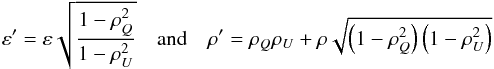 (26)when ρQ and ρU are no longer zero. Consequently, non-zero ρQ and ρU lead to similar impacts as found for a non-canonical effective ellipticity (εeff ≠ 1), discussed in Sect. 3.2. Moreover, to investigate the sole impact of non-zero ρQ and ρU with a finite S/N on the intensity, we have compared the case (ε,ρ,ρQ,ρU) to the reference case (ε′,ρ′,0,0). We find that the relative change of the polarization fraction bias Δp is at most 10–15% over the whole range of I0/σI explored in this work (i.e.,
  ).
).
The difference between the polarization angle bias computed for (ε,ρ,ρQ,ρU) and for the reference case (ε′,ρ′,0,0) is at most Δψ − Δψref ~ 4° and essentially goes to zero above I0/σI ~ 2–3. The dependence of the change in bias with (ρQ,ρU) is similar to the one for Δp/ Δpref, except that it depends solely on ρU for ψ0 = 0 and solely on ρQ for ψ0 = π/ 4.
4. Polarization uncertainty estimates
If we are given the polarization measurements and the noise covariance matrix of the Stokes parameters, we would like to derive estimates of the uncertainties associated with the polarization fraction and angle. These are required to (i) define the S/N of these polarization measurements and to (ii) quantify how important the bias is compared to the accuracy of the measurements. In the most general case, the uncertainties in the polarization fraction and angle do not follow a Gaussian distribution, so that confidence intervals should be used properly to obtain an estimate of the associated errors, as described in Sect. 4.5. However, it can sometimes be assumed as a first approximation that the distributions are Gaussian, in order to derive quick estimates of the p and ψ uncertainties, defined as the variance of the 2D distribution of the polarization measurements. We explore below the extent to which this approximation can be utilized, when using the most common estimators of these two quantities.
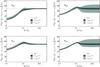 |
Fig. 6 Probability |
![Mathematical equation: \hbox{$[p-\sigma_{ p}^{\rm low}, p+\sigma_{ p}^{\rm up}]$}](/articles/aa/full_html/2015/02/aa22271-13/aa22271-13-eq176.png)


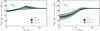 |
Fig. 7 Same as Fig. 6, but for the polarization angle uncertainty estimators. Left: σψ,0. Right: conventional σψ,C. |
4.1. Standard deviation estimates
To compare the robustness of the uncertainty estimates, we build 10 000 Monte Carlo simulated measurements in each of the three regimes of the covariance matrix (canonical, low, and extreme), by varying the S/N of p and the polarization angle ψ0 inside the range − π/ 2 and π/ 2. We use the simulations to compute the posterior fraction of measurements for which the true value p0 or ψ0 falls inside the ± σ range around the measurement. This provides the probability  shown in Figs. 6 and 7 for p and ψ, respectively.
We first focus on the true uncertainty estimates, as defined in Sect. 3.1. We observe that the σp,0 true estimates (top left of Fig. 6) fall below the Gaussian value  (i.e., 68%) once the S/N goes below 3. The σψ,0 true estimates (left of Fig. 7) provide conservative probabilities (
 ) for S/N> 0.5. This is also shown in Fig. 8 as a function of the S/N, for the canonical, low, and extreme regimes of the covariance matrix. It is not strongly dependent on the ellipticity of the covariance matrix. It shows a maximum of
  at low S/N, and converges slowly to 0 at high S/N (still ~ 10° at S/N = 3). Thus we might imagine using such estimates as reasonably good approximations of the uncertainties at high S/N (> 3) for p, and over almost the entire range of S/N for ψ. However, these true p and ψ uncertainties, σp,0 and σψ,0, respectively, depend on p0 and ψ0, which remain theoretically unknown. Thus we can only provide specific estimates of those variance quantities, as explained below.
4.2. Geometric and arithmetic estimators
Two estimates of the polarization fraction uncertainty can be obtained independently of
the measurements themselves, which makes them easy to compute: (i) the geometric
(σp,G) estimate; and
(ii) the arithmetic (σp,A) estimate. The
geometric estimator has already been introduced earlier when we derived the expression for
the 2D (p,ψ)
PDF f2D. It is defined via the determinant of
the 2D covariance matrix Σp as
, with its
expression given in Eq. (13). We recall
that the determinant of the covariance matrix Σp is linked to the area inside a
probability contour and independent of the reference frame of the Stokes parameters. In
the canonical case, this estimate gives back the usual expressions, σp,G =
σQ/I0
=
σU/I0,
used to quantify the noise on the polarization fraction. It can be considered as the
geometric mean of σQ and
σU when there is no
correlation between them; i.e.,  .
.
The arithmetic estimator is defined as a simple quadratic mean of the variance in
Q and
U:
 (27)This estimate also gives
back σp,A =
σQ/I0
=
σU/I0
in the canonical case. Furthermore, it is also independent of the reference frame or of
the presence of correlations.
(27)This estimate also gives
back σp,A =
σQ/I0
=
σU/I0
in the canonical case. Furthermore, it is also independent of the reference frame or of
the presence of correlations.
The two estimators have very similar behaviour, as can be seen in the top and bottom
right-hand panels of Fig. 6. They agree perfectly
with a 68% confidence level for S/N p0/σp,0>
4 and for standard simplification of the covariance matrix. Both
estimators provide conservative probability ( ) in
the S/N range 0.5−4. The
impact of the effective ellipticity of the covariance matrix (grey shaded area) is
stronger for higher values of the S/N (>2) and can yield variations of 30% in the
probability
for the extreme regime. These estimators should be used cautiously for
high ellipticity, but provide quick and conservative estimates in the other cases.
) in
the S/N range 0.5−4. The
impact of the effective ellipticity of the covariance matrix (grey shaded area) is
stronger for higher values of the S/N (>2) and can yield variations of 30% in the
probability
for the extreme regime. These estimators should be used cautiously for
high ellipticity, but provide quick and conservative estimates in the other cases.
4.3. Conventional estimate
The conventional determination of the uncertainties proposed by Serkowski (1958, 1962) is often used for polarization determinations based on optical extinction data. Although investigated by Naghizadeh-Khouei & Clarke (1993), these conventional uncertainties still do not include asymmetrical terms and correlations in the covariance matrix. Here we extend the method to the general case by using the derivatives of p and ψ around the observed values of the I, Q, and U parameters. It should be noted that, since this approach is based on derivatives around the observed values of (I, Q, U), it is only valid in the high S/N regime. The detailed derivation, provided in Appendix F, leads to the expressions 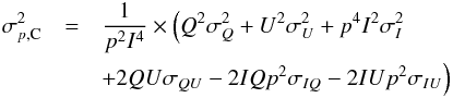 (28)and
 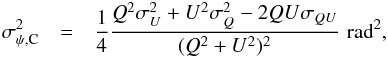 (29)where I, Q, U, and p are the measured quantities, and σXY are the elements of the covariance matrix. We recall that the maximum uncertainty on ψ is equal to
  (integral of the variance of the polarization angle over a flat distribution between − π/ 2 and π/ 2). When σI can be neglected, we obtain
  (30)Because the uncertainty of ψ is also often expressed in degrees, we provide the associated conversions:
  and
and  . Moreover, under the canonical assumptions, we recover σp,C = σp,G = σQ/I0 = σU/I0 and σψ,C = σp,C/ 2p rad.
 |
Fig. 8 True polarization angle uncertainty, σψ,0, as a function of the S/N, p0/σp,G. The three regimes (canonical, low, and extreme) of the covariance matrix are explored (solid line, light, and dark grey shaded regions, respectively). |
Since the conventional estimate of the uncertainty σp,C is equal to σp,G under the standard simplifications of the covariance matrix, it has the same deficiency at low S/N (see bottom left-hand panel of Fig. 6). The impact of the effective ellipticity of the covariance matrix tends to be negligible at high S/N (p0/σp,G> 4) and remains limited at low S/N. Thus this estimator of the polarization fraction uncertainty appears more robust than the geometric and arithmetic estimators, while still being easy to compute and valid (even conservative) over a wide range of S/N.
The conventional estimate of the polarization angle uncertainty, σψ,C, is shown in Fig. 7 (right-hand panel) in the canonical, low, and extreme regimes of the covariance matrix. It appears that σψ,C is strongly under-estimated at low S/N, mainly due to the presence of the term 1 /p in Eq. (30), where p is strongly biased at low S/N. For S/N> 4, the agreement between the probability and the expected value is good, while the impact of the ellipticity of the covariance matrix becomes negligible only for S/N> 10. This estimator can certainly be used at high S/N.
 |
Fig. 9 Probability density function (PDF) of the measured S/N p/σp,G (where σp,G is the geometric estimate) as a function of the true S/N p0/σp,0, with no ellipticity and correlation in the covariance matrix Σp. The mean likelihood, |
4.4. S/N estimates
It is important to stress how any measurement of the S/N p/σp,G is strongly affected by the bias on the measured polarization fraction p, as shown in Fig. 9. We observe that at high S/N (p0/σp,0> 2), the measured S/N, here p/σp,G, is very close to the true S/N. The mean likelihood of the measured S/N (solid line) flattens for lower true S/N, such that  tends to
  for p0/σp,0< 1, which comes from the limit of the Rice (1945) function when p0/σp,0 → 0. This should be taken into account carefully when dealing with polarization measurements at intermediate S/N. For any measurement with a S/N p0/σp,0< 2, it is in fact impossible to obtain an estimate of the true S/N, because this is fully degenerate owing to the bias of the polarization fraction.
4.5. Confidence intervals
We have seen the limitations of the Gaussian assumption for computing valid estimates of the polarization uncertainties. To obtain a robust estimate of the uncertainty in p and ψ at low S/N, one has to construct the correct confidence regions or intervals. The λ% confidence interval around a measurement p is defined as the interval that has a probability of containing the true value p0 exactly equal to λ/ 100, where (1 − λ) is called “critical parameter”. This interval is constructed from the PDF and does not require any estimate of the true polarization parameters. Mood & Graybill (1974), Simmons & Stewart (1985), and Vaillancourt (2006) have provided a simple way to construct such confidence intervals for the polarization fraction p when the usual simplifications of the covariance matrix are assumed. Naghizadeh-Khouei & Clarke (1993) provide estimates of the confidence intervals for the polarization angle ψ under similar assumptions, and this is even simpler, because in that case fψ(ψ | p0,ψ0,Σp) only depends on the S/N p0/σp,0.
Once the covariance matrix is allowed to include ellipticity and correlations, we see in Sect. 2.4 and Appendix D how the marginalized PDFs fp(p | p0,ψ0,Σp) and fψ(ψ | p0,ψ0,Σp) depend on the true polarization fraction p0 and the true polarization angle ψ0. This leads us to consider ψ0 as a “nuisance parameter” when building confidence intervals of p0, and vice-versa. We propose below an extension of the Simmons & Stewart (1985) technique, using an iterative method to build the confidence intervals of p0 and ψ0 simultaneously.
For each possible value of p0 and ψ0 (spanning the range 0 to 1, and − π/ 2 to π/ 2, respectively), we compute the quantities p−, p−, ψ−, and ψ−, which provide the lower and upper limits in p and ψ of the region Ω(λ,p0,ψ0) defined by  (31)such that the contour of the region Ω is an iso-probability contour of the PDF f2D. We stress that the choice of a confidence interval is still subjective and may be shifted by any arbitrary value of p or ψ, provided that the integral over the newly defined region is also λ/ 100. The definition we have chosen ensures that the region Ω(λ,p0,ψ0) is the smallest possible. We also note that
  (32)which implies that the rectangular region bounded by p−, p−, ψ−, and ψ− is a conservative choice. For a given λ and covariance matrix Σp, we can finally obtain a set of four upper and lower limits on p and ψ: p−(p0,ψ0); p−(p0,ψ0); ψ−(p0,ψ0); and ψ−(p0,ψ0). We illustrate this with the example of (p, ψ) set to (0.1, π/8) in Fig. 10. For given polarization measurements (p, ψ), we trace the loci p−(p0,ψ0) = p (dashed line), p−(p0,ψ0) = p (dot-dash line), ψ−(p0,ψ0) = ψ (long dashed line), and ψ−(p0,ψ0) = ψ (dash-dot-dot-dot line). Finally, the 68% confidence intervals
 ![Mathematical equation: \hbox{$[p_0^{\rm low},p_0^{\rm up}]$}](/articles/aa/full_html/2015/02/aa22271-13/aa22271-13-eq248.png) of p0 and [
of p0 and [![Mathematical equation: \hbox{$\psi_0^{\rm low},\psi_0^{\rm up}]$}](/articles/aa/full_html/2015/02/aa22271-13/aa22271-13-eq249.png) of ψ0 are defined by building the smallest rectangular region (solid line in Fig. 10) that simultaneously covers the domain in p0 and ψ0 between the upper and lower limits defined above and which satisfies the conditions:
of ψ0 are defined by building the smallest rectangular region (solid line in Fig. 10) that simultaneously covers the domain in p0 and ψ0 between the upper and lower limits defined above and which satisfies the conditions: ![Mathematical equation: \begin{eqnarray} p_0^{\rm low} &=& \mathrm{min}_{p_0} \left(\: p=p^{-} \left\{ p_0\: , \: \psi_0 \in [\psi_0^{\rm low},\psi_0^{\rm up}] \right\} \: \right ); \nonumber \\ p_0^{\rm up} &=& \mathrm{max}_{p_0} \left( \: p = p_{-} \left\{ p_0\: , \: \psi_0 \in [\psi_0^{\rm low} ,\psi_0^{\rm up}] \right\} \: \right ); \nonumber \\ \psi_0^{\rm low}&=& \mathrm{min}_{\psi_0} \left( \: \psi = \psi^{-} \left\{ p_0 \in [p_0^{\rm low}, p_0^{\rm up} ] \: , \: \psi_0\right\} \: \right ); \nonumber \\ \psi_0^{\rm up}&=& \mathrm{max}_{\psi_0} \left( \: \psi = \psi_{-} \left\{ p_0 \in [p_0^{\rm low}, p_0^{\rm up} ] \: , \: \psi_0\right\} \: \right ). \end{eqnarray}](/articles/aa/full_html/2015/02/aa22271-13/aa22271-13-eq250.png) (33)Using these conditions, the confidence interval of p0 takes the nuisance parameter ψ0 over its own confidence interval into account, and vice-versa. This has to be constructed iteratively, starting with
(33)Using these conditions, the confidence interval of p0 takes the nuisance parameter ψ0 over its own confidence interval into account, and vice-versa. This has to be constructed iteratively, starting with  and
and  , to build first guesses for
  and
and  , which are then used to build a new estimate of the confidence intervals of ψ0, and so on until convergence. In practice, it converges very quickly. We emphasize that these confidence intervals are conservative, because they include the impact of the nuisance parameters, implying that
  (34)regardless of the true values p0, ψ0.
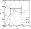 |
Fig. 10 Construction of 68% confidence intervals |
![Mathematical equation: \hbox{$[\psi_0^{\rm low},\psi_0^{\rm up}]$}](/articles/aa/full_html/2015/02/aa22271-13/aa22271-13-eq256.png)
5. Summary
This paper represents the first step in an extensive study of polarization analysis methods. We focused here on the impact of the full covariance matrix on naïve polarization measurements and especially the impact on the bias. We derived analytical expressions for the PDF of the polarization parameters (I,p,ψ) in the 3D and 2D cases, taking the full covariance matrix Σ of the Stokes parameters I, Q, and U into account.
The asymmetries of the covariance matrix can be characterized by the effective ellipticity εeff, expressed as a function of the ellipticity ε and the correlation ρ between Q and U in a given reference frame, and by the correlation parameters ρQ and ρU between the intensity I and the Q and U parameters. We quantified departures from the canonical case (εeff = 1), which are usually assumed in earlier works on polarization. We explored this effect for three regimes of the covariance matrix: the canonical case (εeff = 1); the low regime, 1 <εeff< 1.1; and the extreme regime 1 <εeff< 2. We first emphasized the impact of the true polarization angle ψ0, which can produce variations in the polarization fraction bias of up to 30% of the dispersion of p, in the extreme regime, and up to 5% in the low regime. We then estimated the statistical bias on the polarization angle measurement ψ. This can reach up to 9° when the ellipticity or the correlation between the Q and U Stokes components becomes important (εeff ~ 2) and the S/N is low. However, when values of the effective ellipticity are in the low regime (i.e., less than 10% greater than the canonical values) the bias on ψ remains limited (i.e., < 1°), and well below the level of the measurement uncertainty (by a factor of 5–25). Thus the bias on ψ can be neglected, to first order, for small departures of the covariance matrix from the canonical case.
On the other hand, we quantified the impact of the uncertainty of the intensity on the relative and absolute statistical bias of the polarization fraction and angle. We provided the modified PDF in (p,ψ) arising from a finite S/N of the intensity, I0/σI. We showed that, above an intensity S/N of 5, the relative bias on the polarization fraction p generally remains unchanged at polarization S/N p0/σp,G< 2, while it is slightly enhanced when the intensity and the polarization S/N lie in the intermediate range, p0/σp,G> 2. For S/N of the intensity I0/σI below 5, the relative bias on p suddenly drops to 0, because of the increasing dispersion. Indeed, the absolute bias can be higher by a factor as large as 5 when the S/N on I drops below 2 to 3; this is associated with a dramatic increase in the dispersion of the polarization fraction, which diverges and strongly overwhelms the increase of the bias at low S/N. The uncertainty of the intensity thus has to be taken into account properly when analysing polarization data for faint objects, in order to derive the correct polarization fraction bias and uncertainty. Similarly, the case of faint polarized objects on top of a varying but unpolarized background can lead to a question about the correct intensity offset to subtract, yielding an effective additional uncertainty on the intensity.
The impact of correlations between the intensity and the Q and U components has also been quantified in the case of a finite S/N on the intensity. It has been shown that the bias on p is only slightly affected (below 10% difference compared with the canonical case) even at low S/N on I, when the correlations ρQ and ρU span the range − 0.2 to 0.2.
We have additionally addressed the question of how to obtain a robust estimate of the uncertainties on polarization measurements (p,ψ). We extended the often-used procedure of Simmons & Stewart (1985) by building confidence intervals for polarization fraction and angle simultaneously, taking the full properties of the covariance matrix into account. This method makes it possible to build conservative confidence intervals around polarization measurements.
We have explored the domain of validity for the commonly used polarization uncertainty estimators based on the variance of the PDF (assuming a Gaussian distribution). The true dispersion of the polarization fraction has been shown to provide robust estimates only at high S/N (above 3), while the true dispersion of the polarization angle yields conservative estimates for S/N> 0.5. Simple estimators, such as the geometric and arithmetic polarization fraction uncertainties, appear sensitive to the effective ellipticity of the covariance matrix at high S/N, while they provide conservative estimates over a wide range of S/N (above 0.5) in the canonical case. The conventional method, usually adopted to analyse optical extinction polarization data, provides the most robust estimates of σp for S/N above 0.5, with respect to the ellipticity of the covariance matrix, but poor estimates of σψ, which are valid only at very high S/N (above 5).
We have seen how much the naïve polarization estimates provide poor determinations of the true polarization parameters and how it can be difficult to recover the true S/N of a measurement. In a companion paper (Montier et al. 2015), we review different estimators of the true polarization from experimental measurements that partially correct this bias
in p and ψ, using full knowledge of the polarization covariance matrix.
Online material
Appendix A: Expressions for PDFs
Here we present expressions for the 2D PDFs that are discussed in Sect. 2:
![Mathematical equation: \appendix \setcounter{section}{1} \begin{eqnarray} \label{eq:f_ipphi} f(I,p,\psi\,|\,I_0,p_0,\psi_0,\tens{\Sigma}) = \frac{2|p|\,I^2} {\sqrt{(2\pi)^3} \sigma^3} \, \exp \left \lgroup - \frac{1}{2} \left[ \begin{array}{c} I -I_0 \\ p \, I\, \cos(2\psi)-p_0\,I_0\cos(2\psi_0) \\ p \, I\, \sin(2\psi)-p_0\,I_0\sin(2\psi_0) \\ \end{array} \right] ^{\rm T} \tens{\Sigma}^{-1} \left[ \begin{array}{c} I-I_0 \\ p\,I\,\cos(2\psi)-p_0\,I_0\,\cos(2\psi_0)\\ p\,I\,\sin(2\psi)-p_0\,I_0\,\sin(2\psi_0)\\ \end{array} \right] \right \rgroup ;\quad \quad\quad \end{eqnarray}](/articles/aa/full_html/2015/02/aa22271-13/aa22271-13-eq274.png) (A.1)
(A.1)
![Mathematical equation: \appendix \setcounter{section}{1} \begin{eqnarray} \label{eq:f_2d_ppos} f_{\rm 2D}(p,\psi\,|\,I_0,p_0,\psi_0,\tens{\Sigma}) = \frac{|p|}{2\pi\sigma^3}\exp{\left(-\frac{I_0^2}{2}\gamma\right)} \left\{\sqrt{\frac{2}{\pi}}\frac{\beta I_0}{\alpha^2} +\frac{1}{\alpha^{3/2}}\left[1+\frac{\beta^2I_0^2}{\alpha}\right] \exp{\left(\frac{\beta^2I_0^2}{2\alpha}\right)\left[1+\mathrm{erf} \left(\frac{\beta I_0}{\sqrt{2\alpha}}\right)\right]}\right\} \quad\ \ \ \ \textrm{for} \quad p\geqslant 0 ;\quad \quad\quad \end{eqnarray}](/articles/aa/full_html/2015/02/aa22271-13/aa22271-13-eq275.png) (A.2)
(A.2)
![Mathematical equation: \appendix \setcounter{section}{1} \begin{eqnarray} \label{eq:f_2d_pneg} f_{\rm 2D}(p,\psi\,|\,I_0,p_0,\psi_0,\tens{\Sigma}) = \frac{|p|}{2\pi\sigma^3}\exp{\left(-\frac{I_0^2}{2}\gamma\right)} \left\{-\sqrt{\frac{2}{\pi}}\frac{\beta I_0}{\alpha^2} +\frac{1}{\alpha^{3/2}}\left[1+\frac{\beta^2I_0^2}{\alpha}\right] \exp{\left(\frac{\beta^2I_0^2}{2\alpha}\right)\left[1-\mathrm{erf} \left(\frac{\beta I_0}{\sqrt{2\alpha}}\right)\right]}\right\} \quad\ \textrm{for} \quad p\leqslant 0 ;\quad \quad\quad \end{eqnarray}](/articles/aa/full_html/2015/02/aa22271-13/aa22271-13-eq276.png) (A.3)
(A.3)
![Mathematical equation: \appendix \setcounter{section}{1} \begin{eqnarray} \label{eq:f_2d_polar} f_{\rm 2D}(p,\psi\,|\,p_0,\psi_0, \tens{\Sigma}_{p}) = \frac{p} {\pi \sigma_{p,{\rm G}}^2} \, \exp \left \lgroup - \frac{1}{2} \left[ \right] \right \rgroup \quad \textrm{for} \quad \sigma_{ I} = 0. \quad \quad\quad \end{eqnarray}](/articles/aa/full_html/2015/02/aa22271-13/aa22271-13-eq277.png) (A.4)
(A.4)
where we have defined the functions  (A.5)
(A.5)
Appendix B: Computation of f2D
The 3D PDF of (I,p,ψ) is given by  (B.1)To compute the 2D PDF of (p,ψ), we marginalize over total intensity. However, some care is required here, because the above expression for f(I,p,ψ) is only valid for
  (i.e., we cannot measure negative p unless I happens to be negative owing to noise) and f must be taken to be zero otherwise. This means that the marginalization is performed over
  for positive p and over
  for negative p:
  The integrand may be written so as to exhibit the dependence on total intensity,
 ![Mathematical equation: \appendix \setcounter{section}{2} \begin{equation} f=\frac{2\,|p|\,I^2}{(2\pi)^{3/2}\sigma^3} \exp{\left[-\frac{1}{2}\left(I^2\alpha-2II_0\beta+I_0^2\gamma\right)\right]} , \end{equation}](/articles/aa/full_html/2015/02/aa22271-13/aa22271-13-eq288.png) (B.4)and then we make use of the functions (Gradshteyn & Ryzhik 2007):
(B.4)and then we make use of the functions (Gradshteyn & Ryzhik 2007): ![Mathematical equation: \appendix \setcounter{section}{2} \begin{eqnarray} G_-(x,y) &=& \int_{-\infty}^0I^2{\rm e}^{-x I^2+2y I}{\rm d}I\ = -\frac{y}{2x^2}+\sqrt{\frac{\pi}{x^5}} \frac{2y^2+x}{4}\exp{\left(\frac{y^2}{x}\right)} \left[1-\mathrm{erf}\left(\frac{y}{\sqrt{x}}\right)\right];\quad\quad\quad \\ G_+(x,y) &=& \int_0^{+\infty}I^2{\rm e}^{-x I^2+2y I}{\rm d}I = \frac{y}{2x^2}+\sqrt{\frac{\pi}{x^5}} \phantom{0}\frac{2y^2+x}{4}\exp{\left(\frac{y^2}{x}\right)} \left[1+\mathrm{erf}\left(\frac{y}{\sqrt{x}}\right)\right]\cdot\quad\quad\quad \end{eqnarray}](/articles/aa/full_html/2015/02/aa22271-13/aa22271-13-eq289.png) Elementary replacement of (x,y) by (α/ 2,I0β/ 2) yields the PDF of Eqs. (A.2) and (A.3).
Elementary replacement of (x,y) by (α/ 2,I0β/ 2) yields the PDF of Eqs. (A.2) and (A.3).
Appendix C: Illustrations of f2D
We illustrate the shape of the 2D PDF f2D(p,ψ | I0,p0,ψ0,Σ) in Fig. C.1, for the case of a perfectly known intensity having no correlation with the polarization. Starting from a given couple of true polarization parameters, ψ0 = 0° and p0 = 0.1, the PDF is computed for various S/Ns, p0/σp,G, and settings of the covariance matrix. The S/N p0/σp,G is varied from 0.01 to 0.5, 1, and 5 (top to bottom). The dashed crossing lines show the location of the initial true polarization values. The leftmost column shows the results obtained when the covariance matrix is assumed to be diagonal and symmetric, (i.e., ε = 1 and ρ = 0), as was usually done in previous works on polarization data. The distribution along the ψ axis is fully symmetric around 0, implying the absence of bias on the polarization angle. When varying the ellipticity ε from 1/2 to 2 (Cols. 2 and 3), we still observe symmetrical PDFs in this configuration, but multiple peaks appear at low S/N. In the presence of correlation, i.e., ρ = −1 / 2 and 1 / 2 (Cols. 4 and 5), the maximum peak is now slightly shifted in p and ψ, with an asymmetric PDF around the initial ψ0 value.
In the usual canonical case, ε = 1 and ρ = 0, the PDF remains strictly symmetric regardless of the value of the initial true polarization angle ψ0. However, when changing the true polarization angle ψ0, as shown in Fig. C.2, the PDF may become asymmetrical once the ellipticity ε ≠ 1 or the correlation ρ ≠ 0. This will induce a statistical bias in the measurement of the polarization angle ψ, which could be positive or negative depending on the covariance matrix and the true value ψ0, as discussed in Sect. 3.
Examples of 2D PDFs f2D(p,ψ | I0,p0,ψ0,Σ) for finite values of I0/σI (1, 2, and 5), and various ε and ρ situations, are shown in Fig. C.3 for the case ρQ = ρU = 0. The true polarization parameters are p0 = 0.1 and ψ0 = 0°, and the polarization S/N is set to p0/σp,G = 1, so these plots may be directly compared to the third row of Fig. C.1. The effect of varying I0/σI on the overall shape of the PDF seems rather small, but the position of the maximum likelihood in (p,ψ) is noticeably changed to lower values of p when I0/σI ≲ 2, while the mean likelihood appears to be increased.
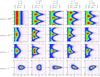 |
Fig. C.1 Probability density functions, f2D(p,ψ | p0,ψ0,Σp), with infinite S/N on intensity, computed for a given set of polarization parameters, namely ψ0 = 0° and p0 = 0.1 (dashed lines). Each row corresponds to a specific level of the S/N p0/σp,G = 0.01,0.5,1, and 5, from top to bottom. Various configurations of the covariance matrix are shown (in the different columns). Furthest left is the standard case: no ellipticity and no correlation. The next two columns show the impact of ellipticities ε = 1 / 2 and 2. The last two columns deal with correlations ρ = −1 / 2 and + 1 / 2. White crosses indicate the mean likelihood estimates of the PDF ( |

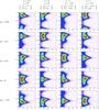 |
Fig. C.2 Probability density functions, f2D(p,ψ | p0,ψ0,Σp), plotted for various values of ψ0 (rows), spanning from − π/ 8 to 3π/ 8, and computed for four configurations of the covariance matrix (columns), parameterized by ε and ρ. The S/N on the intensity I is assumed to be infinite here. A true value of polarization p0 = 0.1 has been chosen, and with S/N p0/σp,G = 1. White crosses indicate the mean likelihood estimates of the PDF ( |
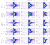 |
Fig. C.3 Probability density functions, f2D(p,ψ | I0,p0,ψ0,Σ), with finite S/N on intensity, I0/σI = 1, 2, and 5 (columns from left to right), computed for a given set of polarization parameters, ψ0 = 0° and p0 = 0.1 (dashed lines), and a S/N on the polarized intensity set to p0/σp,G = 1. Correlation coefficients ρQ and ρU are set to zero. Various configurations of the covariance matrix are shown (rows). White crosses indicate the mean likelihood estimates of the PDF ( |
Appendix D: General PDF of p and ψ
In the context of communication network science, Aalo et al. (2007) derived full expressions for the PDFs of envelope and phase quantities in the general case. These expressions can be directly translated to express the PDF of the polarization fraction and angle, p and ψ.
We can apply the rotation of the covariance introduced in Sect. 2.1 by an angle θ, given by Eq. (5), to remove the correlation term between the Stokes parameters. We define the mean and the variance of the normalized Stokes parameters in this new frame by  (D.1)and
  (D.2)The PDF of p is now written as
 ![Mathematical equation: \appendix \setcounter{section}{4} \begin{eqnarray} f_{p}(p\,|\,p_0,\psi_0,\tens{\Sigma}_{p}) & = &\frac{p}{2\sigma_1\sigma_2} \exp \left\{-\frac{1}{2}\left[\frac{\mu_1^2}{\sigma_1^2} + \frac{\mu_2^2}{\sigma_2^2} + \frac{p^2}{2} \left(\frac{1}{\sigma_1^2} + \frac{1}{\sigma_2^2} \right) \right] \right\} \nonumber \\ &&\quad \times \sum\limits_{n\,=\,0}^{\infty} \frac{ \zeta_n\mathcal{I}_n\left( \frac{p^2}{4}\left( \frac{1}{\sigma_2^2} - \frac{1}{\sigma_1^2} \right) \right)} {\left[\left(\frac{\mu_1}{\sigma_1^2}\right)^2 + \left( \frac{\mu_2}{\sigma_2^2}\right)^2 \right]^n} \scalebox{1.7}{\Bigg\{} \mathcal{I}_{2n} \left(p\sqrt{\left(\frac{\mu_1}{\sigma_1^2}\right)^2 +\left(\frac{\mu_2}{\sigma_2^2}\right)^2}\,\right) \sum\limits_{k\,=\,0}^{n}\delta_kC_k^n \left[\left( \frac{\mu_1}{\sigma_1^2}\right)^2\!-\left(\frac{\mu_2}{\sigma_2^2}\right)^2 \right]^{n-k} \left(2\frac{\mu_1\mu_2}{\sigma_1^2\sigma_2^2}\right)^k \scalebox{1.7}{\Bigg\}}, \end{eqnarray}](/articles/aa/full_html/2015/02/aa22271-13/aa22271-13-eq319.png) (D.3)with ℐn the nth-order modified Bessel function of the first kind. Here ζ0 = 1 and ζn = 2 for n ≠ 0,
(D.3)with ℐn the nth-order modified Bessel function of the first kind. Here ζ0 = 1 and ζn = 2 for n ≠ 0,  are binomial coefficients, and δk is defined by
  (D.4)It should be noted that the above expression converges so fast that only a few terms of the infinite sum are required to obtain sufficient accuracy. On the other hand, the PDF of the polarization angle is given by
 ![Mathematical equation: \appendix \setcounter{section}{4} \begin{eqnarray} f_{\psi}(\psi\,|\,p_0,\psi_0,\tens{\Sigma}_{p}) &=& \exp\left[-\frac{1}{1-\rho^2} \left(\frac{Q_0^2}{2\sigma_{ Q}^2} + \frac{U_0^2}{2\sigma_{ U}^2} - \frac{\rho Q_0 U_0}{\sigma_{ Q}\sigma_{ U}} \right) \right] \nonumber \\ &&\quad \times\,\frac{\sqrt{1-\rho^2}}{\pi\sigma_{ Q}\sigma_{ U}\mathcal{A}(\psi)} \left\{1 + \frac{\sqrt{\pi}\mathcal{B}(\psi)}{\sqrt{\mathcal{A}(\psi)}} \exp\left[ \frac{\mathcal{B}^2(\psi)}{\mathcal{A}(\psi)} \right] \mathrm{erfc} \left[ -\frac{\mathcal{B}(\psi)}{\sqrt{\mathcal{A}(\psi)}} \right] \right\}, \end{eqnarray}](/articles/aa/full_html/2015/02/aa22271-13/aa22271-13-eq328.png) (D.5)where
(D.5)where ![Mathematical equation: \appendix \setcounter{section}{4} \begin{eqnarray} \mathcal{A}(\psi) &=& \frac{2 \cos^2 2\psi}{\sigma_{ Q}^2} + \frac{2\sin^2 2\psi}{\sigma_{ U}^2} - 4\frac{\rho \sin 2\psi \cos 2\psi}{\sigma_{ Q}\sigma_{ U}}, \quad\quad\quad\\ \mathcal{B}(\psi) &=& \frac{1}{\sqrt{1-\rho^2}} \left[ \frac{\cos 2\psi}{\sigma_{ Q}} \left(\frac{Q_0}{\sigma_{ Q}} - \frac{\rho U_0}{\sigma_{ U}} \right) + \frac{\sin 2\psi}{\sigma_{ U}} \left( \frac{U_0}{\sigma_{ U}} - \frac{\rho Q_0}{\sigma_{ Q}} \right) \right],\quad\quad\quad \end{eqnarray}](/articles/aa/full_html/2015/02/aa22271-13/aa22271-13-eq329.png) and
and ![Mathematical equation: \appendix \setcounter{section}{4} \begin{equation} \mathrm{erfc}(z) = \frac{2}{\sqrt{\pi}} \int\limits_z^{\infty} \exp \left[-x^2\right] {\rm d}x \end{equation}](/articles/aa/full_html/2015/02/aa22271-13/aa22271-13-eq330.png) (D.8)is the complementary error function.
(D.8)is the complementary error function.
Appendix E: Impact of ρQ and ρU on ε and ρ
The covariance matrix Σ is positive definite, so may be written as a Cholesky product Σ = LTL, with  (E.1)The six Lij are independent, unlike the six parameters of the covariance matrix, (σI,σQ,σU,ρ,ρQ,ρU), or the parameters that we use in this paper, (σI,σQ,ε,ρ,ρQ,ρU). In the general case, these are given in terms of the Lij as (assuming I0 = 1)
  (E.2)When there is no correlation between I and the Q or U components, then L12 = L13 = 0, which leads to the following system:
 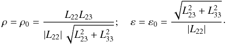 (E.3)The ellipticity and the correlation coefficient are therefore modified by the presence of the correlation between I and (Q,U). A little algebra leads to expressions for ε and ρ as functions of ε0, ρ0, ρQ, and ρU, namely
 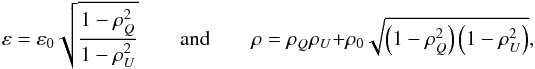 (E.4)which are Eqs. (26).
Appendix F: Derivation of conventional uncertainties
We describe here how the expressions for the conventional uncertainties of p and ψ, which were introduced in Sect. 4.3, are obtained from the derivatives of p and ψ. We first note that we generally have ![Mathematical equation: \appendix \setcounter{section}{6} \begin{equation} \sigma^{2}_{X}=E\Big[(X-E[X])^{2}\Big]=E\Big[({\rm d}X)^{2}\Big], \label{edx} \end{equation}](/articles/aa/full_html/2015/02/aa22271-13/aa22271-13-eq346.png) (F.1)where dX = X − E [ X ] is an infinitesimal element.
(F.1)where dX = X − E [ X ] is an infinitesimal element.
The conventional uncertainty of p can therefore be given by the expression ![Mathematical equation: \hbox{$\sigma^{2}_{{p},{\rm C}}\,{=}\,E\left[({\rm d}p)^{2}\right]$}](/articles/aa/full_html/2015/02/aa22271-13/aa22271-13-eq348.png) . Using the expression for p we obtain
. Using the expression for p we obtain 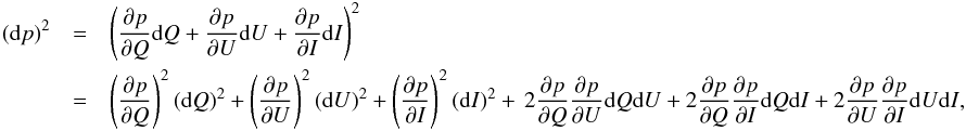 (F.2)where the partial derivatives are
  (F.3)This leads to the following expression for the conventional uncertainty:
 ![Mathematical equation: \appendix \setcounter{section}{6} \begin{eqnarray} \sigma^{2}_{p,{\rm C}} &=& \dfrac{1}{p^{2}I^{4}}\, E\Big[ Q^{2}({\rm d}Q)^{2}+U^{2}({\rm d}U)^{2}+p^{4}I^{2}({\rm d}I)^{2} +2QU{\rm d}Q{\rm d}U-2QIp^{2}{\rm d}Q{\rm d}I-2UIp^{2}{\rm d}U{\rm d}I \Big] \nonumber \\ &=& \dfrac{1}{p^{2}I^{4}}\Big( Q^{2}E\left[ (Q-E[Q])^{2}\right] + U^{2}E\left[ (U-E[U])^{2}\right] + p^{4}I^{2}E\left[ (I-E[I])^{2}\right] \nonumber \\ && \qquad + 2QUE\Big[ (Q-E[Q]) (U-E[U]) \Big] - 2QIp^{2}E\Big[ (Q-E[Q]) (I-E[I]) \Big] - 2UIp^{2}E\Big[ (U-E[U]) (I-E[I]) \Big] \Big). \end{eqnarray}](/articles/aa/full_html/2015/02/aa22271-13/aa22271-13-eq351.png) (F.4)This finally leads to
(F.4)This finally leads to  (F.5)Similarly we can derive an expression for the non-conventional uncertainty of the polarization angle, ψ, given by
 ![Mathematical equation: \hbox{$\sigma^{2}_{\psi,{\rm C}}\,{=}\,E\left[({\rm d}\psi)^{2}\right]$}](/articles/aa/full_html/2015/02/aa22271-13/aa22271-13-eq353.png) . Using the expression of ψ, we obtain the partial derivatives
. Using the expression of ψ, we obtain the partial derivatives 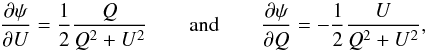 (F.6)as well as an expression for the conventional ψ uncertainty:
 ![Mathematical equation: \appendix \setcounter{section}{6} \begin{eqnarray} \sigma_{\psi,{\rm C}}^2 = E\left[\left(\dfrac{\partial\psi}{\partial U}{\rm d}U +\dfrac{\partial\psi}{\partial Q}{\rm d}Q\right)^2\right] = E \left[\left(\dfrac{Q{\rm d}U-U{\rm d}Q}{2p^{2}I^{2}}\right)^2\right] &=& E \left[ \dfrac{Q^{2}{\rm d}U^{2}+U^{2}{\rm d}Q^{2}-2QU{\rm d}Q{\rm d}U}{4p^{4}I^{4}}\right] \nonumber \\ \label{eq:sigpsi_cla_1} &=& \dfrac{Q^2\sigma_{ UU}+U^2\sigma_{ QQ} -2QU\sigma_{ QU}}{4p^{4}I^{4}}\cdot \end{eqnarray}](/articles/aa/full_html/2015/02/aa22271-13/aa22271-13-eq355.png) (F.7)Using Eq. (F.5) and assuming σII = σIQ = σIU = 0, we find
(F.7)Using Eq. (F.5) and assuming σII = σIQ = σIU = 0, we find 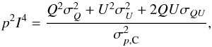 (F.8)and replacing this expression in Eq. (F.7) finally leads to
 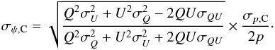 (F.9)The above two expressions for the conventional estimates have been obtained in the small-error limit, and therefore they are formally inapplicable to the large uncertainty regime. In Sect. 4 we discuss the extent to which they can provide reasonable proxies for the errors, even at low S/N.
Planck (http://www.cosmos.esa.int/web/planck) is a project of the European Space Agency (ESA) with instruments provided by two scientific consortia funded by ESA member states (in particular the lead countries France and Italy), with contributions from NASA (USA) and with telescope reflectors provided by a collaboration between ESA and a scientific consortium led and funded by Denmark.
Acknowledgments
This paper was developed to support the analysis of data from the Planck satellite. The development of Planck has been supported by: ESA; CNES and CNRS/INSU-IN2P3-INP (France); ASI, CNR, and INAF (Italy); NASA and DoE (USA); STFC and UKSA (UK); CSIC, MICINN, JA, and RES (Spain); Tekes, AoF, and CSC (Finland); DLR and MPG (Germany); CSA (Canada); DTU Space (Denmark); SER/SSO (Switzerland); RCN (Norway); SFI (Ireland); FCT/MCTES (Portugal); and PRACE (EU). A description of the Planck Collaboration and a list of its members, including the technical or scientific activities in which they have been involved, can be found at http://www.cosmos.esa.int/web/planck/planck-collaboration. We would also like to thank P. Leahy, S. Prunet, and D. Scott for their very useful comments.
References
- Aalo, V. A., Efthymoglou, G. P., & Chayawan, C. 2007, IEEE Comm. Lett., 11, 985 [CrossRef] [Google Scholar]
- Abramowitz, M., & Stegun, I. 1964, Handbook of Mathematical Functions (National Bureau of Standards) [Google Scholar]
- Benoît, A., Ade, P., Amblard, A., et al. 2004, A&A, 424, 571 [NASA ADS] [CrossRef] [EDP Sciences] [Google Scholar]
- Bernard, J.-P., Ade, P., De Bernardis, P., et al. 2007, in EAS Pub. Ser. 23, eds. M.-A. Miville-Deschênes, & F. Boulanger, 189 [Google Scholar]
- Boissier, J., Bockelée-Morvan, D., Biver, N., et al. 2009, Earth Moon Planets, 105, 89 [NASA ADS] [CrossRef] [Google Scholar]
- Clarke, D., Naghizadeh-Khouei, J., Simmons, J. F. L., & Stewart, B. G. 1993, A&A, 269, 617 [NASA ADS] [Google Scholar]
- Dotson, J. L., Vaillancourt, J. E., Kirby, L., et al. 2010, ApJS, 186, 406 [NASA ADS] [CrossRef] [Google Scholar]
- Dowell, C. D., Hildebrand, R. H., Schleuning, D. A., et al. 1998, ApJ, 504, 588 [NASA ADS] [CrossRef] [Google Scholar]
- Fissel, L. M., Ade, P. A. R., Angilè, F. E., et al. 2010, in SPIE Conf. Ser., 7741 [Google Scholar]
- Girart, J. M., Rao, R., & Marrone, D. P. 2006, Science, 313, 812 [NASA ADS] [CrossRef] [PubMed] [Google Scholar]
- Gradshteyn, I. S., & Ryzhik, I. M. 2007, Table of Integrals, Series, and Products (Elsevier) [Google Scholar]
- Greaves, J. S., Holland, W. S., Jenness, T., et al. 2003, MNRAS, 340, 353 [NASA ADS] [CrossRef] [Google Scholar]
- Jarosik, N., Bennett, C. L., Dunkley, J., et al. 2011, ApJS, 192, 14 [NASA ADS] [CrossRef] [Google Scholar]
- Li, H., Dowell, C. D., Kirby, L., Novak, G., & Vaillancourt, J. E. 2008, Appl. Opt., 47, 422 [NASA ADS] [CrossRef] [PubMed] [Google Scholar]
- Montier, L. A., Plaszczynski, S., Levrier, F., et al. 2015, A&A, 574, A136 [Google Scholar]
- Mood, A. M., & Graybill, A. F. 1974, Introduction to the Theory of Statistics, 3rd edn. (New-York: McGraw-Hill) [Google Scholar]
- Naghizadeh-Khouei, J., & Clarke, D. 1993, A&A, 274, 968 [NASA ADS] [Google Scholar]
- Page, L., Hinshaw, G., Komatsu, E., et al. 2007, ApJS, 170, 335 [NASA ADS] [CrossRef] [Google Scholar]
- Pérez-Sánchez, A. F., & Vlemmings, W. H. T. 2013, A&A, 551, A15 [NASA ADS] [CrossRef] [EDP Sciences] [Google Scholar]
- Planck Collaboration IntSPlanck Collaboration Int. XIX. 2014, A&A, submitted [arXiv:1405.0871] [Google Scholar]
- Platt, S. R., Hildebrand, R. H., Pernic, R. J., Davidson, J. A., & Novak, G. 1991, PASP, 103, 1193 [NASA ADS] [CrossRef] [Google Scholar]
- Quinn, J. L. 2012, A&A, 538, A65 [NASA ADS] [CrossRef] [EDP Sciences] [Google Scholar]
- Renbarger, T., Chuss, D. T., Dotson, J. L., et al. 2004, PASP, 116, 415 [NASA ADS] [CrossRef] [Google Scholar]
- Rice, S. O. 1945, Bell Systems Tech. J., 24, 46 [CrossRef] [Google Scholar]
- Schleuning, D. A., Dowell, C. D., Hildebrand, R. H., Platt, S. R., & Novak, G. 1997, PASP, 109, 307 [NASA ADS] [CrossRef] [Google Scholar]
- Serkowski, K. 1958, Acta Astron., 8, 135 [NASA ADS] [Google Scholar]
- Serkowski, K. 1962, Adv. Astron. Astrophys., 1, 290 [Google Scholar]
- Simmons, J. F. L., & Stewart, B. G. 1985, A&A, 142, 100 [NASA ADS] [Google Scholar]
- Tauber, J. A., Mandolesi, N., Puget, J., et al. 2010, A&A, 520, A1 [NASA ADS] [CrossRef] [EDP Sciences] [Google Scholar]
- Thum, C., Wiesemeyer, H., Paubert, G., Navarro, S., & Morris, D. 2008, PASP, 120, 777 [NASA ADS] [CrossRef] [Google Scholar]
- Vaillancourt, J. E. 2006, PASP, 118, 1340 [Google Scholar]
- Vaillancourt, J. E., & Matthews, B. C. 2012, ApJS, 201, 13 [NASA ADS] [CrossRef] [Google Scholar]
- Vinokur, M. 1965, Ann. Astrophys., 28, 412 [NASA ADS] [Google Scholar]
- Wardle, J. F. C., & Kronberg, P. P. 1974, ApJ, 194, 249 [NASA ADS] [CrossRef] [Google Scholar]
All Figures
|
Fig. 1 Illustrations of the noise distribution in the (Q, U) plane. The solid and dashed blue lines represent the 1σ probability contours around the true polarization values (Q0, U0), also parameterized by (p0, ψ0). Left: the canonical case (ε = 1, ρ = 0) is shown as a solid line. The dashed line shows the introduction of a correlation ρ = 0.5, leading to an effective ellipticity (εeff> 1) rotated by an angle θ. Right: same transformation, starting from the elliptical case (ε = 2, ρ = 0). |
| In the text | |
|
Fig. 2 Impact of the initial true polarization angle ψ0 and of varying effective ellipticity εeff on the relative polarization fraction bias Δp/σp,0 (top) and the relative polarization angle bias Δψ/σψ,0 (bottom). We assume no correlation here, so that θ = 0, and we set the S/N to p0/σp,G = 2. The canonical case (εeff = 1) is shown by the red line. |
| In the text | |
|
Fig. 3 Impact of the effective ellipticity εeff on the levels of bias. Top: Δp/σp,0 as a function of the effective ellipticity εeff, displayed for three levels of the S/N, p0/σp,G = 1, 2, and 5. The grey shaded regions indicate the whole extent of variability due to ψ0 and θ spanning the range − π/ 2 to π/ 2. Bottom: maximum | Δψ | /σψ,0 value for ψ0 and θ spanning the range − π/ 2 to π/ 2, plotted as a function of the effective ellipticity εeff, displayed for four levels of the S/N, p0/σp,G = 0.5, 1, 2, and 5. |
| In the text | |
|
Fig. 4 Polarization fraction bias, normalized to the true value p0, as a function of the S/N I0/σI, plotted for three values of the polarization S/N, p0/σp,G, and values of the effective ellipticity εeff covering the canonical (full line), low (dark grey shaded region), and extreme (light grey shaded region) regimes of the covariance matrix. The intensity correlation coefficients are set to ρQ = ρU = 0. We only consider the domain where (I0/σI) > (p0/σp,G). |
| In the text | |
|
Fig. 5 Same as Fig. 4, but showing the bias on the polarization fraction relative to the dispersion proxy |
| In the text | |
|
Fig. 6 Probability |
| In the text | |
|
Fig. 7 Same as Fig. 6, but for the polarization angle uncertainty estimators. Left: σψ,0. Right: conventional σψ,C. |
| In the text | |
|
Fig. 8 True polarization angle uncertainty, σψ,0, as a function of the S/N, p0/σp,G. The three regimes (canonical, low, and extreme) of the covariance matrix are explored (solid line, light, and dark grey shaded regions, respectively). |
| In the text | |
|
Fig. 9 Probability density function (PDF) of the measured S/N p/σp,G (where σp,G is the geometric estimate) as a function of the true S/N p0/σp,0, with no ellipticity and correlation in the covariance matrix Σp. The mean likelihood, |
| In the text | |
|
Fig. 10 Construction of 68% confidence intervals |
| In the text | |
|
Fig. C.1 Probability density functions, f2D(p,ψ | p0,ψ0,Σp), with infinite S/N on intensity, computed for a given set of polarization parameters, namely ψ0 = 0° and p0 = 0.1 (dashed lines). Each row corresponds to a specific level of the S/N p0/σp,G = 0.01,0.5,1, and 5, from top to bottom. Various configurations of the covariance matrix are shown (in the different columns). Furthest left is the standard case: no ellipticity and no correlation. The next two columns show the impact of ellipticities ε = 1 / 2 and 2. The last two columns deal with correlations ρ = −1 / 2 and + 1 / 2. White crosses indicate the mean likelihood estimates of the PDF ( |
| In the text | |
|
Fig. C.2 Probability density functions, f2D(p,ψ | p0,ψ0,Σp), plotted for various values of ψ0 (rows), spanning from − π/ 8 to 3π/ 8, and computed for four configurations of the covariance matrix (columns), parameterized by ε and ρ. The S/N on the intensity I is assumed to be infinite here. A true value of polarization p0 = 0.1 has been chosen, and with S/N p0/σp,G = 1. White crosses indicate the mean likelihood estimates of the PDF ( |
| In the text | |
|
Fig. C.3 Probability density functions, f2D(p,ψ | I0,p0,ψ0,Σ), with finite S/N on intensity, I0/σI = 1, 2, and 5 (columns from left to right), computed for a given set of polarization parameters, ψ0 = 0° and p0 = 0.1 (dashed lines), and a S/N on the polarized intensity set to p0/σp,G = 1. Correlation coefficients ρQ and ρU are set to zero. Various configurations of the covariance matrix are shown (rows). White crosses indicate the mean likelihood estimates of the PDF ( |
| In the text | |
Current usage metrics show cumulative count of Article Views (full-text article views including HTML views, PDF and ePub downloads, according to the available data) and Abstracts Views on Vision4Press platform.
Data correspond to usage on the plateform after 2015. The current usage metrics is available 48-96 hours after online publication and is updated daily on week days.
Initial download of the metrics may take a while.