| Issue |
A&A
Volume 574, February 2015
|
|
|---|---|---|
| Article Number | A135 | |
| Number of page(s) | 17 | |
| Section | Astrophysical processes | |
| DOI | https://doi.org/10.1051/0004-6361/201322271 | |
| Published online | 10 February 2015 | |
Online material
Appendix A: Expressions for PDFs
Here we present expressions for the 2D PDFs that are discussed in Sect. 2:


where we have defined the functions 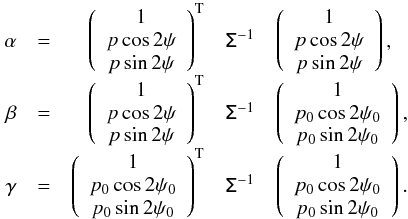 (A.5)
(A.5)
Appendix B: Computation of f2D
The 3D PDF of (I,p,ψ) is given by ![]() (B.1)To compute the 2D PDF of (p,ψ), we marginalize over total intensity. However, some care is required here, because the above expression for f(I,p,ψ) is only valid for
(B.1)To compute the 2D PDF of (p,ψ), we marginalize over total intensity. However, some care is required here, because the above expression for f(I,p,ψ) is only valid for ![]() (i.e., we cannot measure negative p unless I happens to be negative owing to noise) and f must be taken to be zero otherwise. This means that the marginalization is performed over
(i.e., we cannot measure negative p unless I happens to be negative owing to noise) and f must be taken to be zero otherwise. This means that the marginalization is performed over ![]() for positive p and over
for positive p and over ![]() for negative p:
for negative p: 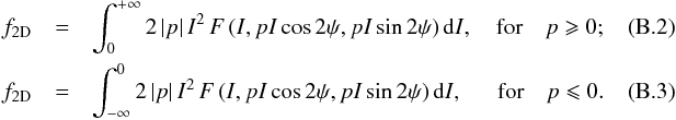 The integrand may be written so as to exhibit the dependence on total intensity,
  (B.4)and then we make use of the functions (Gradshteyn & Ryzhik 2007):
 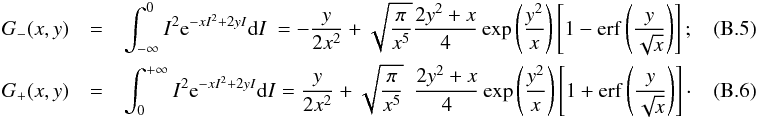 Elementary replacement of (x,y) by (α/ 2,I0β/ 2) yields the PDF of Eqs. (A.2) and (A.3).
Appendix C: Illustrations of f2D
We illustrate the shape of the 2D PDF f2D(p,ψ | I0,p0,ψ0,Σ) in Fig. C.1, for the case of a perfectly known intensity having no correlation with the polarization. Starting from a given couple of true polarization parameters, ψ0 = 0° and p0 = 0.1, the PDF is computed for various S/Ns, p0/σp,G, and settings of the covariance matrix. The S/N p0/σp,G is varied from 0.01 to 0.5, 1, and 5 (top to bottom). The dashed crossing lines show the location of the initial true polarization values. The leftmost column shows the results obtained when the covariance matrix is assumed to be diagonal and symmetric, (i.e., ε = 1 and ρ = 0), as was usually done in previous works on polarization data. The distribution along the ψ axis is fully symmetric around 0, implying the absence of bias on the polarization angle. When varying the ellipticity ε from 1/2 to 2 (Cols. 2 and 3), we still observe symmetrical PDFs in this configuration, but multiple peaks appear at low S/N. In the presence of correlation, i.e., ρ = −1 / 2 and 1 / 2 (Cols. 4 and 5), the maximum peak is now slightly shifted in p and ψ, with an asymmetric PDF around the initial ψ0 value.
In the usual canonical case, ε = 1 and ρ = 0, the PDF remains strictly symmetric regardless of the value of the initial true polarization angle ψ0. However, when changing the true polarization angle ψ0, as shown in Fig. C.2, the PDF may become asymmetrical once the ellipticity ε ≠ 1 or the correlation ρ ≠ 0. This will induce a statistical bias in the measurement of the polarization angle ψ, which could be positive or negative depending on the covariance matrix and the true value ψ0, as discussed in Sect. 3.
Examples of 2D PDFs f2D(p,ψ | I0,p0,ψ0,Σ) for finite values of I0/σI (1, 2, and 5), and various ε and ρ situations, are shown in Fig. C.3 for the case ρQ = ρU = 0. The true polarization parameters are p0 = 0.1 and ψ0 = 0°, and the polarization S/N is set to p0/σp,G = 1, so these plots may be directly compared to the third row of Fig. C.1. The effect of varying I0/σI on the overall shape of the PDF seems rather small, but the position of the maximum likelihood in (p,ψ) is noticeably changed to lower values of p when I0/σI ≲ 2, while the mean likelihood appears to be increased.
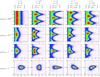 |
Fig. C.1
Probability density functions, f2D(p,ψ | p0,ψ0,Σp), with infinite S/N on intensity, computed for a given set of polarization parameters, namely ψ0 = 0° and p0 = 0.1 (dashed lines). Each row corresponds to a specific level of the S/N p0/σp,G = 0.01,0.5,1, and 5, from top to bottom. Various configurations of the covariance matrix are shown (in the different columns). Furthest left is the standard case: no ellipticity and no correlation. The next two columns show the impact of ellipticities ε = 1 / 2 and 2. The last two columns deal with correlations ρ = −1 / 2 and + 1 / 2. White crosses indicate the mean likelihood estimates of the PDF ( |
| Open with DEXTER | |
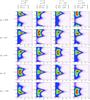 |
Fig. C.2
Probability density functions, f2D(p,ψ | p0,ψ0,Σp), plotted for various values of ψ0 (rows), spanning from − π/ 8 to 3π/ 8, and computed for four configurations of the covariance matrix (columns), parameterized by ε and ρ. The S/N on the intensity I is assumed to be infinite here. A true value of polarization p0 = 0.1 has been chosen, and with S/N p0/σp,G = 1. White crosses indicate the mean likelihood estimates of the PDF ( |
| Open with DEXTER | |
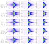 |
Fig. C.3
Probability density functions, f2D(p,ψ | I0,p0,ψ0,Σ), with finite S/N on intensity, I0/σI = 1, 2, and 5 (columns from left to right), computed for a given set of polarization parameters, ψ0 = 0° and p0 = 0.1 (dashed lines), and a S/N on the polarized intensity set to p0/σp,G = 1. Correlation coefficients ρQ and ρU are set to zero. Various configurations of the covariance matrix are shown (rows). White crosses indicate the mean likelihood estimates of the PDF ( |
| Open with DEXTER | |
Appendix D: General PDF of p and ψ
In the context of communication network science, Aalo et al. (2007) derived full expressions for the PDFs of envelope and phase quantities in the general case. These expressions can be directly translated to express the PDF of the polarization fraction and angle, p and ψ.
We can apply the rotation of the covariance introduced in Sect. 2.1 by an angle θ, given by Eq. (5), to remove the correlation term between the Stokes parameters. We define the mean and the variance of the normalized Stokes parameters in this new frame by ![]() (D.1)and
(D.1)and ![]() (D.2)The PDF of p is now written as
(D.2)The PDF of p is now written as 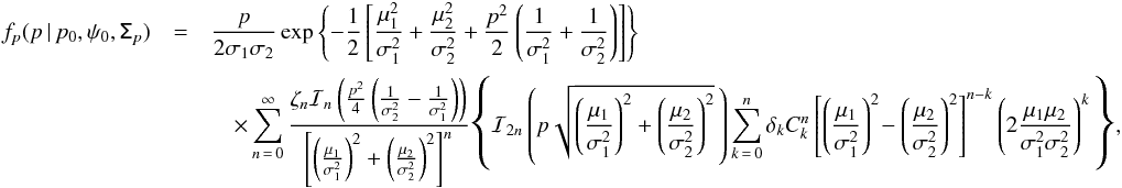 (D.3)with ℐn the nth-order modified Bessel function of the first kind. Here ζ0 = 1 and ζn = 2 for n ≠ 0,
 ![]() are binomial coefficients, and δk is defined by
are binomial coefficients, and δk is defined by 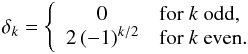 (D.4)It should be noted that the above expression converges so fast that only a few terms of the infinite sum are required to obtain sufficient accuracy. On the other hand, the PDF of the polarization angle is given by
 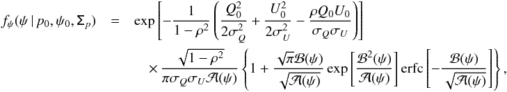 (D.5)where
 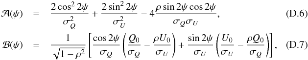 and
and 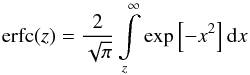 (D.8)is the complementary error function.
Appendix E: Impact of ρQ and ρU on ε and ρ
The covariance matrix Σ is positive definite, so may be written as a Cholesky product Σ = LTL, with 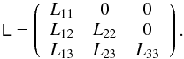 (E.1)The six Lij are independent, unlike the six parameters of the covariance matrix, (σI,σQ,σU,ρ,ρQ,ρU), or the parameters that we use in this paper, (σI,σQ,ε,ρ,ρQ,ρU). In the general case, these are given in terms of the Lij as (assuming I0 = 1)
 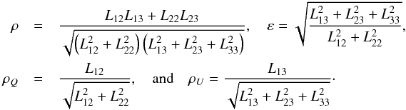 (E.2)When there is no correlation between I and the Q or U components, then L12 = L13 = 0, which leads to the following system:
  (E.3)The ellipticity and the correlation coefficient are therefore modified by the presence of the correlation between I and (Q,U). A little algebra leads to expressions for ε and ρ as functions of ε0, ρ0, ρQ, and ρU, namely
 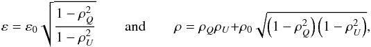 (E.4)which are Eqs. (26).
Appendix F: Derivation of conventional uncertainties
We describe here how the expressions for the conventional uncertainties of p and ψ, which were introduced in Sect. 4.3, are obtained from the derivatives of p and ψ. We first note that we generally have ![]() (F.1)where dX = X − E [ X ] is an infinitesimal element.
(F.1)where dX = X − E [ X ] is an infinitesimal element.
The conventional uncertainty of p can therefore be given by the expression ![]() . Using the expression for p we obtain
. Using the expression for p we obtain 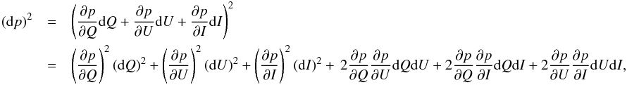 (F.2)where the partial derivatives are
  (F.3)This leads to the following expression for the conventional uncertainty:
 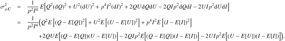 (F.4)This finally leads to
  (F.5)Similarly we can derive an expression for the non-conventional uncertainty of the polarization angle, ψ, given by
 ![]() . Using the expression of ψ, we obtain the partial derivatives
. Using the expression of ψ, we obtain the partial derivatives 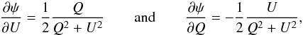 (F.6)as well as an expression for the conventional ψ uncertainty:
 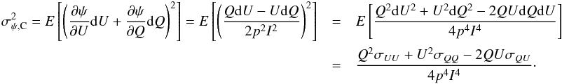 (F.7)Using Eq. (F.5) and assuming σII = σIQ = σIU = 0, we find
 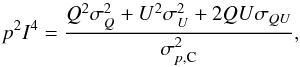 (F.8)and replacing this expression in Eq. (F.7) finally leads to
 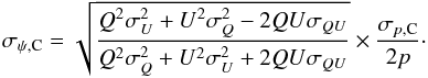 (F.9)The above two expressions for the conventional estimates have been obtained in the small-error limit, and therefore they are formally inapplicable to the large uncertainty regime. In Sect. 4 we discuss the extent to which they can provide reasonable proxies for the errors, even at low S/N.
© ESO, 2015
Current usage metrics show cumulative count of Article Views (full-text article views including HTML views, PDF and ePub downloads, according to the available data) and Abstracts Views on Vision4Press platform.
Data correspond to usage on the plateform after 2015. The current usage metrics is available 48-96 hours after online publication and is updated daily on week days.
Initial download of the metrics may take a while.