| Issue |
A&A
Volume 595, November 2016
|
|
|---|---|---|
| Article Number | A57 | |
| Number of page(s) | 12 | |
| Section | Astronomical instrumentation | |
| DOI | https://doi.org/10.1051/0004-6361/201628809 | |
| Published online | 28 October 2016 | |
Polarization measurement analysis
III. Analysis of the polarization angle dispersion function with high precision polarization data
1 Department of Physics, School of Science and Technology, Nazarbayev University, 010000 Astana, Kazakhstan
e-mail: This email address is being protected from spambots. You need JavaScript enabled to view it.
2 Université de Toulouse, UPS-OMP, IRAP, 31028 Toulouse Cedex 4, France
3 CNRS, IRAP, 9 Av. colonel Roche, BP 44346, 31028 Toulouse Cedex 4, France
4 LERMA/LRA − ENS Paris et Observatoire de Paris, 24 rue Lhomond, 75231 Paris Cedex 05, France
Received: 28 April 2016
Accepted: 4 August 2016
Abstract
High precision polarization measurements, such as those from the Planck satellite, open new opportunities for the study of the magnetic field structure as traced by polarimetric measurements of the interstellar dust emission. The polarization parameters suffer from bias in the presence of measurement noise. It is critical to take into account all the information available in the data in order to accurately derive these parameters. In our previous work, we studied the bias on polarization fraction and angle, various estimators of these quantities, and their associated uncertainties. The goal of this paper is to characterize the bias on the polarization angle dispersion function that is used to study the spatial coherence of the polarization angle. We characterize for the first time the bias on the conventional estimator of the polarization angle dispersion function and show that it can be positive or negative depending on the true value. Monte Carlo simulations were performed to explore the impact of the noise properties of the polarization data, as well as the impact of the distribution of the true polarization angles on the bias. We show that in the case where the ellipticity of the noise in (Q,U) varies by less than 10%, one can use simplified, diagonal approximation of the noise covariance matrix. In other cases, the shape of the noise covariance matrix should be taken into account in the estimation of the polarization angle dispersion function. We also study new estimators such as the dichotomic and the polynomial estimators. Though the dichotomic estimator cannot be directly used to estimate the polarization angle dispersion function, we show that, on the one hand, it can serve as an indicator of the accuracy of the conventional estimator and, on the other hand, it can be used for deriving the polynomial estimator. We propose a method for determining the upper limit of the bias on the conventional estimator of the polarization angle dispersion function. The method is applicable to any linear polarization data set for which the noise covariance matrices are known.
Key words: polarization / methods: statistical / methods: data analysis / techniques: polarimetric
© ESO, 2016
1. Introduction
The linear polarization of the incoming radiation can be described by the Stokes parameters Q and U along with the total intensity I. The polarization fraction p and the polarization angle ψ are derived from I, Q and U, and bias on these parameters appears in the presence of measurement noise (Serkowski 1958; Wardle & Kronberg 1974; Simmons & Stewart 1985; Vaillancourt 2006; Quinn 2012). This issue has recently been addressed by Montier et al. (2015a,b), hereafter Papers I and II of this series on the polarization measurement analysis of high precision data. In this work, which we refer to as Paper III, we aim to characterize the bias on the polarization angle dispersion function − a polarization parameter that measures the spatial coherence of the polarization angle.
The interstellar magnetic field structure can be revealed by the polarimetric measurements of synchrotron radiation and of dust thermal emission and extinction (Mathewson & Ford 1970; Han 2002; Beck & Gaensler 2004; Heiles & Troland 2005; Fletcher 2010). The interstellar dust particles are aligned with respect to the magnetic field (Hall & Mikesell 1949; Hiltner 1949; Lazarian & Hoang 2008). This leads to linear polarization in the visible, infrared and submillimetre (Benoît et al. 2004; Vaillancourt 2007; Andersson et al. 2015). The interstellar dust polarization yields information about the direction of the plane of the sky (POS) component of the magnetic field. Heiles (1996) have used observations of polarization by dust extinction and found that the inclination of the Galactic magnetic field with respect to the plane of the disk of matter is about 7°. Recently Planck Collaboration Int. XIX (2015) have derived the all-sky magnetic field direction map as projected onto the POS from the Planck Satellite data. They have also used the polarization angle dispersion function and have studied its correlation with the polarization fraction. In the framework of their analysis, the observed anti-correlation allows to come to a conclusion that the observed polarization at large scales (diffuse ISM, large molecular clouds) largely depends on the magnetic field structure. Polarimetric measurement of the emission from molecular clouds and star forming regions help to better understand the role of the magnetic field in star formation (Matthews et al. 2009; Dotson et al. 2010; Tang et al. 2012; Zhang et al. 2010; Cortes et al. 2016).
Davis & Greenstein (1951) and Chandrasekhar & Fermi (1953) have calculated the angular dispersion in polarimetric measurements of distant stars (Hiltner 1951) to derive the strength of the magnetic field in the local spiral arm. Since then, the so-called Davis-Chandrasekhar-Fermi method has been widely used to derive some properties of the magnetic field such as the strength of its POS component (Lai et al. 2001; Sandstrom et al. 2002; Crutcher et al. 2004; Girart et al. 2006; Falceta-Gonçalves et al. 2008). In fact, this method is based on the polarization angle structure function, which is obtained as the average of the polarization angle dispersion function over the positions. The polarization angle structure function is also used to study the magnetic field direction that can be inferred from different types of polarimetric measurements. For example, Mao et al. (2010) computes the polarization angle structure function in order to study the structures traced by the synchrotron Faraday rotation measures.
Serkowski (1958) have shown that the structure function of the Stokes parameters Q and U reaches a limit. When the area, considered to calculate the structure function, becomes too large and includes non-connected regions, the parameters become spatially decorrelated. Poidevin et al. (2010) reports a similar behavior of the polarization angle structure function. The randomness of angles can be due not only to the physical decorrelation in the underlying pattern, but also to the noise of the measurement. According to Hildebrand et al. (2009), the polarization angle structure function contains contributions of the large-scale and turbulent magnetic field components. They have developed a method to estimate the strength of these components using the polarization angle structure function. The method has successfully been applied to polarimetry and interferometry data to characterize the magnetic turbulence power spectrum and magnetic field strength in molecular clouds (Houde et al. 2011a,b, 2016). The authors claim that its uncertainty can simply be calculated through the uncertainties of the angles used in the determination of the polarization angle structure function.
We have shown in Papers I and II that in order to accurately estimate the polarization fraction and polarization angle, one should take into account the full noise covariance matrix if possible. In this work, we study the behavior of the bias on the polarization angle dispersion function knowing the full noise covariance matrix and the distribution of the true polarization angles. We introduce new estimators of the polarization angle dispersion function and describe a method to evaluate an upper limit for the bias of the conventional estimator.
In Sect. 2 we introduce the notations and give the definition of the conventional estimator of the polarization angle dispersion function in terms of the Stokes parameters. In Sect. 3 we demonstrate the peculiarity of the bias. We also discuss the impact on the bias of the noise covariance matrix and of the distribution of the true polarization angles in the vicinity of the point of interest. We address the reliability of the conventional uncertainty on polarization angle dispersion function as well. In Sect. 4 we introduce alternative estimators and propose a method to evaluate the maximum bias of the conventional estimator for a given set of data.
2. Conventional estimator of the polarization angle dispersion function
2.1. Definition and notations
A POS component of polarized radiation is characterized by the true, that is, not affected by the measurement noise, polarization fraction  (1)and polarization orientation angle
  (2)where I0,Q0,U0 are the true Stokes parameters that describe the intensity and the linear polarization of the incoming radiation. Function arctan takes two arguments in order to choose the correct quadrant when calculating the arctangent of the ratio U/Q.
The true polarization angle dispersion function at the position x, where x is the 2D coordinate in the POS, is defined as the root mean square over the N(l) pairs of angles located within an area of radius l around x (see Fig. 1 for illustration): ![Mathematical equation: \begin{equation} \dpsiz (\vec{x},l) = \sqrt{ \frac{1}{N(l)} \sum_{i=1}^{N(l)} \left[\angz(\vec{x}) - \angz (\vec{x}+\vec{l}_i ) \right]^2 }. \label{eq:dpsiz} \end{equation}](/articles/aa/full_html/2016/11/aa28809-16/aa28809-16-eq18.png) (3)
(3) takes values between 0 and π/ 2. We note that it is also possible to consider only the angles contained in an annulus of a certain radius and width. In that case
  , where δ is the width of the annulus and l is the lag.
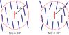 |
Fig. 1 Schematic view of the simulated configuration of polarization orientations. The polarization angle dispersion function is calculated at the position of the red line segment within the red-dotted circle of radius l. Left: uniform configuration. Right: random configuration. Both cases give |

When using the measured quantities, we will call this estimator the “conventional estimator” and denote it by  :
: ![Mathematical equation: \begin{equation} \cl (\vec{x},l) = \sqrt{ \frac{1}{N(l)} \sum_{i=1}^{N(l)} \left[\ang(\vec{x}) - \ang (\vec{x}+\vec{l}_i ) \right]^2 }. \label{eq:dpsi} \end{equation}](/articles/aa/full_html/2016/11/aa28809-16/aa28809-16-eq27.png) (4)The above formula takes the following form in terms of the Stokes Q and U parameters:
(4)The above formula takes the following form in terms of the Stokes Q and U parameters: ![Mathematical equation: \begin{eqnarray} \dpsi (\vec{x},l) &=& \left[\frac{1}{N(l)}\sum_{i=1}^{N(l)} \left(\dfrac{1}{2} \arctan \lbrack U(\mx)Q(\mxl)-Q(\mx)U(\mxl),\phantom{\sum_{i=1}}\right. \right. \nonumber\\ &&\left.\left.\phantom{\sum_{i=1}^{N(l)}}Q(\mx)Q(\mxl)+U(\mx)U(\mxl) \rbrack \right)^{2} \right]^{1/2}. \label{eq:dpsi_QU} \end{eqnarray}](/articles/aa/full_html/2016/11/aa28809-16/aa28809-16-eq28.png) (5)This equation is applicable to both and .
(5)This equation is applicable to both and .
Noise on any polarimetric measurement is characterized by a noise covariance matrix Σ. The noise covariance matrix of a linear polarization measurement has the following form: ![Mathematical equation: \begin{equation} \Sigma \equiv \left(\begin{array}{ccc} \sigma^2_{\it I} & \sigma_{\it IQ} & \sigma_{\it IU} \\[1mm] \sigma_{\it IQ} & \sigma^2_{\it Q} & \sigma_{\it QU} \\[1mm] \sigma_{\it IU} & \sigma_{\it QU} & \sigma^2_{\it U} \\ \end{array}\right), \label{eq:sigma} \end{equation}](/articles/aa/full_html/2016/11/aa28809-16/aa28809-16-eq30.png) (6)where
(6)where  (X = I,Q,U) characterizes the noise level in the X parameter (i.e., variance), and σXY (Y = I,Q,U) characterizes the correlation between noise on X and Y (i.e., covariance).
As we are interested only in the angle measurements, the intensity is assumed to be known exactly, so that the noise covariance matrix can be reduced to: ![Mathematical equation: \begin{equation} \Sigma_p = \left(\begin{array}{cc} \sigma^2_{\it Q} & \sigma_{\it QU} \\[0.5mm] \sigma_{\it QU} & \sigma^2_{\it U} \\ \end{array}\right). \label{eq:sigma_simple_zero} \end{equation}](/articles/aa/full_html/2016/11/aa28809-16/aa28809-16-eq37.png) (7)It is possible to fully characterize Σp using only two parameters (Montier et al. 2015a):
(7)It is possible to fully characterize Σp using only two parameters (Montier et al. 2015a): 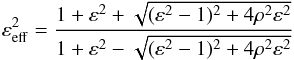 (8)and
  (9)Here ε and ρ are the ellipticity and correlation between noises on Q and U:
  (10)The reduced noise covariance matrix then takes the following form:
 ![Mathematical equation: \begin{equation} \Sigma_p = \frac{\sigma^2_p}{\sqrt{1-\rho^2}} \left(\begin{array}{cc} 1/ \varepsilon & \rho \\[0.5mm] \rho & \varepsilon \\ \end{array}\right), \label{eq:sigma_simple} \end{equation}](/articles/aa/full_html/2016/11/aa28809-16/aa28809-16-eq44.png) (11)where σp is a global polarization noise scaling factor, such that
(11)where σp is a global polarization noise scaling factor, such that  (Montier et al. 2015a).
The effective ellipticity εeff and the angle θ give the shape of the noise distribution in linear polarization, independently of the reference frame to which Q and U are attached.
In order to characterize the form of the noise covariance matrix, 3 regimes of εeff are considered in this study:
-
the canonical case:εeff = 1. This corresponds to the equality and independence between noise levels on Q and U:
 , σUQ = σUQ = 0;
 -
the low regime: 1 ≤ εeff< 1.1. This means that the differences and/or correlations between noise levels on Q and U are small;
-
the extreme regime: 1.1 ≤ εeff< 2. This means that the differences and/or correlations between noise levels on Q and U are large.
2.2. Monte Carlo simulations
In order to characterize the bias on the polarization angle dispersion function, we perform Monte Carlo (MC) simulations. We build numerical distribution functions (DFs) of using the following set of basic assumptions:
-
1.
We consider 10 pixels: 1 central pixel and 9 adjacent pixels to be contained within a circle of radius l, as shown in Fig. 1. In a regularly-gridded map there are 8 adjacent pixels, but a small difference (by 1 or 2) in the number of pixels does not affect the results of our simulations.
-
2.
All pixels have the same true polarization fraction p0 = 0.1 and the same noise covariance matrix Σp. The latter assumption seems to be reasonable because
 is usually calculated inside small areas, where the instrumental noise does not change much.
 -
3.
We perform NMC = 106 noise realizations at each run (i.e., for each simulated configuration, including the signal-to-noise ratio (S/N), the true value, the shape of the noise covariance matrix and the true polarization angles).
-
4.
We consider Gaussian noise on Q and U with a noise covariance matrix Σp.
-
5.
We vary the S/N of p between 0.1 and 30. We set σp = p0/ (S/N) to be used in Eq. (11).
-
6.
We vary ρ in the range [− 0.5, 0.5] and ϵ in the range [0.5, 2]. The low regime is obtained when using ρ ≃ 0 and ε ≃ 1; other cases (with ϵ ≤ 0.9, and ϵ ≥ 1.1 and ρ ≥ | 0.05 |) give the extreme regime of εeff.
We use ψ0,i to denote the true polarization angle for pixel i, and consider two cases of the configuration: the “uniform” and the “random” configurations. In the uniform configuration, all angles ψ0,i are the same for i ∈ [1,9], while ψ0,0 is calculated as:  (12)In the random configuration ψ0,i for i ∈ [1,9] are generated randomly and ψ0,0 is selected from a series of random values to obtain with (10-5)° precision using Equation 3 at each run. Examples of both configurations, uniform and random, are illustrated on left and right panels in Fig. 1, respectively. There are 10 representative sets of the true angles for each configuration and the true polarization angle dispersion function. They are obtained by varying ψ0,0 from 0 to π/ 2 with 10° (π/ 18) step for the uniform configuration and by generating additional sets for the random configuration.
Once ψ0,0 and ψ0,i are obtained, the following transformation is performed in order to get the corresponding Q and U parameters: ![Mathematical equation: \begin{eqnarray} Q_{0,i} &=& p_0 \, I_0 \, \cos(2\ang_{0,i}) , \ i \in[0,9], \\ U_{0,i} & =& p_0 \, I_0 \, \sin(2\ang_{0,i}), \ i \in[0,9], \label{eq:ppsi2qu} \end{eqnarray}](/articles/aa/full_html/2016/11/aa28809-16/aa28809-16-eq83.png) with I0 = 1. Random Gaussian noise is generated for each pixel for Q and U according to the noise covariance matrix and is added to the true values to obtain the simulated Stokes parameters for each pixel. The simulated measured polarization angle dispersion function is calculated using Eq. (5).
with I0 = 1. Random Gaussian noise is generated for each pixel for Q and U according to the noise covariance matrix and is added to the true values to obtain the simulated Stokes parameters for each pixel. The simulated measured polarization angle dispersion function is calculated using Eq. (5).
Once we have the simulated sample of 106 values of for the given , the configuration of the true angles and the noise level, we can build numerical DFs, which we denote as  . The shape of the DF for the given noise levels in the canonical case of the noise covariance matrix and in the uniform configuration of the true angles is illustrated in Fig. 2. At very low S/Ns, the distribution function peaks at
  , regardless of . The value
  (≃51.96°) corresponds to the result of with purely random distribution of angles. In fact, for a pair of angles in the range [− π/ 2,π/ 2], their absolute difference is distributed uniformly in the range [0,π/ 2]. The root mean square of this distribution gives .
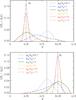 |
Fig. 2 Examples of the simulated distribution functions of the conventional estimator of the dispersion function |
3. Bias analysis
In the following, the bias on was calculated as follows:  (15)where
  is a realization of the conventional estimator of . We study different origins of the bias on by comparing the contributions of the biases due to the following parameters that affect its estimation: the true value (
 ), the shape of the noise covariance matrix (
 ), the distribution of the true angles (
 ) and the joint impact of these parameters (
 ).
).
3.1. Impact of the true value 
We calculated the average statistical bias induced by noise and the true value,  , in the case with εeff = 1 and uniform configuration of the true angles. Figure 3 represents (in colored plain curves) as a function of S/N, for values of ranging from 0 to π/ 2 in steps of π/ 16 (11.25°). If the S/N is high, corresponds to , whereas if S/N is low, does not represent . The closer to the bounds (0 or π/ 2), the larger the bias , even at high S/N (p0/σp> 10). The largest bias occurs in the case where
  , which is the most remote value from (where is the result for if the orientation angles are random). Also, the conventional estimator can be ambiguous if it gives results close to .
In the presence of noise, is biased, though not necessarily positively biased, whereas the polarization fraction p is always positively biased (Montier et al. 2015a). For a true value of lower than , the measured is positively biased, while it has negative bias for larger than .
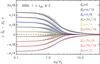 |
Fig. 3 Average bias on 106 MC noise realizations for the conventional estimator |
3.2. Impact of the (Q,U) effective ellipticity
Montier et al. (2015a) showed that the shape of the noise covariance matrix associated with a polarization measurement affects the bias on the polarization fraction p and angle ψ. Here we study the impact of the shape of the noise covariance matrix on the bias of the conventional estimator of the polarization angle dispersion function and evaluate under what conditions the assumption of non-correlated noise (i.e., εeff = 1) can be justified. For this purpose, we run the MC simulations as described in Sect. 2.2 in the three cases of the effective ellipticity and in the uniform configuration of the true angles.
We show in Fig. 3 the statistical bias of depending both on the true value and on the shape of the noise covariance matrix,  , as a function of S/N and for different true values . In the low regime the shape of Σp has practically no effect on the bias: the corresponding dispersion can not be seen in the figure as it coincides with the canonical case curves. A dispersion in the initial bias (corresonding to the amplitude of the gray areas) appears if there are important asymmetries in the shape of Σp, that is, in the extreme regime. We note that these asymmetries may either increase or decrease the statistical bias:
  in the gray areas are higher or lower than the colored curves, that is, closer to or farther from the “zero bias” line, that occurs for in the canonical case and shown by the dashed line in the figure. If the true polarization angle dispersion function is close to , that is, close to the zero bias line,
  is significant with respect to (for
  ). If is very different from , that is, remote from the zero bias line, both and become comparable for S/N ≥ 3 (for
  ).
).
The dispersion in the bias reaches its maximum at intermediate S/N (p0/σp ∈ [1,3]). At low S/N (p0/σp< 0.5), there is almost no impact of the shape of the noise covariance matrix on the bias and we observe only the bias due to : the dispersion of is much smaller than the level of . When the noise level is too high, it dominates any other effect. At high S/N, the noise level is low, so the estimation becomes accurate enough to become independent of the shape of the noise covariance matrix. Figure 4 shows the maximum absolute deviation of from over all possible values of as a function of εeff. The maximum deviation increases progressively with εeff and is the largest at p0/σp = 2 with  (π/ 34).
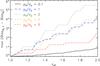 |
Fig. 4 Maximum absolute deviation of the bias induced by variations of the effective ellipticity between noise in (Q, U) and the true value |

Thus, the shape of the noise covariance matrix can significantly impact the bias on the polarization angle dispersion function. In the extreme regime and intermediate S/N, for the true values close to , the bias induced by the ellipticity and/or correlation between noise levels on Q and U is of the same order as the bias due to in the canonical case (as for the values of between 3π/ 16 to 3π/ 8 in Fig. 3): the width of the gray areas is comparable to the amplitude of the colored curves. Nevertheless, in the case where irregularities of the noise covariance matrix depart by less than 10% from the canonical case, that is, in the low regime, the impact of the asymmetry in the shape of the noise covariance matrix on the bias of is negligible (the amplitude of the deviation from the bias in the canonical case is very low and is not represented in the figure).
3.3. Impact of the true angles distribution
A multitude of different combinations of the true polarization angles ψ0,i can yield the same value . We study to which extent the polarization angle dispersion function can be affected by the configuration of the true angles. We compare the bias induced by the different configurations of the angles  to the bias due to the true value in the uniform configuration (seen in Sect. 3.1). For this purpose, we performed simulations in the canonical case of the noise covariance matrix for the 10 simulated combinations of the true polarization angles in each of the configurations (random and uniform). Figure 5 shows the dispersion σΔψ of the differences between angles of the central pixel and of the neighbor pixels Δψ0,i for i ∈ [1,9] as a function of in the canonical case of the noise covariance matrix and the random configuration of the true angles. The dispersion of the angles that give the value
  is also shown (the point between
  and
and  ). We would like to point out that, by construction, random distributions of the true angles that give
  and
and  do not exist. Also, the closer to these values (0 and π/ 2), the smaller the dispersion because there are less possible combinations of Δψ0,i.
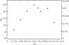 |
Fig. 5 Standard deviation of the difference between the true angle ψ0,0 and the true angles ψ0,i,i ∈ [1,9] as a function of the true polarization angle dispersion function |
In Fig. 6 we show the examples of the statistical bias  obtained in both configurations of the true angles. The different realizations of the uniform configuration in the canonical regime does not bring any contribution to the bias obtained in the canonical case of the noise covariance matrix and fully reproduce the colored curves of Fig. 3. But when the distribution of the angles deviates from uniformity and becomes random, variations in the bias appear. In fact, each pair of angles (ψ0,0,ψ0,i) has its proper Δψ0,i = ψ0,0−ψ0,i and only their mean squared sum gives . In the presence of noise,
  becomes biased. The sum of the biased quantities results in the dispersion of the total bias on .
Similarly to the case of the bias induced by both the true value and the shape of the noise covariance matrix , the dispersion in the bias due to the true value and the true angles distribution increases at intermediate S/N and diminishes at low and high S/N, for the same reason discussed in Sect. 3.2 (gray areas become larger at intermediate S/N in Fig. 6).  opens the widest range of possible Δψ0,i, ensuring the largest dispersion of values (Fig. 5). Thankfully, this value has a small bias due to : the corresponding colored curve in Fig. 6 is close to the zero bias level even at low S/N. At p0/σp = 2, the maximum dispersion of the bias for is almost 4° (≃π/ 45, corresponding to the width of the grey area) when the angles are distributed randomly, whereas the bias due only to noise is 0.8° (π/ 225).
In the canonical regime, the impact of the distribution of the angles used to calculate can be of the order of few degrees in the worst case, that is, if the true angles are distributed quasi-randomly. However, in real observational data one would expect the polarization angles to be distributed neither uniformly nor randomly but within a particular structure in-between these two extreme configurations. The bias will increase with the number of pairs of angles (ψ(x),ψ(x + li)) used for the computation of , that is, with the radius l, as reported by Serkowski (1958). The polarization angle structure function of Q and U obtained by Serkowski (1958) in the Perseus Double Cluster reached a limit when taking a radius larger than 12.8′ with 24 pairs of parameters taken into account.
In the canonical case of the noise covariance matrix, the impact of the true angles on the bias on can be neglected if a reasonable radius (or lag and width) with respect to the resolution of the data, is considered in the calculation. E.g., Planck Collaboration Int. XIX (2015) calculated the polarization angle dispersion function at a lag of 30′ with 30′ width which corresponds to 28 orientation angles at 1° degree resolution.
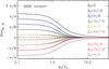 |
Fig. 6 Average bias on 106 MC noise simulations on |
3.4. Joint impact of the (Q,U) ellipticity and of the distribution of the true angles
In this section, we study the simultaneous impact of the shape of the noise covariance matrix and of the distribution of the true angles on the estimation of .
Montier et al. (2015a) showed that if the effective ellipticity between noise levels on Q and U differs from 1, then the bias on the polarization angle ψ oscillates depending on the true angle ψ0. The period of the oscillations is about π/ 2 (see their Fig. 14). Thus, if there is a true difference Δψ0,i = π/ 4 between angles ψ0(x) and ψ0(x + li), their respective biases can maximize the total difference Δψi for some pairs. Note if the noise components on Q and U are correlated (i.e., ρ ≠ 0),  will remain the value that yields the largest relative bias, while only the overall pattern would be shifted along ψ0.
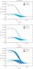 |
Fig. 7 Average bias on 106 MC realizations of the conventional estimator of the polarization angle dispersion function. Blue filled and red hashed areas delimit dispersion over 10 different sets of the true angles distributed randomly (blue) and uniformly (red) in three regimes of the shape of the noise covariance matrix, from top to bottom: canonical, low, extreme regimes. |
We run numerical simulations for the true value that would maximize the bias between pairs of angles in the case εeff ≠ 1. We also explore  for illustration purposes. We show in Fig. 7 the average bias for the uniform and random configuration of the true angles in the canonical, low and extreme regimes. For εeff ≠ 1 (i.e., in the low and extreme regimes), the dispersion in the bias appears for both configurations, which is represented by the vertical width of the curves in the middle and bottom panels in Fig. 7. In the low regime, the uniform configuration of the true angles gives a dispersion that is lower than the dispersion in the random configuration for . However, in the extreme regime the situation is the opposite. This can be due to the fact that in the uniform configuration, the imposed is valid for every pair of angles, thus giving
  , so that the relative bias between angles in a pair is maximized for some of the combinations. When angles are distributed randomly, is ensured for the ensemble, but not for each pair: the pairs of angles with little relative bias diminish the final result. For and for other
  (not shown here), the observed difference between the random and uniform cases in the three regimes of εeff is less prominent than for , but the overall behavior does not change.
The joint impact of the distribution of the true angles and the shape of the noise covariance matrix on the bias of is high at intermediate S/N. In the extreme regime and in the uniform configuration, the dispersion in the bias with respect to the canonical case reaches its maximum of 10.1° (≃π/ 18) at p0/σp = 2. This is not far from the value of the dispersion due to variations of the effective ellipticity only, given by the width of the grey area for in Fig. 3 (8.9°, ≃π/ 20). On the contrary, the dispersion in the bias in the random configuration gives only 6.4° (≃π/ 28) in the same S/N range. Thus, if the angles become random, it has little impact on the bias in the extreme regime. In the low regime and random configuration, the maximum dispersion in the bias is 4.2° (≃π/ 43) at p0/σp = 2, while it is equal to 1.5° (π/ 120) in the uniform configuration. Such a behavior of the bias can have a particularly strong impact on the estimation of . If one considers a polarization pattern where angles become decorrelated with the distance, so that close to the pixel of interest, angles are more or less similar and they become random with the distance. In that case, the angles close to the pixel for which the polarization angle dispersion function is calculated, will be affected more by the bias (positive or negative) due to the distribution of true angles than those which are farther. This would lead to a non-homogeneity in the estimation of the polarization angle dispersion function in both low and extreme regimes of the noise covariance matrix. Such an issue will not arise if one considers the polarization angle dispersion function calculated at a given lag,  , and if the width of the annulus is small compared to the typical scale for decorrelation of angles
3.5. Conventional uncertainties
As soon as the uncertainties of each of the angles ψ(x) and ψ(x+li) can be derived, one can obtain an estimate of the uncertainty on using the partial derivatives method. Such an estimator of the uncertainty will be called the “conventional” estimator hereafter. The conventional uncertainty of is given by (see Appendix A for derivation): ![Mathematical equation: \begin{eqnarray} \sigcl &= & \dfrac {1}{N \dpsi (\vec{x},l)} \left[\left(\sum_{i=1}^{N}[\psi (\vec{x}) - \psi (\vec{x} +\vec{l}_{i} )]\right)^{2} \sigma^{2}_{\psi(\vec{x})} \right.\\&&\left. + \sum_{i=1}^{N} [\psi (\vec{x}) - \psi (\vec{x} +\vec{l}_{i} )]^{2} \sigma^{2}_{\psi(\vec{x+l_{\it i}})} \right]^{1/2}. \label{eq:uncertainty} \end{eqnarray}](/articles/aa/full_html/2016/11/aa28809-16/aa28809-16-eq180.png) Although the conventional method is limited to relatively high S/Ns to ensure small deviations from the true value, it is the easiest method to derive an uncertainty on once the data and the associated noise information for each component are available. In order to quantify to which extent the conventional uncertainty can be reliable, we compare it to the uncertainty on given by the standard deviation of the distribution, denoted by
Although the conventional method is limited to relatively high S/Ns to ensure small deviations from the true value, it is the easiest method to derive an uncertainty on once the data and the associated noise information for each component are available. In order to quantify to which extent the conventional uncertainty can be reliable, we compare it to the uncertainty on given by the standard deviation of the distribution, denoted by  . The ratio of these uncertainties is shown in Fig. 8 in the canonical, low, and extreme regimes. Uncertainties on the angles,
  ,
,  , used in the determination of
  , are also calculated by the conventional method (Montier et al. 2015a) using Q and U and noise covariance matrices Σp,i of each pixel. Then, one should note that σψ(x) and σψ(x+li) are themselves subject to the limitation of the derivatives method.
At low S/N (p0/σp< 1), the estimate of the uncertainty using the conventional method is very inaccurate. In the canonical case of the noise covariance matrix, rapidly converges toward the true uncertainty and becomes compatible within 10% in the range p0/σp ∈ [1, 3]. Then it increases at higher S/N and overestimates the uncertainty on polarization angle dispersion function up to 38% at high (larger than 20) S/N of p. The ratio does not converge to 1 at high S/Ns. In the case of more complex shapes of the noise covariance matrix, can deviate from the true value by a factor of two at S/Ns ranging between 1 and 10. At S/N larger than 10, the ellipticity and correlation between Q and U do not affect the estimation of the uncertainty and becomes equal to that in the canonical regime.
The uncertainty on the polarization angle dispersion function determined by the conventional method can be used at S/N larger than one in the canonical case of the noise covariance matrix and gives a very conservative estimate of the true uncertainty.
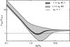 |
Fig. 8 Ratio between the conventional uncertainty and the true uncertainty of polarization angle dispersion function for different configurations of the noise covariance matrix. The dashed line represents the value of 1. |
4. Other estimators
4.1. Dichotomic estimator
The bias on the polarization angle dispersion function occurs because of the non-linearity in the Eq. (5) when deriving from the Stokes parameters. In order to overcome this issue, one can use the dichotomic estimator that consists of combining two independent measurements of the same quantity. The square of the dichotomic estimator of the polarization angle dispersion function has the following form: ![Mathematical equation: \begin{equation} \hat{\dpsi^{2}_{\rm D}} (\vec{x},l) = \frac{1}{N(l)} \sum_{i=1}^{N(l)} \left[\psi_{1}(\vec{x}) - \psi_{1} (\vec{x}+\vec{l}_i ) \right] \left[(\psi_{2}(\vec{x}) - \psi_{2} (\vec{x}+\vec{l}_i )) \right] , \end{equation}](/articles/aa/full_html/2016/11/aa28809-16/aa28809-16-eq193.png) (18)where subscripts 1 and 2 correspond respectively to each of the two data sets. We simulated the behavior of the dichotomic estimator of
(18)where subscripts 1 and 2 correspond respectively to each of the two data sets. We simulated the behavior of the dichotomic estimator of  by assuming the noise level of the two data sets to be
  times lower than the noise level considered for the conventional estimator . This allowed us to reproduce the situation where the original data had been divided in two subsets, so that σp becomes
  (as in the case of the Planck satellite data). The true angles were considered to be in the uniform configuration and the noise covariance matrix was in the canonical regime. Figure 9 shows the examples of the DFs of
  for
for  and
and  . At low S/Ns, the mean estimate of the DFs,
  tends to 0. The same trend is observed for any . The average bias for different values of is shown in Fig. 10. We conclude that the dichotomic estimator of the polarization angle dispersion function is always negatively biased.
The dichotomic estimator is not suitable for accurate estimate of the polarization angle dispersion function because it is a quadratic function that can take negative values. However, as its behavior is opposite to that of in the range ![Mathematical equation: \hbox{$\dpsiz \, \in \, [0, \randval]$}](/articles/aa/full_html/2016/11/aa28809-16/aa28809-16-eq203.png) , it can be used as a verification of the validity of :
, it can be used as a verification of the validity of :
-
if
 and
and  , then the noise level is low, is larger than , and gives a reliable estimate of ;
 -
if
and  , then the noise level is high and is probably larger than . In this case we suggest to estimate the upper limit of the bias as described in Sect. 4.4;
 -
if
 and , then is smaller than . We propose to use a polynomial combination of both
  and to better estimate (see Sect. 4.3) if two independent data sets are available, or to estimate the upper limit of the bias as described in Sect. 4.4.
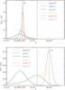 |
Fig. 9 Examples of the distribution function of the dichotomic estimator |
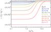 |
Fig. 10 Average bias on 106 MC realizations of the dichotomic estimator |
4.2. Bayesian DFs of
In an attempt to develop an accurate estimator of the polarization angle dispersion function, we use the difference between the behaviors of the conventional and dichotomic estimators in the range ![Mathematical equation: \hbox{$\dpsiz \in [0, \randval]$}](/articles/aa/full_html/2016/11/aa28809-16/aa28809-16-eq210.png) . In order to obtain knowing and from the data, we use the Bayes’ theorem. The posterior DF of can be given by
. In order to obtain knowing and from the data, we use the Bayes’ theorem. The posterior DF of can be given by 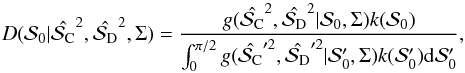 (19)where
  is a prior on , which we choose to be flat in the range [0,π/ 2]. Here,
  is the distribution function of the conventional and dichotomic estimators knowing the true polarization angle dispersion function and the noise covariance matrix.
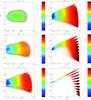 |
Fig. 11 Average of |
We numerically built the posterior DFs  for different values of and different S/N in the canonical regime. For this purpose, we first defined a two-dimensional grid G of the size Nc × Nd where Nc and Nd are the numbers of sampling of the squared conventional and dichotomic estimators in the ranges [0,(π/ 2)2] and [− (π/ 2)2,(π/ 2)2], respectively. Nc and Nd were chosen in a way to make sure that the meshes of the grid are squares with the size of 0.00826rad2 (Nc = 300, Nd = 600). Second, we run MC simulations for
 ![Mathematical equation: \hbox{$\dpsiz \, \in \, [0, \, \pi/2]$}](/articles/aa/full_html/2016/11/aa28809-16/aa28809-16-eq228.png) as previously. For each we performed NMC = 106 noise realizations in the canonical case of the noise covariance matrix, giving NMC pairs of
as previously. For each we performed NMC = 106 noise realizations in the canonical case of the noise covariance matrix, giving NMC pairs of  , where k ∈ [1,NMC]. After each run k, the corresponding was attributed to the mesh of the grid with coordinates . Finally, we averaged over in each mesh and obtain a grid of
  .
.
Examples of for different S/Ns in the canonical case of Σp are shown in Fig. 11. We note that, at very low S/N (top left panel) almost all combinations of the two estimators give distributed around π/ 4. Because of the noise, both estimators fail to correctly estimate and all possible give π/ 4 on average. But already at p0/σp = 1 (middle left panel), there is a correlation between and and small variations of with appear. At intermediate S/N (p0/σp = 2, 3, bottom left and top right panels respectively) the dependence of on is the most marked: is correlated with for any . In fact, as the posterior approach forces to be positive, and as is positive by definition, this explains that depends strongly on the conventional estimator. Also, high-value are difficult to obtain at low and intermediate S/N as it tends to 0 in presence of noise. On the contrary, the dependence of on the dichotomic estimator is stronger at low  and low (dark blue to light blue variations in panels corresponding to p0/σp = 1, 2, 3). At higher S/N (p0/σp> 5, center and bottom right panels), there is a strong correlation of with both and . At these S/N, takes positive values for moderate , but as soon as approaches π/ 2, is not efficient and we observe a feather-like pattern. We note that some values of and are never reached, or, in other words, there are values of and which do not give any . We would like to emphasize that the empirical Bayesian approach used here never gives 0 even at low (
 ) as this method averages over the values defined between 0 and π/ 2.
4.3. Polynomial estimator
In order to be able to directly use the conventional and dichotomic estimators of , without computing the Bayesian Posterior DFs, we search for a polynomial combination of and which would reflect the above simulations. To do so, we fitted the surface by a polynomial of the following form: 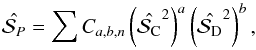 (20)where a ∈ [0,n], b ∈ [0,n] and n is the order of the polynomial. Thus, for each S/N and a given order, one would have the corresponding coefficients Ca,b,n. By applying these coefficients to any couple
  at a given S/N, one should be able to obtain the polynomial estimator
  .
.
Polynomial orders from 1 to 6 have been tested via comparison of the estimator to the result of the simulations . We focused on the case of the intermediate S/N (p0/σp = 2), as it corresponds to the regime where the bias on is the most affected by irregularities in the shape of Σp. The polynomial order 4 is the best compromise between the order of the polynomial degree and the goodness of the fit.
Once Ca,b,n are known, one can apply them to any couple of the measured estimators  in order to calculate the polynomial estimator. Nonetheless, one should be cautious about unrealistic values such as low and high , where no correct result can exist.
The average biases of the polynomial and conventional estimators in the canonical regime and uniform configuration of the true angles are compared in Fig. 12 for different S/Ns and . In the range ![Mathematical equation: \hbox{$\dpsiz \in [0, \pi/\!\!\sqrt{12}]$}](/articles/aa/full_html/2016/11/aa28809-16/aa28809-16-eq254.png) , the conventional estimator biases positively, while the dichotomic one negatively: their contributions are opposite, and gives more reliable results and performs better than at low and intermediate S/Ns. For example, at p0/σp = 2, the bias on is as high as 88% of the bias on at and it vanishes completely towards . Beyond the S/N of 4, the polynomial estimator is less accurate than the conventional one. For
, the conventional estimator biases positively, while the dichotomic one negatively: their contributions are opposite, and gives more reliable results and performs better than at low and intermediate S/Ns. For example, at p0/σp = 2, the bias on is as high as 88% of the bias on at and it vanishes completely towards . Beyond the S/N of 4, the polynomial estimator is less accurate than the conventional one. For ![Mathematical equation: \hbox{$\dpsiz \in [\pi/\!\!\sqrt{12}, \pi/2]$}](/articles/aa/full_html/2016/11/aa28809-16/aa28809-16-eq256.png) , the bias for both conventional and dichotomic estimators is negative and fails compared to the conventional estimator, as expected.
, the bias for both conventional and dichotomic estimators is negative and fails compared to the conventional estimator, as expected.
In this study, contributions of and  have been supposed to be equal, because is not known a priori. As a step forward, one can iterate on priors on and in order to improve the estimation of . When the first approximate result is obtained and the tendency with respect to high/low is recognized, one could attribute more or less weight to the estimator that is effective in that range of .
4.4. Estimation of the upper limit of the bias on 
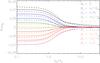 |
Fig. 12 Average bias on 106 MC realizations on conventional (dashed curves) and polynomial (plain curves) estimators in the canonical case of covariance matrix (εeff = 1) for various |
When the dichotomic estimator cannot be calculated, that is, there is only one measurement per spatial position, it is helpful to evaluate to which extent one can trust the conventional estimator, given by Eq. (5). We propose a simple test that consists of calculating the maximum bias due to the noise of the data.
As seen in Sect. 3, the largest bias occurs for . A MC noise simulation consistent with the noise covariance matrices of the data at would give the value of the maximum possible bias. For that purpose we need to change I, Q and U in such a manner as to have , and we keep the S/N of p unchanged. The only way to have is to attribute the same true polarization angle for all the pixels inside the considered area. Such a configuration is given by  (21)where r is a real constant,
  and
and  are the Stokes parameters which will be used in the calculation of the upper limit on the bias on the polarization angle dispersion function. The total intensity should also be modified in order to preserve p. It is given by
 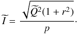 (22)The system for (
 ) can be closed if we adopt an expression for σp. We consider σp as given by the conventional uncertainty estimator with no cross-correlation terms:
 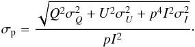 (23)Then, the new Stokes Q parameter is given by
 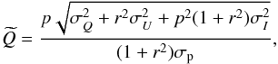 (24)and the expression of the new Stokes U parameter is the following:
  (25)For example, we took the true value
  in the uniform configuration of the true angles and the effective ellipticity εeff = 1.1 (low regime) with ε = 1.1 and ρ = 0. We assumed the total intensity I0 to be equal to 1 and perfectly known as in the above simulations, so that we dealt with the reduced noise covariance matrix (see Eq. (11). We also assumed the uncertainty σU = U0, then σQ = εσU = 1.1σU from Eq. (10). This allowed us to build the simulated noise covariance matrix Σp. We simulated a measurement by running one noise realization consistent with Σp and obtained
  . We followed the above-described procedure and, averaging over 106 noise realizations we obtained the mean value of the maximum bias ⟨ Biasmax ⟩ = 21.5° with the standard deviation σ(Biasmax) = 7.5°. Thus, in this case, the estimation of can be affected by bias almost by the same order of magnitude as the true value. This method can not be directly used to “de-bias” the conventional estimator but can be used to estimate, on average, at which level the estimation of the polarization angle dispersion function is affected by the noise level and the shape of the noise covariance matrix.
5. Discussion and conclusion
In this paper, we studied the bias on the polarization angle dispersion function and we have demonstrated its complex behavior for the first time. We showed that it strongly depends on the true value which is not known a priori: the bias on the conventional estimator is negative for  (≃52°), which is the value corresponding to the result if all the angles considered in the calculation are random, positive for
  , and it can reach up to at low S/Ns (Sect. 3.1). The bias on the polarization angle dispersion function also depends on the shape of the noise covariance matrix and the distribution of the true angles in the intermediate range of S/N, between 1 and 4 as seen in Sects. 3.2, 3.3. However, if there is less than 10% effective ellipticity between noise levels on Stokes parameters Q and U, the impact of the shape of the noise covariance matrix and of the distribution of the true angles can be neglected. Otherwise, these factors can significantly affect the estimation of the polarization angle dispersion function when using the conventional estimator.
We have introduced the dichotomic estimator of and studied its behavior. We showed that the bias on is always negative. In addition, such an estimator has the disadvantage of being a quadratic function that can take negative values. However, using both conventional and dichotomic estimators appears to be the first step in assessing the true value of the polarization angle dispersion function. We have introduced a new polynomial estimator that allows us to use the low S/N data (less than 4). This broadens the application of the polarization angle dispersion function in different polarimetric studies. Yet deriving the polynomial estimator requires the existence of at least two independent measurements as well as an additional computational time to run simulations.
We propose a method to evaluate the maximum possible bias of the polarization angle dispersion function knowing the noise covariance matrix of the data. It can be used as an estimator of the upper limit to the bias on with any polarimetric data with the available noise covariance matrices in (Q,U).
The methods developed in this work (maximum bias estimation and dichotomic estimator) have been applied to the Planck data in order to analyze the observed dust polarization with respect to the magnetic field structure. Planck Collaboration Int. XIX (2015) calculates the polarization angle dispersion function in an annulus of a 30′ lag and 30′ width all over the sky at 1° resolution, revealing filamentary features. Using the dichotomic estimator and the test of the maximum bias on , Planck Collaboration Int. XIX (2015) demonstrates that these filamentary features are not artifacts of noise. Moreover, a clear anti-correlation between the polarization fraction and the polarization angle dispersion function has been shown.
Planck Collaboration Int. XIX (2015) uses the data smoothed to 1° resolution, which diminishes the noise level. Also, as the effective ellipticity of the Planck data deviates at most by 12% from the canonical case (Planck Collaboration Int. XIX 2015), the shape of the noise covariance matrix has been taken into account in the estimation of . The results of this work can also be particularly well suited in the analysis of the data from the new experiments that are designed for polarized emission studies, such as the balloon-borne experiments BLAST-Pol (Fissel et al. 2010), PILOT (Bernard et al. 2007) and the ground-based telescopes with new polarization capabilities: ALMA (Pérez-Sánchez & Vlemmings 2013), SMA, NIKA2 (Catalano et al. 2016). We suggest to calculate both the conventional and dichotomic estimators in order to compare both, in the case where two independent data-sets are available, as well as to estimate the upper limit of the bias on using the method proposed in this work for any polarimetric data with the noise covariance matrix provided. A joint IDL/Python library which includes the methods from the work on bias analysis and estimators of polarization parameters is currently under development.
References
- Andersson, B.-G., Lazarian, A., & Vaillancourt, J. 2015, ARA&A, 53, 501 [NASA ADS] [CrossRef] [Google Scholar]
- Beck, R., & Gaensler, B. 2004, New Astron. Rev., 48, 1289 [Google Scholar]
- Benoît, A., Ade, P., Amblard, A., et al. 2004, A&A, 424, 571 [NASA ADS] [CrossRef] [EDP Sciences] [Google Scholar]
- Bernard, J.-P., Ade, P., De Bernardis, P., et al. 2007, EAS Pub. Ser., 23, 189 [CrossRef] [EDP Sciences] [Google Scholar]
- Catalano, A., Adam, R., Ade, P., et al. 2016, ApJ, submitted [arXiv:1605.08628] [Google Scholar]
- Chandrasekhar, S., & Fermi, E. 1953, ApJ, 118, 113 [NASA ADS] [CrossRef] [Google Scholar]
- Cortes, P., Girart, J., Hull, C., et al. 2016, ApJ, 825, 15 [Google Scholar]
- Crutcher, R., Nutter, D., Ward-Thompson, D., & Kirk, J. 2004, ApJ, 600 [Google Scholar]
- Davis, L., & Greenstein, J. 1951, ApJ, 114, 206 [Google Scholar]
- Dotson, J., Vaillancourt, J., Kirby, L., Dowell, C., & Hildebrand, R. 2010, ApJ, 186, 406 [NASA ADS] [Google Scholar]
- Falceta-Gonçalves, D., Lazarian, A., & Kowal, G. 2008, ApJ, 679, 537 [NASA ADS] [CrossRef] [Google Scholar]
- Fissel, L. M., Ade, P. A. R., Angilé, F. E., et al. 2010, in Proc. SPIE, 7741 [Google Scholar]
- Fletcher, A. 2010, in ASP Conf. Ser. 438, eds. R. Kothes, T. Landecker, & A. Willis, 197 [Google Scholar]
- Girart, J. M., Rao, R., & Marrone, D. P. 2006, Science, 313, 812 [NASA ADS] [CrossRef] [PubMed] [Google Scholar]
- Hall, J., & Mikesell, A. 1949, AJ, 54, 187 [NASA ADS] [CrossRef] [Google Scholar]
- Han, J. 2002, Chin. J. Astron. Astrophys., 2, 293 [Google Scholar]
- Heiles, C. 1996, ApJ, 462, 316 [NASA ADS] [CrossRef] [Google Scholar]
- Heiles, C., & Troland, T. 2005, ApJ, 624, 773 [NASA ADS] [CrossRef] [Google Scholar]
- Hildebrand, R., Kirby, L., Dotson, J., Houde, M., & Vaillancourt, J. 2009, ApJ, 696, 567 [NASA ADS] [CrossRef] [Google Scholar]
- Hiltner, W. 1949, ApJ, 109, 471 [NASA ADS] [CrossRef] [Google Scholar]
- Hiltner, W. 1951, ApJ, 114, 241 [NASA ADS] [CrossRef] [Google Scholar]
- Houde, M., Rao, R., Vaillancourt, J., & Hildebrand, R. 2011a, ApJ, 733, 109 [NASA ADS] [CrossRef] [Google Scholar]
- Houde, M., Vaillancourt, J., Hildebrand, R., Chitsazzadech, S., & Kirby, L. 2011b, ApJ, 706, 1504 [Google Scholar]
- Houde, M., Hull, C., Plambeck, R., Vaillancourt, J., & Hildebrand, R. 2016, ApJ, 820, 38 [NASA ADS] [CrossRef] [Google Scholar]
- Lai, S.-P., Crutcher, R. M., & Girart, J. M. 2001, BAAS, 33, 1360 [NASA ADS] [CrossRef] [Google Scholar]
- Lazarian, A., & Hoang, T. 2008, ApJ, 676, L25 [NASA ADS] [CrossRef] [Google Scholar]
- Mao, S., Gaensler, B., Haverkorn, M., et al. 2010, ApJ, 714, 1170 [NASA ADS] [CrossRef] [Google Scholar]
- Mathewson, D., & Ford, V. 1970, MmRAS, 74, 139 [Google Scholar]
- Matthews, B., McPhee, C., Fisse, L., & Curran, R. 2009, ApJ, 182, 143 [Google Scholar]
- Montier, L., Plaszczynski, S., Levrier, F., et al. 2015a, A&A, 574, A135 [NASA ADS] [CrossRef] [EDP Sciences] [Google Scholar]
- Montier, L., Plaszczynski, S., Levrier, F., et al. 2015b, A&A, 574, A136 [NASA ADS] [CrossRef] [EDP Sciences] [Google Scholar]
- Pérez-Sánchez, A., & Vlemmings, W. 2013, A&A, 551, A15 [NASA ADS] [CrossRef] [EDP Sciences] [Google Scholar]
- Planck Collaboration Int. XIX. 2015, A&A, 576, A104 [NASA ADS] [CrossRef] [EDP Sciences] [Google Scholar]
- Poidevin, F., Bastien, P., & Matthews, B. 2010, ApJ, 716, 893 [NASA ADS] [CrossRef] [Google Scholar]
- Quinn, J. 2012, A&A, 538, A65 [NASA ADS] [CrossRef] [EDP Sciences] [Google Scholar]
- Sandstrom, K. M., Latham, D. W., Torres, G., Landsman, W. B., & Stefanik, R. P. 2002, BAAS, 34, 1300 [NASA ADS] [Google Scholar]
- Serkowski, K. 1958, Acta Astron., 8, 135 [NASA ADS] [Google Scholar]
- Simmons, J., & Stewart, B. 1985, A&A, 142, 100 [NASA ADS] [Google Scholar]
- Tang, Y.-W., Ho, P., Koch, P., Guilloteau, S., & Dutrey, A. 2012, Proc. Magnetic Fields in the Universe [Google Scholar]
- Vaillancourt, J. 2007, EAS Pub. Ser., 23, 147 [CrossRef] [EDP Sciences] [Google Scholar]
- Vaillancourt, J. E. 2006, PASP, 118, 1340 [Google Scholar]
- Wardle, J., & Kronberg, P. 1974, ApJ, 194, 249 [NASA ADS] [CrossRef] [Google Scholar]
- Zhang, Q., Qiu, K., Girart, J., et al. 2010, PASP, 792, 116 [Google Scholar]
Appendix A: Derivation of the conventional uncertainty
We assume the uncertainties on angles to be known. Let start by the definition of variance applied to and consider small displacement of : ![Mathematical equation: \appendix \setcounter{section}{1} \begin{equation} \sigma^{2}_{\dpsi (\vec{x},l) } = E \left[(\dpsi (\vec{x},l) - E \left[\dpsi \left(\vec{x},l\right)\right] )^{2}\right] = E \left[({\rm d} \dpsi (\vec{x},l))^{2} \right]. \end{equation}](/articles/aa/full_html/2016/11/aa28809-16/aa28809-16-eq284.png) (A.1)The differential of includes partial derivatives with respect to the angle at position x and each angle at positions x + li, with i ∈ [1,N]:
(A.1)The differential of includes partial derivatives with respect to the angle at position x and each angle at positions x + li, with i ∈ [1,N]: ![Mathematical equation: \appendix \setcounter{section}{1} \begin{equation} {\rm d}\dpsi (\vec{x},l ) =\dfrac {\partial \dpsi (\vec{x},\vec{l}) } {\partial \psi (\vec{x}) } {\rm d} \psi (\vec{x}) + \sum_{i=1}^{N} \left[\dfrac { \partial \dpsi }{\partial \psi (\vec{x}+\vec{l_{\it i}} ) } {\rm d} \psi (\vec{x}+\vec{l_{\it i}} )\right]. \end{equation}](/articles/aa/full_html/2016/11/aa28809-16/aa28809-16-eq287.png) (A.2)When developing the square, one has:
(A.2)When developing the square, one has:  (A.3)If one takes the expectation of
  , then
 ![Mathematical equation: \appendix \setcounter{section}{1} \begin{eqnarray} E [{\rm d}\dpsi (\vec{x},l ) ^ {2}]& \ = \ & \left( \dfrac {\partial \dpsi (\vec{x},l) } {\partial \psi (\vec{x}) } \right) ^{2} \, \sigma^{2}_{ \psi (\vec{x})} + \sum_{i=1}^{N} \, \left( \dfrac { \partial \dpsi (\vec{x}, l )}{\partial \psi (\vec{x}+\vec{l_{\it i}} ) } \right) ^ {2} \,\sigma^{2}_{\psi (\vec{x+l_{\it i}})} \nonumber \\ &&\,+ 2 \, \sum_{i=1}^{N} \, \dfrac {\partial \dpsi (\vec{x},l) } {\partial \psi (\vec{x}) } \dfrac { \partial \dpsi (\vec{x}, l )}{\partial \psi (\vec{x}+\vec{l_{\it i}} ) } \, \sigma_{\psi (\vec{x}) \psi (\vec{x+l_{\it i}}) }. \label{eq:dpsi_sig_full2} \end{eqnarray}](/articles/aa/full_html/2016/11/aa28809-16/aa28809-16-eq290.png) (A.4)The partial derivatives are:
(A.4)The partial derivatives are: ![Mathematical equation: \appendix \setcounter{section}{1} \begin{eqnarray*} \dfrac{\partial \dpsi (\vec{x},l ) } {\partial \psi (\vec{x}) } \!= \!\dfrac{1}{2} \, \left( \dfrac{1}{N} \sum_{i=1}^{N} \,[\psi (\vec{x}) -\psi (\vec{x+l_{\it i}})]^{2} \right)^{-1/2 } \left( \dfrac{2}{N}\, \sum_{i=1}^{N} \, [\psi (\vec{x}) \!-\! \psi (\vec{ x+l_{i} }] \right), \end{eqnarray*}](/articles/aa/full_html/2016/11/aa28809-16/aa28809-16-eq291.png)
![Mathematical equation: \appendix \setcounter{section}{1} \begin{eqnarray*} \dfrac {\partial \dpsi (\vec{x},l ) } {\partial \psi (\vec{x+l_{\it i}}) } = - \dfrac{1}{2} \, \left( \dfrac{1}{N} \sum_{i=1}^{N} \, [\psi (\vec{x}) - \psi (\vec{x} +\vec{l}_{i} )]^{2} \right)^{-1/2 } \dfrac{2}{N} \left(\psi (\vec{x}, \vec{l} )\! - \!\psi (\vec{x} \!+ \!\vec{l}_{i} )\right); \end{eqnarray*}](/articles/aa/full_html/2016/11/aa28809-16/aa28809-16-eq292.png)
![Mathematical equation: \appendix \setcounter{section}{1} \begin{eqnarray} \left(\dfrac{\partial \dpsi (\vec{x},l ) } {\partial \psi (\vec{x}) } \right) ^{2} & = & \dfrac{1}{N^{2}} \left( \dfrac{1}{N} \sum_{i=1}^{N} [\psi (\vec{x} ) - \psi (\vec{x} +\vec{l}_{i} )]^{2} \right)^{-1 } \nonumber \\ && \quad \times \, \left(\sum_{i=1}^{N}[\psi (\vec{x}) - \psi (\vec{x} +\vec{l}_{i} )]\right)^{2} \nonumber \\ & =& \dfrac { \left(\sum_{i=1}^{N}[\psi (\vec{x}) - \psi (\vec{x} +\vec{l}_{i} )] \right)^{2} } { N^{2} [\dpsi (\vec{x},l)]^{2}} \\ \left(\dfrac {\partial \dpsi (\vec{x},l ) } {\partial \psi (\vec{x+l_{\it i}}) } \right) ^ {2} & =& \dfrac{ [\psi (\vec{x} ) - \psi (\vec{x} +\vec{l}_{i} )]^{2} }{N^{2}[\dpsi (\vec{x},l)]^{2}}\cdot \end{eqnarray}](/articles/aa/full_html/2016/11/aa28809-16/aa28809-16-eq293.png) As the noise levels on two measurements of polarization angle at different positions are uncorrelated, one has:
As the noise levels on two measurements of polarization angle at different positions are uncorrelated, one has:  Since
Since ![Mathematical equation: \hbox{$E [{\rm d}\dpsi (\vec{x},l ) ) ^ {2}] = \sigma^{2}_{\dpsi (\vec{x},l)}$}](/articles/aa/full_html/2016/11/aa28809-16/aa28809-16-eq295.png) , Eq. (A.3) becomes
, Eq. (A.3) becomes ![Mathematical equation: \appendix \setcounter{section}{1} \begin{eqnarray} \sigma^{2}_{\dpsi (\vec{x},l)}& = & \,\dfrac{1}{[N\dpsi (\vec{x},l)]^{2}} \left[\left(\sum_{i=1}^{N}\left[\psi (\vec{x}) - \psi (\vec{x} +\vec{l}_{i} ) \right] \right)^{2} \sigma^{2}_{\psi(x)} \right. \nonumber \\ & &\left. + \sum_{i=1}^{N} (\psi (\vec{x}) - \psi (\vec{x} +\vec{l}_{i} ) )^{2} \sigma^{2}_{\psi(\vec{x+l_{\it i}})} \right]. \end{eqnarray}](/articles/aa/full_html/2016/11/aa28809-16/aa28809-16-eq296.png) (A.7)Taking the square root of this expression, one gets the conventional uncertainty on polarization angle dispersion function:
(A.7)Taking the square root of this expression, one gets the conventional uncertainty on polarization angle dispersion function: ![Mathematical equation: \appendix \setcounter{section}{1} \begin{eqnarray} \sigcl& = & \,\dfrac {1}{N \dpsi (\vec{x},l)} \left [\left(\sum_{i=1}^{N}\left[\psi (\vec{x}) - \psi (\vec{x} +\vec{l}_{i} ) \right]\right)^{2} \sigma^{2}_{\psi(\vec{x})} \right.\nonumber \\ && \left.+ \sum_{i=1}^{N} \left[\psi (\vec{x}) - \psi (\vec{x} +\vec{l}_{i} ) \right]^{2} \sigma^{2}_{\psi(\vec{x+l_{\it i}})}\right]^{1/2}. \label{eq:uncertainty2} \end{eqnarray}](/articles/aa/full_html/2016/11/aa28809-16/aa28809-16-eq297.png) (A.8)
(A.8)
All Figures
|
Fig. 1 Schematic view of the simulated configuration of polarization orientations. The polarization angle dispersion function is calculated at the position of the red line segment within the red-dotted circle of radius l. Left: uniform configuration. Right: random configuration. Both cases give |
| In the text | |
|
Fig. 2 Examples of the simulated distribution functions of the conventional estimator of the dispersion function |
| In the text | |
|
Fig. 3 Average bias on 106 MC noise realizations for the conventional estimator |
| In the text | |
|
Fig. 4 Maximum absolute deviation of the bias induced by variations of the effective ellipticity between noise in (Q, U) and the true value |
| In the text | |
|
Fig. 5 Standard deviation of the difference between the true angle ψ0,0 and the true angles ψ0,i,i ∈ [1,9] as a function of the true polarization angle dispersion function |
| In the text | |
|
Fig. 6 Average bias on 106 MC noise simulations on |
| In the text | |
|
Fig. 7 Average bias on 106 MC realizations of the conventional estimator of the polarization angle dispersion function. Blue filled and red hashed areas delimit dispersion over 10 different sets of the true angles distributed randomly (blue) and uniformly (red) in three regimes of the shape of the noise covariance matrix, from top to bottom: canonical, low, extreme regimes. |
| In the text | |
|
Fig. 8 Ratio between the conventional uncertainty and the true uncertainty of polarization angle dispersion function for different configurations of the noise covariance matrix. The dashed line represents the value of 1. |
| In the text | |
|
Fig. 9 Examples of the distribution function of the dichotomic estimator |
| In the text | |
|
Fig. 10 Average bias on 106 MC realizations of the dichotomic estimator |
| In the text | |
|
Fig. 11 Average of |
| In the text | |
|
Fig. 12 Average bias on 106 MC realizations on conventional (dashed curves) and polynomial (plain curves) estimators in the canonical case of covariance matrix (εeff = 1) for various |
| In the text | |
Current usage metrics show cumulative count of Article Views (full-text article views including HTML views, PDF and ePub downloads, according to the available data) and Abstracts Views on Vision4Press platform.
Data correspond to usage on the plateform after 2015. The current usage metrics is available 48-96 hours after online publication and is updated daily on week days.
Initial download of the metrics may take a while.