| Issue |
A&A
Volume 573, January 2015
|
|
|---|---|---|
| Article Number | A110 | |
| Number of page(s) | 8 | |
| Section | Extragalactic astronomy | |
| DOI | https://doi.org/10.1051/0004-6361/201424235 | |
| Published online | 07 January 2015 | |
Lower mass normalization of the stellar initial mass function for dense massive early-type galaxies at z ~ 1.4
1 INAF – Osservatorio Astronomico di Brera, via Brera 28, 20121 Milan, Italy
e-mail: This email address is being protected from spambots. You need JavaScript enabled to view it.
2 Dipartimento di Scienza e Alta Tecnologia, Università degli Studi dell’Insubria, via Valleggio 11, 22100 Como, Italy
Received: 19 May 2014
Accepted: 16 October 2014
Abstract
Aims. This paper aims at understanding whether the normalization of the stellar initial mass function (IMF) of massive galaxies varies with cosmic time and/or with mean stellar mass density Σ = M⋆/(2πRe2).
Methods. We have tackled this question by taking advantage of a spectroscopic sample of 18 dense (Σ > 2500 M⊙ pc-2) massive early-type galaxies (ETGs) that we collected at 1.2 ≲ z ≲ 1.6. Each galaxy in the sample was selected in order to have available: i) a high-resolution deep HST-F160W image to visually classify it as an ETG; ii) an accurate velocity dispersion estimate; iii) stellar mass derived through the fit of multiband photometry; and iv) structural parameters (i.e. effective radius Re and Sersic index n) derived in the F160W-band. We have constrained the mass-normalization of the IMF of dense high-z ETGs by comparing the true stellar masses of the ETGs in the sample (Mtrue) derived through virial theorem, hence IMF independent, with those inferred through the fit of the photometry which assume a reference IMF (Mref). Adopting the virial estimator as proxy of the true stellar mass, we have implicitly assumed that these systems have zero dark matter. However, recent dynamical analysis of massive local ETGs have shown that the dark matter fraction within Re in dense ETGs is negligible (<5−10%) and simulations of dissipationless mergers of spheroidal galaxies have shown that this fraction decreases going back with time. Accurate dynamical models of local ETGs performed by the ATLAS3D team have shown that the virial estimator is prone to underestimating or overestimating the total masses. We have considered this, and based on the results of ATLAS3D we have shown that for dense ETGs the mean value of total masses derived through the virial estimator with a non-homologous virial coefficient and Sersic-Re are perfectly in agreement with the mean value of those derived through more sophisticated dynamical models, although, of course, the estimates show higher uncertainties.
Results. Tracing the variation of the parameter Γ = Mtrue/Mref with velocity dispersion σe, we have found that, on average, dense ETGs at ⟨ z ⟩ = 1.4 follow the same IMF-σe trend of typical local ETGs, but with a lower mass-normalization. The observed lower normalization could be evidence of i) an evolution of the IMF with time or ii) a correlation with Σ. To discriminate between the two possibilities, we have compared the IMF-σe trend that we have found for high-z dense ETGs with that of local ETGs with similar mean stellar mass density and velocity dispersion and we have found that the IMF of massive dense ETGs does not depend on redshift. The similarity between the IMF-σe trends observed both in dense high-z and low-z ETGs over 9 Gyr of evolution and their lower mass-normalization with respect to the mean value of local ETGs suggests that, independently of formation redshift, the physical conditions which characterized the formation of a dense spheroid on average lead to a mass spectrum of newly formed stars with a higher ratio of high- to low-mass stars with respect to the IMF of normal local ETGs. In the direction of our findings, recent hydrodynamical simulations show that the higher star-formation rate that should have characterized the early stage of star formation of dense ETGs is expected to inhibit the formation of low-mass stars. Hence, compact ETGs should have higher ratio of high- to low-mass stars than normal spheroids, as we observe.
Key words: galaxies: elliptical and lenticular, cD / galaxies: evolution / galaxies: formation / galaxies: high-redshift / galaxies: stellar content
© ESO, 2015
1. Introduction
The stellar initial mass function (IMF) is the mass distribution of a stellar generation at birth; fixing the relative number of low- and high-mass stars formed in a burst of star formation, it determines the properties of the whole stellar system, i.e. its spectral energy distribution (SED), stellar mass, stellar mass-to-light ratio (M/L), chemical enrichment, and how these properties change with time. In fact, the most widely adopted approaches to constrain the assembly history of galaxies pass through the analysis of their stellar populations properties (e.g. stellar mass, age, star-formation histories) over the cosmic time. The properties of these stellar populations are derived, at different redshifts, by comparing observations with stellar population synthesis (SPS) models which strictly depend on the IMF. Consequently, the knowledge of the IMF is a key ingredient for our understanding of the stellar mass accretion over the cosmic time. Nowadays, the local direct star counts have shown that the IMF is approximately constant throughout the disk of the Milky Way (MW) and can be described by two declining power laws dN/dm∝m−s, one with slope s ≃ 2.35 for stars with mass m ≳ 1 M⊙, as originally suggested by Salpeter (1955), and the other, flatter, for lower masses (e.g. Kroupa 2001; Chabrier 2003). This form, measured in the MW disk, is then assumed to be universal, i.e. invariant both throughout the wide population of galaxies, and across the cosmic time. Nonetheless, theoretical arguments cast strong doubts on IMF universality (see Bastian et al. 2010; Kroupa et al. 2013, for complete reviews).
The Jeans mass MJ is dependent on the temperature T and the density ρ of the gas (MJ ∝ T3/2ρ− 1/2) (e.g. Larson 1998, 2005; Bonnell et al. 2006). The temperature of a gas is related to its metallicity Z: at fixed heating rate, the gas cooling efficiency is reduced in absence of metals, and consequently the gravitational collapse of low-mass stars is inhibited in metal poor gas (e.g. Larson 2005; Bate & Bonnell 2005; Bate 2005; Bonnell et al. 2006). In addition to this, there is evidence that the turbulence level of the interstellar medium plays a major role in shaping the IMF (e.g. Padoan & Nordlund 2002; Hennebelle & Chabrier 2008; Hopkins 2013). These theoretical considerations show that the mass spectrum of the stars formed in a burst of star formation is deeply connected with the physical properties of the gas cloud, and hence raise doubts about the validity of the current IMF universality assumption.
From an observational point of view, the IMF universality has recently been contrasted by indirect emerging evidence in external galaxies. The study of spectral features known to be sensitive to the presence of low-mass stars (e.g. the Na I doublet, the Ca II triplet) in massive local early-type galaxies (ETGs) have shown that the strength of these gravity-sensitive features varies with ETG velocity dispersion (σ) and the Mg/Fe ratio in the direction of progressively bottom-heavy IMF, i.e. IMF with a lower ratio of high- to low-mass stars than the MW IMF, with the increase of the two parameters (e.g. Conroy & van Dokkum 2012; Spiniello et al. 2012; Ferreras et al. 2013; La Barbera et al. 2013).
A similar IMF-σ trend has been found through a different (dynamical) approach based on the direct comparison of the true stellar mass-to-light ratio (M/L⋆,true) with that inferred through, e.g. the fit of the spectral energy distribution adopting SPS models which assume a fixed IMF as reference (M/L⋆,ref). The M/L⋆,true has been derived by different authors through, e.g. detailed 2D axisymmetric dynamical models (Cappellari et al. 2012), simpler spherical dynamical models (Tortora et al. 2013), or through a joint lensing and dynamical analysis of gravitational lenses (Treu et al. 2010). The two independent approaches have been shown to achieve a similar trend with velocity dispersion (Tortora et al. 2013; Conroy et al. 2013). This consolidates the robustness of the IMF-σ trend in local massive ETGs, although caveats and limits of both methods need to be fully understood yet (Smith 2014).
Nonetheless, the most relevant aspect for galaxy evolution, i.e. the assumption of a universality across the cosmic time, is still largely observationally unexplored. Theoretically, the higher temperature of intergalactic medium, which is known to increase with redshift as ∝2.73(1 + z)[K], should contrast the formation of low-mass stars at high redshift and hence point toward a top-heavier IMF in early epoch with respect to that of the local Universe (e.g. Larson 1998, 2005). Similarly, the formation of low-mass stars should be inhibited by the absence of metals in the primordial gas (e.g. Larson 2005), as well as by the higher star-formation rate per unit volume observed in the early universe (e.g. Larson 2005; Dabringhausen et al. 2010; Papadopoulos 2010; Papadopoulos et al. 2011; Narayanan & Davé 2012).
Actually, in a recent analysis, Shetty & Cappellari (2014) have provided the first attempt to constrain the IMF in massive (M⋆> 1011M⊙) ETGs at z ~ 0.8 using axisymmetric dynamical models. They find that, on average, the IMF of z ~ 0.8 ETGs is similar to those of local ones with similar stellar mass. This result is consistent with the evidences that, on average, the stellar content of ETGs passively evolves from z ~ 0.8 − 1 down to zero (e.g. di Serego Alighieri et al. 2005; van der Wel et al. 2005; Jørgensen & Chiboucas 2013; Choi et al. 2014). In fact, if a variation of IMF in massive ETGs occurs with time, it will be mostly detectable through the analysis of the stellar content of ETGs at z> 1. Actually, the number density of spheroidal massive galaxies increases by a factor ~10 in the range 1 <z< 2 and is almost flat at lower redshift (Ilbert et al. 2013). This, coupled with the many evidences of passive evolution of the stellar content of massive ETGs in the last 7−8 Gyr, implies that, on average, the mean properties of the stellar content of massive ETGs observed at z< 1 are not dissimilar to those observed in local ETGs. In contrast, the population of ETGs z ~ 1.5 provides us with information only on those spheroidal galaxies that assembled their stellar content in the first 3−4 Gyr of the age of the Universe. Consequently, they retain information on the mass spectrum of stars in the early Universe.
A piece of evidence concerning the stellar content of spheroidal galaxies up to z ~ 1.5, is that at fixed stellar mass M⋆, ETGs show a remarkable spread in mean stellar mass density (Σ = M⋆/2π ). Although conclusive results have not been achieved yet, a few recent works (e.g. Läsker et al. 2013; Smith & Lucey 2013) and theoretical expectations have suggested that the hotter dynamical status of a system could have a fundamental role in shaping the IMF (e.g. Dabringhausen et al. 2008, 2010; Papadopoulos 2010; Dabringhausen et al. 2012; Marks et al. 2012).
Total sample of ⟨ z ⟩ = 1.4 galaxies.
In this paper, taking advantage of a sample of ~18 dense (Σ > 2500 M⊙ pc-2) ETGs we have collected at 1.26 <z< 1.6 (see Sect. 2 for more details), we address the following questions: i) Does dense high-z ETGs follow the same IMF-σ trend observed for local ETGs? ii) Does the IMF of ETGs depend on mean stellar mass density and/or on redshift? In Sect. 3 we derive the upper limit of the IMF-σ trend of dense ETGs at ⟨ z ⟩ = 1.4. We infer the trend in dynamical masses derived via the virial estimator. Although this procedure is less accurate than the more sophisticated 2D axisymmetric model, in Sect. 3 we discuss in detail how the source of uncertainties could affect our conclusions. In Sect. 4 we present our discussion, and we summarize our results in Sect. 5.
Throughout the paper we adopt standard cosmology with H0 = 70 km s-1 Mpc-1, Ωm = 0.3 and Ωλ = 0.7.
2. The sample of dense ETGs at ⟨ z ⟩ = 1.4
The dataset we have adopted in this paper is a collection from the literature of all the 18 galaxies morphologically confirmed as ETGs at 1.26 <z< 1.6, having stellar mass density Σ > 2500 M⊙ pc-2, and both kinematic (i.e. velocity dispersion σe) and structural (i.e. effective radius Re and stellar mass M⋆) properties available. For all the galaxies in the sample, the morphological classification was performed on the basis of a visual inspection of the galaxies carried out on the HST-NIC2 and WFC3 images in the F160W filter. We classified as ETGs those galaxies having a regular shape with no sign of disk and no irregular or structured residuals resulting from the profile fitting. We selected only those ETGs with structural parameters derived by fitting the HST images with a point spread function-convolved 2D Sersic profile and with stellar masses derived with the Chabrier IMF and Bruzual & Charlot (2003) models. We consider that stellar masses have a typical error of ~20%, which take into account the uncertainties related to models and photometry, but not on IMF, that for the purpose of our study we consider fixed. In Table 1 we list all the properties of the 18 galaxies relevant for this analysis, i.e. the effective radii, the filter in which they were derived, the stellar masses, as well as their velocity dispersions within the effective radius. We rescaled the measured velocity dispersions to Re aperture following Cappellari et al. (2006). For 14 ETGs in the sample the values of both structural and kinematical parameters have already been published and we refer the reader to original papers for all the details (see references in Table 1), while for the remaining four (S2F1-511, S2F1-633, S2F1-527, S2F1-389) the estimates of velocity dispersions and the updated values of structural parameters will be presented in a forthcoming paper (Gargiulo et al. 2014). In the following paragraph we briefly describe the method used to derive the physical parameters of these four galaxies (hereafter our high-z sample galaxies).
2.1. Our high-z sample galaxies
We derived the velocity dispersions of the four galaxies at z ~ 1.3 from spectra obtained with the ESO VLT-FORS2 spectrograph. The OG590 filter and the GRIS-600z grism we chose for the observations, allowed us to cover the wavelength range 0.7 <λ< 1.0μm with a sampling of 1.6 Å per pixel. We fixed the width of the slit to 1”, which provides a resolution R ≃ 1400, corresponding to a FWHM ≃ 6.5 Å at 9000 Å. The total effective integration time per galaxy is ~8.5 h which results in a signal-to-noise per pixel ~[8−10]. After standard reduction and calibration, we derived the velocity dispersions best-fitting the observed spectra with a set of template stars from Munari et al. (2005) using the software pPXF (Cappellari & Emsellem 2004). With an extensive set of simulations we tested the reliability of our estimates, given the wavelength region covered and the signal-to-noise of the spectra and found that fitting the observed spectra with a Gauss+Hermite polynomial over the whole range of λ, with a penalty BIAS ≃ 0.1 provides reliable estimates of σ. The effective radii were derived by Longhetti et al. (2007) fitting the HST-NIC2/F160W images with a 2D-psf convolved Sersic profile with GALFIT (Peng et al. 2002). We updated the values they found taking in consideration the more robust estimate of the redshift based on the FORS2 spectra. Finally, stellar masses of the four ETGs were already presented in Saracco et al. (2009). However, following the same procedure adopted by the authors, we re-estimated the stellar masses to take into account the update value of the redshift and the now available near-IR photometry in the WISE RSR-W1 filter (λeff ≃ 3.4μm).
For 16 ETGs in the total sample their effective radii were derived fitting with a Sersic profile the WFC3/F160W-band images while for two of them structural parameters were derived on ACS/F850LP-band images. Since high-z ETGs have significant colour gradients (e.g. Gargiulo et al. 2011, 2012; Guo et al. 2011; Cassata et al. 2011), in order not to affect the relative distribution of the effective radii of our galaxies (hence of their virial masses, see Sect. 3.2), we converted the radii of these two galaxies to those in the filter F160W scaling the fitted values of a factor ~0.8 (Cassata et al. 2011; Gargiulo et al. 2012). At redshift ⟨ z ⟩ = 1.4 the HST/F160W filter samples approximatively the R band restframe. For all the galaxies in the sample, the stellar masses M⋆ were derived fitting their observed SEDs with the SPS models by Bruzual & Charlot (2003) and the Chabrier IMF. Figure 1 shows the distribution of our sample of ETGs at ⟨ z ⟩ = 1.4 in the plane defined by effective radius and stellar mass. As a reference, we plot also a complete sample of ETGs in the redshift range 1.2 <z< 1.6 (Tamburri et al. 2014). The sample was extracted from the GOODS-MUSIC catalogue (Grazian et al. 2006; Santini et al. 2009) selecting all the galaxies (1302) with Ks,AB ≤ 22. The spectroscopic redshift completeness is ~76 per cent. The morphological classification was performed by two authors, independently, and following the same criteria adopted for our spectroscopic sample. This results in a final sample of ~196 ETGs in the redshift range 0.6 ≤ z ≤ 2.5 from which we selected those at 1.26 <z< 1.6 shown in Fig. 1. In this redshift range the photometric sample is complete down to M⋆ ≃ 2 × 10¹⁰M⊙. By comparing the spectroscopic sample at ⟨ z ⟩ ~ 1.4 with the photometrically complete one, it is evident that the first is skewed towards denser systems. This is principally because in almost all the cases the spectroscopic targets were identified through a colour selection criteria which is shown to preferentially select compact ETGs (e.g. Saracco et al. 2009; Szomoru et al. 2011). We note that, in comparison with the spectroscopic sample, the complete photometric sample does not include galaxies with M⋆ ≳ 1011M⊙. Actually, the number density of such massive ETGs at z ~ 1.4 is extremely low (~10-5 Mpc-5, Ilbert et al. 2010). Considering the relatively small area of GOODS-South field (~140 arcmin2), from which the photometric sample was taken, we expect to find ~1.5 galaxies, as we observe. Instead, our high-z spectroscopic sample is a collection of spheroids usually identified as spectroscopic targets among the most massive and red galaxies in all the deep currently available surveys. This increases, with respect to photometric sample, their occurrence in the range of higher stellar masses.
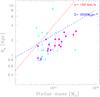 |
Fig. 1 Distribution of the ETGs of the total high-z sample in the Re − M⋆ plane (magenta points). Cyan triangles are a complete sample of ETGs selected from the GOODS-South field in the redshift range 1.2 <z< 1.6 (Tamburri et al. 2014) for reference. Blue(red) lines indicate lines of constant Σ(σ). We note that the sample of ETGs at ⟨ z ⟩ = 1.4 with velocity dispersions available is skewed toward more compact systems. |
3. IMF-σ trend as a function of time and mean stellar mass density
3.1. IMF-σ trend in local universe
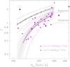 |
Fig. 2 Trend of Γ parameter (see Eq. (1)) as a function of velocity dispersion, for normal (mean stellar mass density Σ < 2500M⊙ pc-2) local ETGs (dark grey solid line) and for the whole local ETG population (long-dashed dark grey line). Dashed grey lines are the scatter around the best-fit relation of normal local ETGs, while grey open squares are the average values of the Γs of local normal ETGs in bin of ~50 km s-1. Magenta points are the upper limits of Γ we have derived for high-z ETGs in our spectroscopic sample at ⟨ z ⟩ = 1.4, and magenta solid line is their best-fit relation (magenta dashed lines indicate the rms around the relation). The black small-dotted lines are the best-fit relations of 100 subsamples of local ETGs, randomly extracted from the local sample by Tortora et al. (2013), in order to have the same Σandσe distribution of our spectroscopic sample at ⟨ z ⟩ = 1.4 (filled dark grey squares are an example of one local subsample). In this procedure we excluded three galaxies of the high-z sample (identified with magenta points with a black contour) since the local sample is missing ETGs with similar Σ and σe. The black point indicates the typical error on Γs of our spectroscopic sample at ⟨ z ⟩ = 1.4. |
Local studies have shown that IMF in spheroidal galaxies varies with their velocity dispersions. These studies compare the stellar mass-to-light ratio M/L⋆,ref derived through, e.g. the fit of the spectral energy distribution assuming a fixed reference IMF, with the true stellar mass-to-light ratio M/L⋆,true, derived through either dynamical models or spectral features analysis, and investigate how their ratio Γ = (M/L)⋆,true/ (M/L)⋆,ref varies with the physical properties of local ETGs.
Usually, this IMF-σ trend is presented in a form similar to ![Mathematical equation: \begin{equation} \log \Gamma = \log [(M/L)_{\star,{\rm true}}/(M/L)_{\star,{\rm ref}}] = \alpha \log \sigma_{\rm e} + \beta. \label{gamma} \end{equation}](/articles/aa/full_html/2015/01/aa24235-14/aa24235-14-eq81.png) (1)For the purpose of our analysis, as an example of Γ – σe trend in local ETGs, we have derived from the dataset of Tortora et al. (2013) the best-fit relation of Γ with σe for normal (Σ ≤ 2500 M⊙ pc-2) local ETGs with stellar mass and velocity dispersion comparable to that of our high-z sample (i.e. LogM⋆> 10.64 and σe ≳ 110 km s-1; we have already stated in the Introduction that all the trends found in local Universe are similar). Specifically, Tortora et al. (2013) derived, assuming different dark matter (DM) profiles, the Γ values for ~4500 giant ETGs drawn from the SPIDER project (La Barbera et al. 2010) in the redshift range of z = 0.05−0.1. The SPIDER sample is 95% complete at a stellar mass M⋆ = 3 × 10¹⁰M⊙, which corresponds to σ ~ 160 km s-1. In Fig. 2 we have reported the trend found assuming in the derivation of Γ a Navarro, Frenk and White profile (NFW, Navarro et al. 1996) for the DM component. Clearly, the effect of reducing the DM fraction is to increase the overall stellar mass normalization (for a clear picture of the effect of the degree of contraction on mass normalization see Dutton et al. 2011). In this figure, ETGs with Γ = 1 have true stellar masses in agreement with those derived with the reference IMF, in this case the one by Chabrier, while ETGs with Γ > 1 have stellar masses greater than that inferred with the Chabrier IMF, i.e. their IMF normalization is more massive.
(1)For the purpose of our analysis, as an example of Γ – σe trend in local ETGs, we have derived from the dataset of Tortora et al. (2013) the best-fit relation of Γ with σe for normal (Σ ≤ 2500 M⊙ pc-2) local ETGs with stellar mass and velocity dispersion comparable to that of our high-z sample (i.e. LogM⋆> 10.64 and σe ≳ 110 km s-1; we have already stated in the Introduction that all the trends found in local Universe are similar). Specifically, Tortora et al. (2013) derived, assuming different dark matter (DM) profiles, the Γ values for ~4500 giant ETGs drawn from the SPIDER project (La Barbera et al. 2010) in the redshift range of z = 0.05−0.1. The SPIDER sample is 95% complete at a stellar mass M⋆ = 3 × 10¹⁰M⊙, which corresponds to σ ~ 160 km s-1. In Fig. 2 we have reported the trend found assuming in the derivation of Γ a Navarro, Frenk and White profile (NFW, Navarro et al. 1996) for the DM component. Clearly, the effect of reducing the DM fraction is to increase the overall stellar mass normalization (for a clear picture of the effect of the degree of contraction on mass normalization see Dutton et al. 2011). In this figure, ETGs with Γ = 1 have true stellar masses in agreement with those derived with the reference IMF, in this case the one by Chabrier, while ETGs with Γ > 1 have stellar masses greater than that inferred with the Chabrier IMF, i.e. their IMF normalization is more massive.
3.2. IMF-σ trend for dense ETGs at ⟨ z ⟩ = 1.4
Following the same procedure adopted in the local Universe we have investigated the IMF-σe trend for the dense ETGs in our sample at ⟨ z ⟩ = 1.4.
After defining Mtot the total mass of the galaxy, and M⋆,ref the stellar mass given in Table 1, we derived the upper limit of the Γ parameter for the ETGs in our sample as Γ = Mtot/M⋆,ref. Assuming the total mass to be a proxy of the true stellar, we have implicitly assumed that these systems have zero DM.
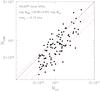 |
Fig. 3 Dynamical mass derived with 2D axisymmetric models, MJAM, versus virial mass, Mvir, derived as in Eq. (2) for the ETGs of the local ATLAS3D sample. MJAM was derived as stated in Cappellari et al. (2013b) in the caption of their Table 1. Although, on average, Eq. (2) overestimates the dynamical masses (black solid line is the 1:1 correlation), the offset (~0.2 dex) is not mass dependent. |
An important step in our analysis consists in deriving reliable total masses for ETGs in our sample. We addressed this point adopting the virial mass estimator, so for each galaxy in the sample 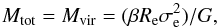 (2)where G is the gravitational constant and β is equal to
  (3)following Cappellari et al. (2006).
Typical errors on our Γ estimates are ~0.5. Detailed estimates of dynamical masses based on more sophisticated 2D axisymmetric dynamical models of local ETGs have shown that the virial Eq. (2) could overestimate the total masses (Cappellari et al. 2013b). In addition to the uncertainties on the true value of virial mass for each ETG, to which we will return later, we point out that the relative values of Mvir are not expected to change. In Fig. 3, the total dynamical mass of local ATLAS3D ETGs (Cappellari et al. 2011) derived with accurate 2D axisymmetric models (MJAM) is given versus their virial mass Mvir derived as in Eq. (2). The two mass estimates were derived from the ATLAS3D database as follows. The MJAM masses, following Cappellari et al. (2013b) (see caption of their Table 1), were derived as (M/L)JAM × L, where (M/L)JAM and L are the mass-to-light ratio obtained via dynamical models and the galaxy total luminosity, found in Cols. 6 and 15 of their Table 1, respectively. For the estimate of Mvir for ATLAS3D ETGs, we adopted for Re and n those derived from the 1D Sersic fit of the observed light profiles of the galaxy (Re,1D and n1D, Cols. 3 and 4 of the Table C.1 in Krajnović et al. 2013). Although the procedure they adopted to derive the Re is different from the 2D approach of GALFIT, the authors show that, at least for the Sersic index, the two procedures return similar results, with a difference of just 0.08 between the median values of the two distributions. For what concerns the σ, we referred to the stellar velocity dispersion measured by co-adding all SAURON spectra contained within the physical region of 1 kpc (Col. 4 of Table 1 in Cappellari et al. 2013b). We corrected this measure to those within Re,1D following Cappellari et al. (2006). In Fig. 3 we plot the ATLAS3D ETGs with 10.7 ≲ LogMvir ≲ 11.5 in order to approximately match the mass range of our spectroscopic sample. In this mass range, on average, we observe that Eq. (2) overestimates the dynamical masses, but the offset (~0.2 dex) is not mass dependent. The values of virial mass estimated via Eq. (2), therefore, are relatively reliable and hence, so are the Γ parameters of our high-z ETGs. Based on these considerations, and looking at the distribution of high-z dense ETGs in the Γ-σe plane, the first result we have found is that the Γ of high redshift dense ETGs show a trend with their σe (Spearman’s rank coefficient 0.84, probability 6.9 × 10⁻⁵) and that this trend is very similar to that observed in the local Universe, that is, their IMF becomes more massive with increasing velocity dispersion. In particular, in the range of velocity dispersion ~[120−300] km s-1 we have found Γ = 2.99 Logσe − 5.22 with a scatter of 0.28.
The possible uncertainties on the true value of Mvir do not affect this result, since the trend is dependent on relative values. Thus, within the approximation of our analysis, the trend of IMF with σe is also observed in high-z ETGs.
The second aspect we want to investigate is whether the IMF of ETGs depends on redshift and/or on mean stellar mass density. To address this second question we have compared the normalization of the IMF-σe trend we have found for dense ETGs at z ~ 1.4 with that observed in local universe.
Although we are making the extreme assumption of no dark matter, and thus the Γ we have derived for high-z ETGs are upper limits, the normalization of the IMF-σe trend for dense high-z ETGs is at 1σ lower than that observed for normal local ETGs. In particular, on average, at fixed velocity dispersion, the Γs of high-z dense ETGs are a factor of ~2 lower than the average value observed for normal local ETGs1. This could be ascribed to an evolution of IMF with redshift or to a dependence of IMF on mean stellar mass density. To discriminate between the two possibilities, we have compared the IMF-σe trend of high-z dense ETGs with that of equally dense local ETGs. In fact, if the IMF of massive dense ETGs depends on redshift, we should note that the average IMF-σe trend of local dense ETGs differ from the one we observe at high-z. Specifically, to address the topic, we randomly extracted from the sample of Tortora et al. (2013), 100 subsamples of local ETGs with Log[M⋆/M⊙] > 10.64 (as the high-z sample) and the same distribution in Σ and σe of our spectroscopic high-z sample. We checked the goodness of the local subsamples in reproducing the high-z sample with a KS test. In the random extraction, we retained a local subsample if the probability that its distribution of Σ and σe and that of the high-z sample are extracted from the same parent distribution is higher that 60%. In this procedure we excluded three galaxies of the high-z sample since the local sample is missing ETGs with similar Σ and σe. For each of these 100 subsamples we derived the best fitting Γ-σ relation in the range ~[120−300] km s-1. The resulting relations are shown in Fig. 2. Actually, the comparison shows that the IMF trend of dense high-z ETGs is consistent with that of local ETGs with similar velocity dispersion and mean stellar mass density.
However, we notice that our estimates of Γ are based on two assumptions, namely that on the DM and on the Eq. (2) as a reliable estimator of total mass. Although these assumptions do not affect the relative values of total masses (as we have shown above), they could have a significant impact on their absolute values, and hence on the normalization of the IMF-σe trend we observe. With regard to our assumption of zero dark matter fraction, we note that dense ETGs are expected to be stellar matter dominated (e.g. Conroy et al. 2013), and, on average, the dark matter fraction within the effective radius in massive dense local ETGs is found to be <10% (Tortora, priv. comm.). Similar results are derived also from ATLAS3D survey. Specifically, we checked the dark matter fraction fDM of ATLAS3D ETGs (taken form Cappellari et al. 2013a) with 10.7 ≲ LogMvir ≲ 11.5 and Σ > 2500 M⊙ pc-2 (for a detailed description of Σ estimates for ATLAS3D ETGs see below) and found that fDM = 0.11 ± 0.11. Moreover, simulations of dissipationless mergers of spheroidal galaxies have shown that this fraction can only decrease going back with time, pointing toward an even lower fraction of dark matter in high-z spheroidal galaxies (Hilz et al. 2013).
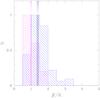 |
Fig. 4 Distribution of the ratio β/K for ATLAS3D ETGs with Σ ≥ 2500M⊙ pc2 (magenta histogram) and for those with Σ < 2500 M⊙ pc2 (blue histogram). Coloured solid lines are the median values of the two relative distributions, while black one refers to the total sample. We have included in the plot only local ETGs with stellar masses in the same range of dense high-z ETGs in our sample (10.7 ≲ LogMvir/M⊙ ≲ 11.5). The β parameter was derived through Eq. (3), while the K coefficient through Eq. (4). |
However, the values of Γ we have found for high-z systems could be affected by our uncertainties on true values of Mtot, hence of Mvir. In the following using the results obtained through 2D dynamical models of local ATLAS3D ETGs we show that Eq. (2) provides reliable absolute estimates of total masses for dense ETGs at z ~ 1.4. Cappellari et al. (2013b) in their Figs. 13 and 14, by comparing the estimates of total mass of local ETGs derived through accurate 2D dynamical models (MJAM) with those inferred from Eq. (2), clearly showed that the reliability of total masses estimated using the virial theorem is closely related to the choice of virial coefficient β and to the accuracy of Re estimates, which depends on the quality of the data and on the technique adopted to derive them. Following a similar approach, analogous results have been found by Shetty & Cappellari (2014) for massive galaxies at z ~ 1. As far as the robustness of size measurements of high-z ETGs, many works (e.g. Szomoru et al. 2012; Davari et al. 2014) have addressed the topic, showing that the typical approach adopted at high-z, i.e. 2D Sersic-fit of the light profile out to infinity on deep space-based images, is able to provide accurate Re estimates (uncertainties of ~15%). In the case in which radii are derived through this approach (i.e. through a Sersic-fit of the light profile out to infinity), Cappellari et al. (2013b) showed that the best approximation of dynamical masses is recovered assuming in the virial equation the non-homologous β coefficient of Eq. (3) rather than a constant virial coefficient (see the two right panels in their Fig. 14). Actually, in these conditions, Mvir shows systematic offset of ~0.2 dex with MJAM with a scatter 0.15 dex as we have shown in Fig. 3. To further exploit the origin of this offset we compared for ATLAS3D ETGs the value of their β coefficient, derived following Eq. (3), with those inferred from their 2D-dynamical models (K) as  (4)where MJAM was derived as described above, Re is Re,1D (Table C.1 from Krajnović et al. 2013) and σe is the velocity dispersion within 1 kpc (Table 1 Cappellari et al. 2013b) corrected to the Re,1D aperture.
In Fig. 4 we plot the distribution of the ratio β/K for ATLAS3D ETGs with Σ ≥ 2500M⊙ pc2 and for those with Σ < 2500 M⊙ pc2. To estimate the mean stellar mass density of ATLAS3D ETGs we adopted for Re the Re,1D values and derived their stellar masses multiplying the stellar mass-to-light ratio (Table 1 from Cappellari et al. 2013b) by the total luminosity L (Table 1 from Cappellari et al. 2013b). Since the ATLAS3D stellar mass-to-light ratio refers to the Salpeter IMF, we converted the stellar masses to the Chabrier IMF following Longhetti & Saracco (2009).
We have included in the plot of Fig. 4 only local ETGs with 10.7 ≲ LogMvir/M⊙ ≲ 11.5. Although, on average, for the total sample the β coefficient overestimates the virial masses of a factor ~1.35, this is principally due to normal ETGs (i.e. ETGs with Σ < 2500 M⊙ pc2). In fact, a clear trend of the β parameter with the compactness of the system emerges: while the majority of normal ETGs shows a β/K ratio >1 (median value 1.42 , where errors indicates the 25th and 75th percentile), for dense ETGs (~20 ETGs on a total of 103 ETGs in the figure) the virial masses estimated by means of Eq. (2) are perfectly in agreement with those inferred through more sophisticated dynamical models (median value of β/
 ). This result could be expected given the emerging picture on the variation of ETGs structure in the Re − M⋆ plane. Actually, Cappellari et al. (2013a) in their schematic summary of Fig. 14 clearly showed that in the mass range 3 × 10¹⁰<M⋆< 2 × 10¹¹ ETGs are dominated by the fast rotators, with very few slow rotators. However, at fixed stellar mass, the relevance of the bulge steadily increases with the mean stellar mass density. We argue, therefore, that the assumption of spherical isotropic models in the derivation of the β coefficient could fit better for dense systems than for normal ETGs, as can be seen in Fig. 4. Clearly, this result could not be necessarily valid for high-z dense ETGs which could be structurally and dynamically different from local ones. However, it has been found that both the kinematical and structural properties of dense high-z ETGs are very similar to those of equally dense local ETGs, and their β parameters should be similar as well. (e.g. Saracco et al. 2014; Trujillo et al. 2014; Ferré-Mateu et al. 2012; van der Wel et al. 2012; Buitrago et al. 2013). In this context, very interestingly, the mean value of the β parameter we have derived for our dense high-z ETGs is 7.0 ± 1.7, and perfectly agrees with the mean value of massive ATLAS3D dense ETGs, 7.5 ± 1.7.
To conclude, we have found that dense high-z ETGs i) follow the same IMF-σ trend of local ETGs; ii) have a lower mass normalization with respect to the average IMF-σ trend of normal local ETGs population; and iii) their mass-normalization is consistent with that of local ETGs with similar velocity dispersion and mean stellar mass density. In fact, neither our assumption about the dark matter fraction or the estimate of dynamical masses through virial estimator affect this result. Our finding of a lower mass normalization for dense high-z ETGs is in agreement with the recent result obtained through lens modeling of a z = 1.62 compact (Re ≃ 1.3 kpc, and M⋆ ≃ 2 × 10¹¹M⊙) early-type gravitational lens galaxy (Wong et al. 2014). Although the constraints are broad, the authors have found that the stellar mass of this galaxy is more consistent with that derived with a Chabrier IMF than with a Salpeter IMF.
In term of stellar content, these findings imply that at fixed velocity dispersion and at any redshift, the IMF of dense ETGs has a higher ratio of high- to low-mass stars, with respect to the IMF of typical local ETGs. In particular, assuming that the IMF is modelled as a single power law dN/dm ∝ m−s in the range of stellar masses [0.1−100] M⊙, we found that its slope varies from s = ~ 1.5 for high-z dense ETGs with velocity dispersion ~150 km s-1 to s = 2.35 (hence the Salpeter) for ETGs with velocity dispersion ~300 km s-1.
4. The IMF in massive spheroidal galaxies: Does it depend on when or on how ETGs assembled their stellar mass?
The similarity between the IMF trend of high-z and low-z dense ETGs over 9 Gyr of evolution and their lower normalization with respect to that of a typical local ETG suggest that i) the IMF in massive dense ETGs does not depend on the epoch at which they accreted their stellar mass and that ii) the physical conditions responsible for the higher mean stellar mass density of dense ETGs, at any redshift, favour a mass spectrum of new stars with a higher ratio of high- to low-mass stars with respect to that of a normal local ETGs.
Our current knowledge of dense ETGs shows that the compactness of a spheroidal galaxy is closely related to its star-formation rate (SFR). Local studies have shown that the FP residuals of local ETGs are anticorrelated both with galaxy age (e.g. Forbes et al. 1998; Reda et al. 2005; Gargiulo et al. 2009; Graves et al. 2009) and with the α-element abundance ratio, α/Fe (e.g. Gargiulo et al. 2009; Graves et al. 2009) in trends whereby ETGs more compact than expected from the FP relation have stellar populations systematically older and with higher abundances than average. However, a multiple regression analysis of FP residuals showed that α/Fe is the driving parameter, since there is no age correlation with compactness at fixed α/Fe, but a very strong α/Fe correlation at fixed age (e.g. Gargiulo et al. 2009). It has been long realized that the stellar α/Fe ratio is a robust indicator of the timescale τ of the star formation (e.g. Tinsley 1980; Greggio & Renzini 1983; Matteucci 1996), with higher abundance for shorter timescale. Thus, local results show that the compactness of a spheroidal galaxy is not the imprint of when it had assembled its stellar mass, but mostly of how, and more specifically, of the duration of its mass assembly history.
These findings show that the higher the SFR at which a galaxy assembles its stellar mass, the higher its compactness. Recent hydrodynamical simulations have shown that, in a galaxy, star formation at a rate greater than few M⊙ yr-1 leads to an increase of the Jeans mass of the system (Narayanan & Davé 2012), and thus inhibits the formation of low-mass stars. This result agrees with our findings. With respect to normal ETGs, the higher SFR that caracherizes the formation of dense ETGs, independently of z, should lead to a lack of low-mass stars with the consequent increase in the ratio of high- to low-mass stars, as we observe.
To summarize, on the basis of our results we have shown that high-z dense ETGs follow the same IMF-σ trend of local dense ETGs. This implies that the IMF of massive dense ETGs do not depend on time. Independently of z, the observed lower mass-normalization is a characteristic of ETGs with higher mean stellar mass density. If this result is extendible to all ETGs, that is, if the mass normalization is linked to the mean stellar mass density of the galaxies, then, at any redshift, the IMF of massive ETGs will have a higher or lower ratio of high- to low-mass stars according to the peculiar physical conditions in which a galaxy assembled its stellar mass.
Starting from these results, coupled with the recent findings on normal and dense ETGs, in the following we discuss the implication that our findings can have on the evolution with time of the mean IMF of ETGs population. Recent evidence suggests that the first spheroids formed in the early Universe, were dense (e.g. Saracco et al. 2010; Cassata et al. 2013; van Dokkum & Conroy 2010). At later epochs, compact ETGs continued to appear, together with normal ETGs, at least down to z ~ 1. In fact, the first studies of the number density of dense and normal massive quiescent galaxies have shown that dense spheroids were numerically dominant at z> 1 while normal ETGs are more common at z< 1 (Cassata et al. 2013). If the mass normalization of IMF is related to the mean stellar mass density, with densest systems those with a lower mass-normalization as we have found, the evolution of number density of dense and normal ETGs should imply a trend of the average IMF of massive ETGs population with z, in the direction of a higher mass-normalization with decreasing redshift. On this basis, consistent with the many theoretical predictions on the evolution of Jeans mass with redshift (see Introduction), our result implicitly suggests that the mean IMF of ETGs population in the early universe had a higher abundance of high-mass stars than the mean IMF of local ETG (assuming a power-law IMF). Clearly, this proposed picture needs to be further constrained by observations aimed at investigating the IMF in complete sample of massive ETGs at different epochs.
5. Summary and conclusions
We have used a spectroscopic sample of dense (Σ > 2500 M⊙ pc-2) ETGs we collected at z = 1.4 to investigate the variation of the IMF of massive ETGs as a function both of Σ and z. The results of our analysis are the following:
-
Massive dense ETGs at z = 1.4 follow the same IMF-σe trend of typicallocal ETGs, but with a lower mass-normalization. If massivedense ETGs were the first spheroids to form, as recent findingssuggest, this result shows that the average normalization of theIMF of the first massive ETGs is lower than that of a Chabrier IMF.This lower normalization could be an evidence of an evolution ofthe IMF with time or of a correlation with Σ
-
We find that the IMF-σe trend of dense ETGs at z = 1.4 is consistent with those of local ETGs with similar velocity dispersion and mean stellar mass density. This result is an evidence that the IMF, at least for dense ETGs, is not time dependent.
Irrespective of the formation redshift, at fixed velocity dispersion, the physical conditions which characterized the formation of dense ETGs lead to a mass spectrum of newly formed stars with a higher ratio of high- to low-mass stars than the IMF of typical ETGs of similar velocity dispersion. In facts, hydrodynamical simulations have shown that the Jeans Mass increases with the star-formation rate (SFR). Thus, given the higher SFR that should characterize the early phases of star formation of dense ETGs, we suggest that the lower mass-normalization we observe in dense ETGs is the result of a lack of low-mass stars.
On this basis, we suggest that the choice of the proper IMF for an individual massive ETG is not dependent on the time at which it assembled its stellar mass, but mostly on the efficiency of its star formation, hence on Σ.
Since the Γ of a given galaxy increases for decreasing amount of dark matter in the model, it could be more intuitive to expect that the IMF-σe trend we have derived had a higher mass-normalization than that of typical local ETGs. However, by definition, the Γ of a galaxy is Γ = Mtrue/ where fDM is the galaxy dark matter fraction. Thus, if we consider two different galaxies with the same velocity dispersion σe, the values of their Γs are not simply related to their dark matter fractions, but also to their Mref/Re ratio, hence to their mean stellar mass density. Thus, the position occupied by a galaxy in the IMF-σ plane does not only depend on its fDM, but also on its Re/M⋆ ratio.
Acknowledgments
The authors warmly thank the referee for his/her helpful comments and suggestions, and C. Tortora for the scientific discussions and for providing us with local data. This work has received financial support from Prin-INAF 1.05.09.01.05 and is based on observations made with ESO Very Large Telescope under programme ID 085.A-0135A.
References
- Bastian, N., Covey, K. R., & Meyer, M. R. 2010, ARAA, 48, 339 [Google Scholar]
- Bate, M. R. 2005, MNRAS, 363, 363 [NASA ADS] [Google Scholar]
- Bate, M. R., & Bonnell, I. A. 2005, MNRAS, 356, 1201 [NASA ADS] [CrossRef] [Google Scholar]
- Belli, S., Newman, A. B., & Ellis, R. S. 2014, ApJ, 783, 117 [NASA ADS] [CrossRef] [Google Scholar]
- Bezanson, R., van Dokkum, P., van de Sande, J., Franx, M., & Kriek, M. 2013, ApJ, 764, L8 [NASA ADS] [CrossRef] [Google Scholar]
- Bonnell, I. A., Clarke, C. J., & Bate, M. R. 2006, MNRAS, 368, 1296 [NASA ADS] [CrossRef] [Google Scholar]
- Bruzual, G., & Charlot, S. 2003, MNRAS, 344, 1000 [NASA ADS] [CrossRef] [Google Scholar]
- Buitrago, F., Trujillo, I., Conselice, C. J., & Häußler, B. 2013, MNRAS, 428, 1460 [NASA ADS] [CrossRef] [Google Scholar]
- Cappellari, M., & Emsellem, E. 2004, PASP, 116, 138 [NASA ADS] [CrossRef] [Google Scholar]
- Cappellari, M., Bacon, R., Bureau, M., et al. 2006, MNRAS, 366, 1126 [NASA ADS] [CrossRef] [Google Scholar]
- Cappellari, M., di Serego Alighieri, S., Cimatti, A., et al. 2009, ApJ, 704, L34 [NASA ADS] [CrossRef] [Google Scholar]
- Cappellari, M., Emsellem, E., Krajnović, D., et al. 2011, MNRAS, 413, 813 [NASA ADS] [CrossRef] [Google Scholar]
- Cappellari, M., McDermid, R. M., Alatalo, K., et al. 2012, Nature, 484, 485 [NASA ADS] [CrossRef] [Google Scholar]
- Cappellari, M., McDermid, R. M., Alatalo, K., et al. 2013a, MNRAS, 432, 1862 [NASA ADS] [CrossRef] [Google Scholar]
- Cappellari, M., Scott, N., Alatalo, K., et al. 2013b, MNRAS, 432, 1709 [NASA ADS] [CrossRef] [Google Scholar]
- Cassata, P., Giavalisco, M., Guo, Y., et al. 2011, ApJ, 743, 96 [NASA ADS] [CrossRef] [Google Scholar]
- Cassata, P., Giavalisco, M., Williams, C. C., et al. 2013, ApJ, 775, 106 [NASA ADS] [CrossRef] [Google Scholar]
- Chabrier, G. 2003, PASP, 115, 763 [NASA ADS] [CrossRef] [Google Scholar]
- Choi, J., Conroy, C., Moustakas, J., et al. 2014, ApJ, 792, 95 [NASA ADS] [CrossRef] [Google Scholar]
- Cimatti, A., Cassata, P., Pozzetti, L., et al. 2008, AA, 482, 21 [Google Scholar]
- Conroy, C., & van Dokkum, P. G. 2012, ApJ, 760, 71 [NASA ADS] [CrossRef] [Google Scholar]
- Conroy, C., Dutton, A. A., Graves, G. J., Mendel, J. T., & van Dokkum, P. G. 2013, ApJ, 776, L26 [NASA ADS] [CrossRef] [Google Scholar]
- Dabringhausen, J., Hilker, M., & Kroupa, P. 2008, MNRAS, 386, 864 [NASA ADS] [CrossRef] [Google Scholar]
- Dabringhausen, J., Fellhauer, M., & Kroupa, P. 2010, MNRAS, 403, 1054 [Google Scholar]
- Dabringhausen, J., Kroupa, P., Pflamm-Altenburg, J., & Mieske, S. 2012, ApJ, 747, 72 [NASA ADS] [CrossRef] [Google Scholar]
- Davari, R., Ho, L. C., Peng, C. Y., & Huang, S. 2014, ApJ, 787, 69 [NASA ADS] [CrossRef] [Google Scholar]
- di Serego Alighieri, S., Vernet, J., Cimatti, A., et al. 2005, A&A, 442, 125 [NASA ADS] [CrossRef] [EDP Sciences] [Google Scholar]
- Dutton, A. A., Conroy, C., van den Bosch, F. C., et al. 2011, MNRAS, 416, 322 [NASA ADS] [Google Scholar]
- Ferré-Mateu, A., Vazdekis, A., Trujillo, I., et al. 2012, MNRAS, 423, 632 [NASA ADS] [CrossRef] [Google Scholar]
- Ferreras, I., La Barbera, F., de la Rosa, I. G., et al. 2013, MNRAS, 429, L15 [NASA ADS] [CrossRef] [Google Scholar]
- Forbes, D. A., Ponman, T. J., & Brown, R. J. N. 1998, ApJ, 508, L43 [NASA ADS] [CrossRef] [Google Scholar]
- Gargiulo, A., Haines, C. P., Merluzzi, P., et al. 2009, MNRAS, 397, 75 [NASA ADS] [CrossRef] [Google Scholar]
- Gargiulo, A., Saracco, P., & Longhetti, M. 2011, MNRAS, 412, 1804 [NASA ADS] [CrossRef] [Google Scholar]
- Gargiulo, A., Saracco, P., Longhetti, M., La Barbera, F., & Tamburri, S. 2012, MNRAS, 425, 2698 [NASA ADS] [CrossRef] [Google Scholar]
- Gargiulo, A., Saracco, P., Longhetti, M., et al. 2014, A&A, submitted [Google Scholar]
- Graves, G. J., Faber, S. M., & Schiavon, R. P. 2009, ApJ, 698, 1590 [NASA ADS] [CrossRef] [Google Scholar]
- Grazian, A., Fontana, A., de Santis, C., et al. 2006, A&A, 449, 951 [NASA ADS] [CrossRef] [EDP Sciences] [Google Scholar]
- Greggio, L., & Renzini, A. 1983, A&A, 118, 217 [NASA ADS] [Google Scholar]
- Guo, Y., Giavalisco, M., Cassata, P., et al. 2011, ApJ, 735, 18 [NASA ADS] [CrossRef] [Google Scholar]
- Hennebelle, P., & Chabrier, G. 2008, ApJ, 684, 395 [NASA ADS] [CrossRef] [Google Scholar]
- Hilz, M., Naab, T., & Ostriker, J. P. 2013, MNRAS, 429, 2924 [NASA ADS] [CrossRef] [Google Scholar]
- Hopkins, P. F. 2013, MNRAS, 433, 170 [NASA ADS] [CrossRef] [Google Scholar]
- Ilbert, O., Salvato, M., Le Floc’h, E., et al. 2010, ApJ, 709, 644 [NASA ADS] [CrossRef] [Google Scholar]
- Ilbert, O., McCracken, H. J., Le Fèvre, O., et al. 2013, A&A, 556, A55 [NASA ADS] [CrossRef] [EDP Sciences] [Google Scholar]
- Jørgensen, I., & Chiboucas, K. 2013, AJ, 145, 77 [NASA ADS] [CrossRef] [Google Scholar]
- Krajnović, D., Alatalo, K., Blitz, L., et al. 2013, MNRAS, 432, 1768 [NASA ADS] [CrossRef] [Google Scholar]
- Kroupa, P. 2001, MNRAS, 322, 231 [NASA ADS] [CrossRef] [Google Scholar]
- Kroupa, P., Weidner, C., Pflamm-Altenburg, J., et al. 2013, The Stellar and Sub-Stellar Initial Mass Function of Simple and Composite Populations, eds. T. D. Oswalt & G. Gilmore, 115 [Google Scholar]
- La Barbera, F., de Carvalho, R. R., de La Rosa, I. G., et al. 2010, MNRAS, 408, 1313 [NASA ADS] [CrossRef] [Google Scholar]
- La Barbera, F., Ferreras, I., Vazdekis, A., et al. 2013, MNRAS, 433, 3017 [NASA ADS] [CrossRef] [Google Scholar]
- Larson, R. B. 1998, MNRAS, 301, 569 [NASA ADS] [CrossRef] [Google Scholar]
- Larson, R. B. 2005, MNRAS, 359, 211 [NASA ADS] [CrossRef] [Google Scholar]
- Läsker, R., van den Bosch, R. C. E., van de Ven, G., et al. 2013, MNRAS, 434, L31 [NASA ADS] [CrossRef] [Google Scholar]
- Longhetti, M., & Saracco, P. 2009, MNRAS, 394, 774 [NASA ADS] [CrossRef] [Google Scholar]
- Longhetti, M., Saracco, P., Severgnini, P., et al. 2007, MNRAS, 374, 614 [NASA ADS] [CrossRef] [Google Scholar]
- Longhetti, M., Saracco, P., Gargiulo, A., Tamburri, S., & Lonoce, I. 2014, MNRAS, 439, 3962 [NASA ADS] [CrossRef] [Google Scholar]
- Marks, M., Kroupa, P., Dabringhausen, J., & Pawlowski, M. S. 2012, MNRAS, 422, 2246 [NASA ADS] [CrossRef] [Google Scholar]
- Matteucci, F. 1996, Fund. Cosm. Phys., 17, 283 [Google Scholar]
- Munari, U., Sordo, R., Castelli, F., & Zwitter, T., 2005, A&A, 442, 1127 [NASA ADS] [CrossRef] [EDP Sciences] [Google Scholar]
- Narayanan, D., & Davé, R. 2012, MNRAS, 423, 3601 [NASA ADS] [CrossRef] [Google Scholar]
- Navarro, J. F., Frenk, C. S., & White, S. D. M. 1996, ApJ, 462, 563 [NASA ADS] [CrossRef] [Google Scholar]
- Padoan, P., & Nordlund, Å. 2002, ApJ, 576, 870 [Google Scholar]
- Papadopoulos, P. P. 2010, ApJ, 720, 226 [NASA ADS] [CrossRef] [Google Scholar]
- Papadopoulos, P. P., Thi, W.-F., Miniati, F., & Viti, S. 2011, MNRAS, 414, 1705 [NASA ADS] [CrossRef] [Google Scholar]
- Peng, C. Y., Ho, L. C., Impey, C. D., & Rix, H. 2002, AJ, 124, 266 [NASA ADS] [CrossRef] [Google Scholar]
- Reda, F. M., Forbes, D. A., & Hau, G. K. T. 2005, MNRAS, 360, 693 [NASA ADS] [CrossRef] [Google Scholar]
- Salpeter, E. E. 1955, ApJ, 121, 161 [Google Scholar]
- Santini, P., Fontana, A., Grazian, A., et al. 2009, A&A, 504, 751 [NASA ADS] [CrossRef] [EDP Sciences] [Google Scholar]
- Saracco, P., Longhetti, M., & Andreon, S. 2009, MNRAS, 392, 718 [NASA ADS] [CrossRef] [Google Scholar]
- Saracco, P., Longhetti, M., & Gargiulo, A. 2010, MNRAS, L115 [Google Scholar]
- Saracco, P., Casati, A., Gargiulo, A., et al. 2014, A&A, 567, A94 [NASA ADS] [CrossRef] [EDP Sciences] [Google Scholar]
- Shetty, S., & Cappellari, M. 2014, ApJ, 786, L10 [NASA ADS] [CrossRef] [Google Scholar]
- Smith, R. J. 2014, MNRAS, 443, L69 [NASA ADS] [CrossRef] [Google Scholar]
- Smith, R. J., & Lucey, J. R. 2013, MNRAS, 434, 1964 [NASA ADS] [CrossRef] [Google Scholar]
- Spiniello, C., Trager, S. C., Koopmans, L. V. E., & Chen, Y. P. 2012, ApJ, 753, L32 [NASA ADS] [CrossRef] [Google Scholar]
- Szomoru, D., Franx, M., Bouwens, R. J., et al. 2011, ApJ, 735, L22 [NASA ADS] [CrossRef] [Google Scholar]
- Szomoru, D., Franx, M., & van Dokkum, P. G. 2012, ApJ, 749, 121 [NASA ADS] [CrossRef] [Google Scholar]
- Tamburri, S., Saracco, P., Longhetti, M., et al. 2014, A&A, 570, A102 [NASA ADS] [CrossRef] [EDP Sciences] [Google Scholar]
- Tinsley, B. M. 1980, Fund. Cosm. Phys., 5, 287 [Google Scholar]
- Tortora, C., Romanowsky, A. J., & Napolitano, N. R. 2013, ApJ, 765, 8 [NASA ADS] [CrossRef] [Google Scholar]
- Treu, T., Auger, M. W., Koopmans, L. V. E., et al. 2010, ApJ, 709, 1195 [NASA ADS] [CrossRef] [Google Scholar]
- Trujillo, I., Ferré-Mateu, A., Balcells, M., Vazdekis, A., & Sánchez-Blázquez, P. 2014, ApJ, 780, L20 [NASA ADS] [CrossRef] [Google Scholar]
- van de Sande, J., Kriek, M., Franx, M., et al. 2013, ApJ, 771, 85 [NASA ADS] [CrossRef] [Google Scholar]
- van der Wel, A., Franx, M., van Dokkum, P. G., et al. 2005, ApJ, 631, 145 [NASA ADS] [CrossRef] [Google Scholar]
- van der Wel, A., Bell, E. F., Häussler, B., et al. 2012, ApJS, 203, 24 [NASA ADS] [CrossRef] [Google Scholar]
- van Dokkum, P. G., & Conroy, C. 2010, Nature, 468, 940 [NASA ADS] [CrossRef] [Google Scholar]
- Wong, K. C., Tran, K.-V. H., Suyu, S. H., et al. 2014, ApJ, 789, L31 [NASA ADS] [CrossRef] [Google Scholar]
All Tables
All Figures
|
Fig. 1 Distribution of the ETGs of the total high-z sample in the Re − M⋆ plane (magenta points). Cyan triangles are a complete sample of ETGs selected from the GOODS-South field in the redshift range 1.2 <z< 1.6 (Tamburri et al. 2014) for reference. Blue(red) lines indicate lines of constant Σ(σ). We note that the sample of ETGs at ⟨ z ⟩ = 1.4 with velocity dispersions available is skewed toward more compact systems. |
| In the text | |
|
Fig. 2 Trend of Γ parameter (see Eq. (1)) as a function of velocity dispersion, for normal (mean stellar mass density Σ < 2500M⊙ pc-2) local ETGs (dark grey solid line) and for the whole local ETG population (long-dashed dark grey line). Dashed grey lines are the scatter around the best-fit relation of normal local ETGs, while grey open squares are the average values of the Γs of local normal ETGs in bin of ~50 km s-1. Magenta points are the upper limits of Γ we have derived for high-z ETGs in our spectroscopic sample at ⟨ z ⟩ = 1.4, and magenta solid line is their best-fit relation (magenta dashed lines indicate the rms around the relation). The black small-dotted lines are the best-fit relations of 100 subsamples of local ETGs, randomly extracted from the local sample by Tortora et al. (2013), in order to have the same Σandσe distribution of our spectroscopic sample at ⟨ z ⟩ = 1.4 (filled dark grey squares are an example of one local subsample). In this procedure we excluded three galaxies of the high-z sample (identified with magenta points with a black contour) since the local sample is missing ETGs with similar Σ and σe. The black point indicates the typical error on Γs of our spectroscopic sample at ⟨ z ⟩ = 1.4. |
| In the text | |
|
Fig. 3 Dynamical mass derived with 2D axisymmetric models, MJAM, versus virial mass, Mvir, derived as in Eq. (2) for the ETGs of the local ATLAS3D sample. MJAM was derived as stated in Cappellari et al. (2013b) in the caption of their Table 1. Although, on average, Eq. (2) overestimates the dynamical masses (black solid line is the 1:1 correlation), the offset (~0.2 dex) is not mass dependent. |
| In the text | |
|
Fig. 4 Distribution of the ratio β/K for ATLAS3D ETGs with Σ ≥ 2500M⊙ pc2 (magenta histogram) and for those with Σ < 2500 M⊙ pc2 (blue histogram). Coloured solid lines are the median values of the two relative distributions, while black one refers to the total sample. We have included in the plot only local ETGs with stellar masses in the same range of dense high-z ETGs in our sample (10.7 ≲ LogMvir/M⊙ ≲ 11.5). The β parameter was derived through Eq. (3), while the K coefficient through Eq. (4). |
| In the text | |
Current usage metrics show cumulative count of Article Views (full-text article views including HTML views, PDF and ePub downloads, according to the available data) and Abstracts Views on Vision4Press platform.
Data correspond to usage on the plateform after 2015. The current usage metrics is available 48-96 hours after online publication and is updated daily on week days.
Initial download of the metrics may take a while.