| Issue |
A&A
Volume 573, January 2015
|
|
|---|---|---|
| Article Number | A4 | |
| Number of page(s) | 7 | |
| Section | The Sun | |
| DOI | https://doi.org/10.1051/0004-6361/201423385 | |
| Published online | 08 December 2014 | |
Alfvénic waves in polar spicules⋆
1
Institut d’Astrophysique de Paris, UMR 7095, CNRS and UPMC,
98Bis Bd. Arago,
75014
Paris,
France
e-mail:
This email address is being protected from spambots. You need JavaScript enabled to view it.
2
Physics Department, Payame Noor University (PNU),
19395-3697
Tehran,
Iran
3
Center for Excellence in Astronomy & Astrophysics
(CEAA), Research Institute for Astronomy & Astrophysics of Maragha
(RIAAM), PO Box,
55134-441
Maragha,
Iran
4
Department of Physics, Tabriz Branch, Islamic Azad
University, Tabriz,
Iran
Received: 8 January 2014
Accepted: 25 September 2014
Abstract
Context. For investigating spicules from the photosphere to coronal heights, the new Hinode/SOT long series of high-resolution observations from space taken in CaII H line emission offers an improved way to look at their remarkable dynamical behavior using images free of seeing effects. They should be put in the context of the huge amount of already accumulated material from ground-based instruments, including high- resolution spectra of off-limb spicules.
Aims. Both the origin of the phenomenon and the significance of dynamical spicules for the heating above the top of the photosphere and the fuelling of the chromospheric and the transition region need more investigation, including of the possible role of the associated magnetic waves for the corona higher up.
Methods. We analyze in great detail the proper transverse motions of mature and tall polar region spicules for different heights, assuming that there might be Helical-Kink waves or Alfvénic waves propagating inside their multicomponent substructure, by interpreting the quasi-coherent behavior of all visible components presumably confined by a surrounding magnetic envelop. We concentrate the analysis on the taller CaII spicules more relevant for coronal heights and easier to measure. Two-dimensional velocity maps of proper motion were computed for the first time using a correlation tracking technique based on FFTs and cross-correlation function with a 2nd-order-accuracy Taylor expansion. Highly processed images with the popular mad-max algorithm were first prepared to perform this analysis. The locations of the peak of the cross-correlation function were obtained with subpixel accuracy.
Results. The surge-like behavior of solar polar region spicules supports the untwisting multicomponent interpretation of spicules exhibiting helical dynamics. Several tall spicules are found with (i) upward and downward flows that are similar at lower and middle levels, the rate of upward motion being slightly higher at high levels; (ii) the left- and righthand velocities are also increasing with height; (iii) a large number of multicomponent spicules show shearing motion of both left- and righthanded senses occurring simultaneously, which might be understood as twisting (or untwisting) threads. The number of turns depends on the overall diameter of the structure made of components and changes from at least one turn for the smallest structure to at most two or three turns for surge-like broad structures. The curvature along the spicule corresponds to a low turn number similar to a transverse kink mode oscillation along the threads.
Key words: Sun: chromosphere / Sun: transition region
A movie associated to Fig. 1 is available in electronic form at http://www.aanda.org
© ESO, 2014
1. Introduction
Spicules are jet-like chromospheric structures and are usually seen all around the limb of the Sun, see Tsiropoula et al. (2012) for a recent exhaustive review presentation with a rather conservative point of view and covers the ground-based observations well. As far as time sequences of images are concerned, ground-based observations of extremely fine off-limb spicules have suffered from the terrestrial turbulence effects. Spicules arise in different directions in the low-level interface between the photosphere and the corona. Their emission in low-excitation emission lines is responsible for the part of the interface usually called the chromospheric shell where HI, HeI, and HeII high first ionization potential (FIP) emission lines are seen and further out, toward the higher temperature transition region (TR) (see Bazin & Koutchmy 2013 for eclipse observations free of parasitic scattered light). Indeed, eclipse observations showed for a long time that at the lowest 4 Mm heights the temperature remains low (Matsuno & Hirayama 1988).
The mechanism of spicule formation and their evolution are not well understood (see the reviews by Sterling 2000; Zaqarashvili & Erdélyi 2009 and by Mathioudakis et al. 2013; for different propulsive mechanisms, see, e.g., Lorrain & Koutchmy 1996 and Lorrain & Koutchmy 1998; Filippov et al. 2007; and Tavabi et al. 2011a). The investigation of solar spicules is needed to understand the transition region and the chromosphere and possibly some aspect of coronal heating (Kudoh & Shibata 1999), especially in the case of tall or giant spicules that have more chance to contribute in the corona. The mature spicules are fairly homogeneous in height and have a lifetime of approximately 5−15 min, which is comparable to the photospheric granules lifetime. They have typical upflow speeds of 20−50 kms-1 and are sometimes much higher for giant spicules. Spicule diameters in the chromosphere range from 200 km to 500 km when individual components with shorter apparent lifetimes are considered. They are now often called type II spicules, starting with De Pontieu et al. (2007). Some objections regarding their significance were expressed (Zhang et al. 2012; Klimchuk 2012); a more detailed and documented description was also given based on excellent ground-based SST spectroscopic observations and analysis (De Pontieu et al. 2012) that we found agrees with much earlier results by Dara et al. (1998). Indeed, type II spicules were also discussed in the framework of macro-spicules and even blow-out SXR coronal jets by Sterling et al. (2010a,b), confirming that they are the components of a more significant event.
Following the results of our statistical and morphological analysis of spicules (Tavabi et al. 2011a, 2012, 2013), we will not really distinguish type II spicules from the larger structure they are a part of. The corresponding unseen magnetic flux tube, envelope, or shell surrounding a set of spicule components is evidently larger than the spicule itself. They usually reach heights of typically 4 Mm and up to 10 Mm before fading out of view or fall free back toward the solar surface. Their smallest widths can be only 100−200 km, close to the resolution limit of the best telescopes. Tavabi et al. (2011a) found that spicules indeed show a whole range of diameters, including unresolved interacting spicules (I-S), depending on the definition chosen to characterize this ubiquitous dynamical phenomenon occurring inside a low TR and coronal background.
Spicules are very thin and numerous, so along the line of sight some overlapping could occur, especially near and above the limb where a long integration along the line of sight exists when the projection in the plane of the sky is considered. Superposition effects (overlapping) are more important than has previously been anticipated, when it was thought that spicules have at least 1 Mm or more diameter, because the number of spicules intercepted along the line of sight per resolution element is indeed considerable. A kind of collective and quasi-coherent behavior by two or more components of spicules was described for the first time in Tavabi et al. (2011a) and Tavabi (2014). Most spicules were found to have a multiple structure (similarly to the doublet spicules described in Suematsu et al. 1995 and Tsiropoula et al. 2012) and show impressive transverse periodic behavior, which was interpreted as upwardly propagating kink or Alfvén waves.
Spicules usually show an oscillatory behavior (Zaqarashvili & Erdélyi 2009). The existence of five-minute oscillations in spicules were originally reported by Nikolsky & Platova (1971), Kulidzanishvili & Nikolsky (1978), and others, including spectroscopically performed observations with a large aperture coronagraph. More recently, image sequences have been studied by De Pontieu et al. (2004), Xia et al. (2005), and Ajabshirizadeh et al. (2008). Oscillations in spicules with even shorter periods have been reported by Nikolsky & Platova (1971). They found that spicules oscillate along the limb with a characteristic period of about 1 min, a remarkable result confirmed by recent analysis of SOT (Hinode) spicules showing <120 s transverse oscillations from time-slice analysis (Tavabi et al. 2011a). Kukhianidze et al. (2006) report periodic spatial distribution of Doppler velocities with height through spectroscopic analysis of Hα series in solar limb spicules (at the heights of 3800−8700 km above the photosphere).
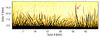 |
Fig. 1 Example of an image processed by the mad-max algorithm. The image is based on a Hinode/SOT narrowband Ca II H image taken on 17 June 2011 at 9:13:42.4 UT. The color table is inverted to produce a negative image. The arrow points to the long twisted spicule and the loop structures next to it. A movie showing the temporal evolution is available online. (The spinning motions in the movie are most obvious when the movie is manually run at a higher speed than the default speed.) |
Suematsu et al. (2008) report the observation of twist motion of spicules from Hinode/SOT image observations, and He et al. (2009) find high-frequency transverse motion in spicules, which also agrees with the results of Tavabi et al. (2011a). Additional statistically significant parameters should be determined to permit a full interpretation of the phenomenon, including a possible spinning motion. Rotation about the quasi-radial axis of spicules has been inferred in several early classical spectroscopic studies (e.g., Pasachoff et al. 1968) from the tilts observed on slit spectra, without fully resolving the components of spicules (Dara et al. 1998) and the suggestion of spinning and/or helical motion in emerged flux tubes is a recurrent suggestion by theoreticians considering the currents inside (e.g., Shibata & Uchida 1986) and by observers (e.g., Rompolt 1975).
2. Observations
We selected two sequences of solar limb observations in the polar region with the broad-band filter instrument (BFI) of the Hinode/SOT (Fig. 1). We used several series of image sequences obtained on 17 June 2011 (south sole) and 25 Oct. 2008 (north pole) in the Ca II H emission line, with the wavelength passband centered at 398.86 nm with an FWHM of 0.3 nm. A fixed cadence of 1.6 s (for 25 Oct. 2008 it is about 10 s) is used (with an exposure time of 0.5 s), giving a spatial resolution of the Hinode/SOT observations limited by the diffraction pattern to 0.16 arcsec (120 km); a 0.1 arcsec pixel size scale is used. The image size for 17 June 2011 is 512 × 512 pixels (readout performed only over the central pixels of the larger detector to keep the high cadence within the telemetry restrictions) that covers an area of (field of view, FOV hereafter) 55.78 × 55.78 arcsec2, and the images size is 512 × 1024 and FOV about of 55.78 × 111.57 arcsec2 for the 25 Oct. 2008 observations. On the polar cap of the Sun, spicules are somewhat more numerous than at low latitudes close to the solar equator, and they are slightly taller and definitely oriented more radially (Filippov & Koutchmy 2000). We used the SOT routine fg_prep to reduce the image spikes and jitter and to align the time series. The time series showed a slow instrumental drift, with an average speed smaller than 0.015 arcsec/min toward the north, as identified from solar limb motion.
The analysis is performed after the data are subjected to a deep processing for showing thread-like features. This is obtained using the mad-max algorithm (Koutchmy & Koutchmy 1989; Tavabi et al. 2012, 2013); see Fig. 1 for a sample. This spatial nonlinear filtering clearly shows rather bright radial threads in the chromosphere as fine as the resolution limit of about 120 km, without any doubt confirming the high quality of Hinode/SOT observations. It permits us to evaluate, in first-order approximation, what the properties of individual spicules could be. Unfortunately the signal-to-noise (S/N) level does not permit us to utilize the full spatio-temporal resolution, as illustrated in Fig. 2. Accordingly, we further restrict our analysis to the longest features, specifically the ones that can be automatically measured with a computer-aided algorithm, leaving the investigation of the ultimate very dynamical details seen in Fig. 2 for a future paper.
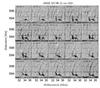 |
Fig. 2 Example of rapidly moving features observable at the ultimate SOT resolution, after using the mad-max processing and a negative image display of the results. Only the first 5 Mm heights above the limb are shown. |
3. Data analysis
Regarding the image processing, we found superior results after using a spatial image processing for both thread-like (or elongated) and loop-like features obtained with the so-called mad-max algorithm (Koutchmy & Koutchmy 1989). The mad-max operator acts to substantially enhance the finest scale structure. The mad-max operator is a weakly nonlinear modification of a second derivative spatial filter that improves the resolution limit near the Nyquist frequency where the S/N is evidently critical. Specifically, it is where the second derivative has a maximum when looking along different directions. (Usually, 8 directions around each pixel are used to make the image processing fast.)
The behavior of mad-max qualitatively resembles the second derivative, but the strong selection effect for the direction of the maximum variation substantially enhances the intensity modulations of the most significant structures and, accordingly, considerably reduces the noisy background usually appearing in high spatial filtering near the Nyquist frequency. It also appears to reduce the blending (due to overlapping effects) between crossing threads superposed along the line of sight. The algorithm, as originally proposed, samples the second derivative in eight directions, but the directional variation of the second derivative was generalized to a smooth function with a selectable passband spatial scale for this work (for more details see November & Koutchmy 1996 and the more recent paper by Tavabi et al. 2013). Spatial filtering using Mad-Max algorithms clearly shows relatively bright radial threads in the chromosphere as fine as the resolution limit of about 120 km (Fig. 1). Some deviation from the radial direction is observed, and the aspect ratio of each spicule is often greater than 10.
4. Results
The selected spicules show a peculiar structure as indicated in the Fig. 3 in the center. Only a small part of all spicules seen in the time series are shown, with a definite twisting effect and isolated enough to avoid superposition effects. Ten very long and obvious spicules in each time series were studied in detail, after selecting the features where the overlapping effect is less important and where spicules are somewhat taller (see the example shown in Fig. 1). We chose an axis close to the local vertical axis for each case, to follow the details with respect to this relative axis. Furthermore, we used the Fourier local correlation tracking algorithm (FLCT) to map the apparent proper motions over the FOV of each case. This is a powerful cross-correlation technique for measuring proper motions of tracers seen on successive frames of a time series of solar features. The original concept of the FLCT algorithm was published by November & Simon (1988), and later the algorithm was improved by Fisher & Welsch (2007). They describe the computational techniques for constructing a 2D velocity field that connects two successive images taken at two different times; one must start from some given location within both images, compute a velocity vector, and then repeat the calculation while varying that location over all pixel positions. The cross-correlation is defined as a function of position in the image, within a spatially localized apodization window by Gaussian function with a typical width. The distance between spatially localized cross-correlation maxima divided by the time interval gives a measure of the proper motion projected on the plane of the sky.
It works with two images separated in time and gives an estimate for a 2D velocity field by finding the shifts that increase a local cross-correlation function between the two images. Pixel size was 0.1 arcsec and matrices were shifted by the same value to compute crosss-correlations. Using the FLCT algorithm for each spicule-case, we then deduced a 2D velocity diagram as shown in Figs. 3−5. After evaluating all maps, we find that a high percentage of solar coronal hole spicules i/ show surge-like behavior (see Sect. 5 for a description of surge); and ii/ support an interpretation as twisting multicomponent spicules. The processed accompanying movie corresponding to the 17 June 2009 observations (6 min 45 s long with a 3 s cadence) offers more support for our results.
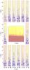 |
Fig. 3 Example obtained using the FLCT algorithm for showing the 2D velocity maps from successive frames with a corresponding remarkable structure shown by the red arrow over a larger FOV shown in negative at the center. Spatial units used in the display are 0.1 arcsec (corresponds to pixel size), and the cadence is 1.6 s. Intensities in the proper motion maps are reproduced in red-orange. Note the large magnification needed to clearly evaluate the results (see in better reproduction in the electronic color version, to be magnified); see Fig. 4 for a quantitative evaluation of the amplitudes of velocities. |
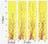 |
Fig. 4 Selected frames from the left top first row of the preceding Fig. 3. The scale of apparent velocities is shown at the bottom using a small black bar put over the typical value affected by an error of ±5 km s-1. |
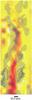 |
Fig. 5 Zoom of a small part of the preceding Fig. 3, bottom of the last frame, showing at the bottom the scale of apparent velocities measured using the FLCT algorithm at ultimate resolution. Pixel size is 0.1 arcsec and time cadence only 1.6 s. An artifact is produced outside the structures with arrows pointing upward. The method is not suitable for measuring proper motion when the velocity is aligned along an extended fine structure as in the case of a vertical, up or down, flow along a quasi-radial spicule. |
We detected several long spicules showing similar behavior and found that the upward and downward flows are equal for lower and middle levels (see Fig. 6), but the rate of upward motion is slightly higher in high levels. However, we cannot really trust the deduced values of up and down velocities because the FLCT algorithm used at the ultimate resolution is poorly responding to velocities directed along a fine structure, which is predominantly directed along the local radial direction (vertical). As suggested by Fig. 2, high amplitude velocities could exist. As far as the shearing motion in the left and right directions is concerned, it is also equal at all heights.
The features are difficult to measure precisely because the S/N is fairly marginal, and the variations are extremely fast. The frames are separated by only 3 s and the field covers just 5 × 5 Mm2. The neo-spicule feature (shown with a white inclined bar /) at 05:17:00 is rapidly rising vertically until 05:17:06 UT and then seems to slowly fall during at least the next six seconds. The second neo-spicule feature (shown with a white >) at 05:17:30 rises rapidly with a small angle to the vertical until 05:17:36, fades, and then rises at 05:17: 51 with some evidence of a twist 6 s later at 05:17:57 UT. The apparent associated upward velocities are typically 250 ± 100 km s-1 in both cases, when taking the scale (given in Mm) and the pixel size of 0.1 arcsec or 74 km in July into account. We note the bright low lying feature under the 694 Mm height that could be a small loop. The horizontal signature of an artifact of the CCD reading at the 694.7 Mm and the 696.1 Mm heights appear as noise that is difficult to remove.
In Fig. 6, velocity diagrams shown as orange strips at the top we are obtained using the FLCT algorithm used in the vertical (up and down) and horizontal (left and right) directions and the blue curves under each strip give the corresponding velocity values. Up and down velocities are probably underestimated because structures are predominantly aligned in the vertical direction.
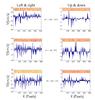 |
Fig. 6 Distribution of horizontal and vertical proper motion velocities for different layers or slices above the limb as given by the height H in arcsec above the surface (limb) as observed on 17 June 2011. The orange band at the top shows the area selected at different heights, and the plots show the dispersion around the mean values. |
Finally, we plotted histograms of velocities. We found the amplitudes are increasing with the height (Fig. 7) for the left- and righthand velocities. The analysis is repeated for another sequence with different images and data taken on 25 Oct. 2008.
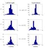 |
Fig. 7 Histograms for swaying and up and down motions for different heights observed on 17 June 2011. |
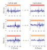 |
Fig. 8 Horizontal and vertical proper motion velocities for different layers above the limb as observed on 25 Oct. 2008. |
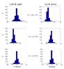 |
Fig. 9 Histograms for swaying and up and down motions for different heights on 25 Oct. 2008. |
5. Discussion
Generally speaking, a large number of multicomponent spicules have been observed. It immediately comes to mind that it maybe possibly comparable to surge-like events observed in polar regions, which are also called macro-spicules (e.g., Georgakilas et al. 2001). Because torsional motion occurs simultaneously and close to other components (Figs. 6 to 9), it might be interpreted as twisting threads, see Fig. 10 for a naive representation). According to the 2D image of a spicule, it is thought that the waves are kink mode, but according to the 3D display, wave propagation in a tube is seen as helical and kink, what we call helical-kink because the spicule axis is displaced. The number of twists depends on the diameter of the set of components with coherent behavior and changes from at least 1 turn for very thin structures to at most two or three turns for mini-surge-like, very broad structure. A curvature shape looking similar to a transverse kink-mode oscillation along the threads is possibly produced by a low twist number.
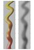 |
Fig. 10 Cartoon showing a twisted thread (at left) using a 3D effect with propagation of torsional motion, and in the right panel, the corresponding view in 2D assuming the plasma is optically thin at this emission line (shown in negative). |
Figure 1 shows an example of what could be long rotating and untwisting Macro-spicules. We suggest that such spicules have a multicomponent structure and are created by the disruption of a primary loop (Tavabi et al. 2011b). In the polar regions spicules are longer and less tilted (Tavabi et al. 2012), so the probability of observing individual spicules increases. Also, the lower density of the background in the polar regions helps us to see spicule footpoints better.
Surges are cool plasma jets ejected from small flare-like chromospheric bright points, including regions near the poles, such as subflares. Some similarity possibly exists with Ellerman bombs (moustaches) that usually appear near sunspots at lower latitudes. These cool plasma jets are a kind of active small prominence, usually observed in Hα at ground-based observatories (Georgakilas et al. 1999, 2001) and known for a long time from eclipse observations (e.g., Fig. 140, p. 389 in Secchi 1875), although space observations, such as with extreme-ultraviolet (EUV) telescopes, also detect surges. Surges in TR lines are ejected at peak velocities of 50–200 km s-1 along a straight or slightly curved path, delineating magnetic field lines. They reach heights of 10 000–100 000 km and typically last 10–20 min. Some of the surges show a spinning motion at a few tens of km s-1 around their axis, during the ejection phase, see the classical work of Rompolt (1975) for an exhaustive description of Hα coronagraphic observations.
The direction of spinning motion is consistent with the direction of unwinding motion of their helical twist. Small surges are then similar to twisty spicules, which are cool chromospheric jets observed in Hα and EUV at the network boundary. The velocity and height are about 30 to 250 km s-1 and 5000−8000 km at most, much less than those of surges, while the temperature and electron density are comparable to those of surges. Macro-spicules also show a velocity feature that suggests spinning motion (Georgakilas et al. 1999, 2001). Macrospicules are observed in coronal holes and show characteristic parameters between those of spicules and those of surges. They are ejected at velocities on the order of 140 km s-1, reaching heights of 10 000−35 000 km, and they show nearly ballistic motion (Tavabi et al. 2011b; Tsiropoula et al. 2012). Spinning motion can also be interpreted by taking reconnections between the twisted flux tube and the untwisted magnetic field of the background corona into account. Therefore it is very likely that magnetic reconnection is a key to producing surges as also suggested for coronal polar jet (Patsourakos et al. 2008). If a magnetic field line reconnects with another field line, a magnetic tension force is generated in the reconnected field line as in a slingshot (described in, e.g., Tavabi et al. 2011c). Such a magnetic tension force accelerates plasmas in the reconnected field line up to the Alfvén speed outside the current sheet.
We note that in case jet spicules are cool enough, it is difficult to accelerate such cool jets by gas pressure alone without raising the temperature, whereas it is quite easy to accelerate cool jets by magnetic force while keeping a low temperature. As a result, the magnetically driven jet mechanism would have a wider applicability as a model for both cool jets and for hot X-ray jets (Filippov et al. 2009). This is especially true for larger jets (such as large surges and sprays), although, becuase it is for smaller jets (such as spicules and small surges). A possibility remains that jets are accelerated by the gas pressure force of a slow-mode MHD shock.
The study of spinning spicules seems important for the following reasons:
-
a)
Because of conservation of the torsional magnetic fields, it cangive us information about the origin of spicules.
-
b)
Our work presented here and other studies using both filtergrams and limb spectra (Pasachoff et al. 1968; Nikolsky & Platova 1971; Tanaka 1974; Kulidzanishvili & Nikolsky 1978; Gadzhiev & Nikolsky 1982; Suematsu et al. 1995; Dara et al. 1998; Georgakilas et al. 1999 and recently in Tavabi et al. 2011a) clearly suggest that spicules are multicomponent. At each moment, we usually can only see just a part of it clearly; accordingly, the spatial and the temporal resolution should be better than the values of the diameter of each component and its lifetime. We should emphasize that the spinning motions of limb spicules have already been reported (Pasachoff et al. 1968; Georgakilas et al. 2001; Tavabi 2014) with the suggestion from time sequences of photographic limb spectra taken with the giant soviet era 52 cm aperture Lyot coronagraph that the spinning trajectory is elliptical (Gadzhiev & Nikolsky 1982). Spinning motion in erupting prominences can be studied more easily (Rompolt 1975).
-
c)
Propagation of Alfvénic waves in spicules and especially farther out along the magnetic field can be considered for heating the corona and for supplying the material for the solar wind.
To understand the origin of the twist of the loops, several scenarios have been presented; each of them attempts to explain the origin of this behavior using different assumptions. It seems that untwist results from a tearing of initially helically structured loops (Fig. 1). In these images a loop was seen at the feet of twisted spicules. Based on the conservation of rotational momentum (or helicities), we can expect that the expansion of chromospheric mini-loops finally leads to micro-eruptions similar to spicule eruption of the spine type (Tavabi et al. 2011c). To go further with observations, some better S/N high-resolution frames are needed (Fig. 2), which means larger aperture telescopic observations, as are now available with the NST at BBSO, and those planned with the ATST at Hawaii and with the future ISAS Solar C space telescope. Meanwhile, numerical simulations would help a lot, so we look forward to evaluating more simulations of the spicule phenomenon, starting from the surface of the Sun where granular and subgranular motions and possibly p-mode interactions in the presence of a background magnetic field of the chromopsheric network would produce helical small scale eruptions (Kitiashvili et al. 2013). The dissipation effects resulting from the local dynamo effects in converging flows (Lorrain & Koutchmy 1996, 1998) will also be taken into account.
Online material
Movie of Fig. 1 Access Supplementary Material
Acknowledgments
We are grateful to the Hinode team for their wonderful observations. Hinode is a Japanese mission developed and launched by ISAS/JAXA, with NAOJ as domestic partner and NASA, ESA, and STFC (UK) as international partners. Image processing software was provided by O. Koutchmy, see http://www.ann.jussieu.fr/~koutchmy/index_newE.html. The FLCT source code and compilation instructions were downloaded from http://solarmuri.ssl.berkeley.edu/overview/publicdownloads/software.html. This work has been supported by Research Institute for Astronomy & Astrophysics of Maragha (RIAAM) and the Center for International Scientific Studies & Collaboration (CISSC), by the French Embassy in Tehran and the French Institut d’Astrophysique de Paris–CNRS and UPMC. We thank Leon Golub for his careful reading of the draft and for meaningful suggestions and Alphonse Sterling for comments and suggestions. Last but not least, we thank the referee(s) and the editor for meaningful suggestions and requests that greatly improved the original draft.
References
- Ajabshirizadeh, A., Tavabi, E., & Koutchmy, S. 2008, New Astron., 13, 93 [NASA ADS] [CrossRef] [Google Scholar]
- Antolin, P., & Rouppe van der Voort, L. 2012, ApJ, 745, 152 [NASA ADS] [CrossRef] [Google Scholar]
- Bazin, C., & Koutchmy, S. 2013, J. Adv. Res, 4, 307 [CrossRef] [Google Scholar]
- Brooks, D. H., Warren, H. P., Ugarte-urra, I., & Winebarger, A. R. 2013, ApJ, 772, 19 [Google Scholar]
- Cirtain, J. W., Golub, L., Winebarger, A. R., et al. 2013, Nature, 493, 501 [NASA ADS] [CrossRef] [Google Scholar]
- Dara, H. C., Koutchmy, S., & Suematsu, Y. 1998, Properties of Hα Spicules from Disk and Limb High-Resolution Observations, Solar Jets and Coronal Plumes, ESA SP-421, 255 [Google Scholar]
- De Pontieu, B., Erdélyi, R., & James, S. P. 2004, Nature, 430, 536 [NASA ADS] [CrossRef] [PubMed] [Google Scholar]
- De Pontieu, B., McIntosh, S., Hansteen, V. H., et al. 2007, PASJ, 59, 655 [Google Scholar]
- De Pontieu, B., Carlsson, M., Rouppe van der Voort, L. H. M., et al. 2012, ApJ, 752, L12 [NASA ADS] [CrossRef] [Google Scholar]
- Filippov, B., & Koutchmy, S. 2000, Sol. Phys., 196, 311 [NASA ADS] [CrossRef] [Google Scholar]
- Filippov, B., Koutchmy, S., & Vilinga, J. 2007, A&A , 464, 1119 [NASA ADS] [CrossRef] [EDP Sciences] [Google Scholar]
- Filippov, B., Golub, L., & Koutchmy, S. 2009, Sol. Phys., 254, 259 [NASA ADS] [CrossRef] [Google Scholar]
- Fisher, G. H., & Welsch, B. T. 2008, Subsurface and Atmospheric Influences on Solar Activity, eds. R. Howe, R. W. Komm, K. S. Balasubramaniam, & G. J. D. Petrie (San Francisco: ASP), ASP Conf. Ser., 383, 373 [Google Scholar]
- Gadzhiev, T. G., & Nikol’sky, G. M. 1982, Sov. Astron. Lett., 8, 341 [NASA ADS] [Google Scholar]
- Georgakilas, A. A., Koutchmy, S., & Alissandrakis, C. E. 1999, A&A, 341, 610 [NASA ADS] [Google Scholar]
- Georgakilas, A. A., Koutchmy, S., & Christopoulou, E. B. 2001, A&A, 370, 273 [NASA ADS] [CrossRef] [EDP Sciences] [Google Scholar]
- He, J. S., Tu, C. Y., Marsch, E., et al. 2009, A&A, 497, 525 [NASA ADS] [CrossRef] [EDP Sciences] [Google Scholar]
- Klimchuk, J. A. 2012, J. Geophys. Res.: Space Phys., 117, 12102 [Google Scholar]
- Kitiashvili, I. N., Kosovichev, A. G., Lele, S. K., Mansour, N. N., & Wray, A. A. 2013, ApJ, 770, 37 [NASA ADS] [CrossRef] [Google Scholar]
- Koutchmy, O., & Koutchmy, S. 1989, in Proc. 10th Sacramento Peak Summer Workshop, High Spatial Resolution Solar Observations, ed. O. von der Luhe (Sunspot: NSO), 217 [Google Scholar]
- Kudoh, T., & Shibata, K. 1999, ApJ, 514, 493 [NASA ADS] [CrossRef] [Google Scholar]
- Kukhianidze, V., Zaqarashvili, T. V., & Khutsishvili, E. 2006, A&A, 449, 35 [Google Scholar]
- Kulidzanishvili, V. I., & Nikolsky, G. M. 1978, Sol. Phys., 59, 21 [NASA ADS] [CrossRef] [Google Scholar]
- Lorrain, P., & Koutchmy, S. 1996, Sol. Phys., 165, 115 [NASA ADS] [CrossRef] [Google Scholar]
- Lorrain, P., & Koutchmy, S. 1998, Sol. Phys., 178, 39 [NASA ADS] [CrossRef] [Google Scholar]
- Mathioudakis, M., Jess, D. B., & Erdélyi, R. 2013, Space Sci. Rev., 175, 1 [NASA ADS] [CrossRef] [Google Scholar]
- Matsuno, K., & Hirayama, T. 1988, Sol. Phys., 117, 21 [NASA ADS] [CrossRef] [Google Scholar]
- Nikolsky, G. M., & Platova, A. G. 1971, Sol. Phys., 18, 403 [NASA ADS] [CrossRef] [Google Scholar]
- November, L. J., & Koutchmy, S. 1996, ApJ, 466, 512 [NASA ADS] [CrossRef] [Google Scholar]
- November, L. J., & Simon, G. W. 1988, ApJ, 333, 427 [Google Scholar]
- Pasachoff, J. M., Noyes, R. W., & Beckers, J. M. 1968. Sol. Phys., 5, 131 [NASA ADS] [CrossRef] [Google Scholar]
- Patsourakos, S., Pariat, E., Vourlidas, A., Antiochos, S. K., & Wuelser, J. P. 2008, ApJ, 680, L73 [NASA ADS] [CrossRef] [Google Scholar]
- Peter, H., Bingert, S., Klimchuk, J. A., et al. 2013, A&A, 556, A104 [NASA ADS] [CrossRef] [EDP Sciences] [Google Scholar]
- Rompolt, B. 1975, Rotational Motions in Fine Solar Structures, Acta Univ. Wratislaviensis, 252, Contr. Wroslaw Astr. Obs. n°18 [Google Scholar]
- Secchi, A. 1875, in Le Soleil, 2dn edn., t.1 (Paris: Gauthier-Villars) [Google Scholar]
- Shibata, K., & Uchida, Y. 1986, Sol. Phys., 103, 299 [NASA ADS] [CrossRef] [Google Scholar]
- Sterling, A. C. 2000, Sol. Phys., 196, 79 [NASA ADS] [CrossRef] [Google Scholar]
- Sterling, A. C., Moore, R. L., & DeForest, C. E. 2010a, ApJ, 714, 1 [Google Scholar]
- Sterling, A. C., Harra, L. K., & Moore, R. L. 2010b, ApJ, 722, 1644 [NASA ADS] [CrossRef] [Google Scholar]
- Suematsu, Y., Wang, H., & Zirin, H. 1995, ApJ, 450, 411 [NASA ADS] [CrossRef] [Google Scholar]
- Suematsu, Y., Ichimoto, K., Katsukawa, Y., Shimizu, T., & Okamoto, T. 2008, ASP Conf., 397, 27 [Google Scholar]
- Tanaka, K. 1974, Evolution of chromospheric fine structures on the disk, ed. R. G. Athay, Chromospheric Fine Structure, IAU Symp., 56, 239 [Google Scholar]
- Tavabi, E. 2014, Astrophys. Space Sci., 352, 43 [NASA ADS] [CrossRef] [Google Scholar]
- Tavabi, E., Koutchmy, S., & Ajabshirizadeh, A. 2011a, New Astron., 16, 296 [NASA ADS] [CrossRef] [Google Scholar]
- Tavabi, E., Koutchmy, S., & Ajabshirizadeh, A. 2011b, IEEE Trans. Plasma Science, 39, 2436 [NASA ADS] [CrossRef] [Google Scholar]
- Tavabi, E., Koutchmy, S., & Ajabshirizadeh, A. 2011c, Adv. Space Res., 47, 2019 [NASA ADS] [CrossRef] [Google Scholar]
- Tavabi, E., Koutchmy, S., & Ajabshirizadeh, A. 2012, J. Mod. Phys., 3, 1786 [CrossRef] [Google Scholar]
- Tavabi, E., Koutchmy, S., & Ajabshirizadeh, A. 2013, Sol. Phys., 283, 187 [NASA ADS] [CrossRef] [Google Scholar]
- Tsiropoula, G., Tziotziou, K., Kontogiannis, I., et al. 2012, Space Sci. Rev., 169, 181 [NASA ADS] [CrossRef] [Google Scholar]
- Xia, L. D., Popescu, M. D., Doyle, J. G., & Giannikakis, J. 2005, A&A, 438, 1115 [NASA ADS] [CrossRef] [EDP Sciences] [Google Scholar]
- Zaqarashvili, T. V., & Erdélyi, R. 2009, Space Sci. Rev., 149, 355 [NASA ADS] [CrossRef] [Google Scholar]
- Zhang, Y. Z., Shibata, K., Wang, J. X., et al. 2012, ApJ, 750, 16 [NASA ADS] [CrossRef] [Google Scholar]
All Figures
|
Fig. 1 Example of an image processed by the mad-max algorithm. The image is based on a Hinode/SOT narrowband Ca II H image taken on 17 June 2011 at 9:13:42.4 UT. The color table is inverted to produce a negative image. The arrow points to the long twisted spicule and the loop structures next to it. A movie showing the temporal evolution is available online. (The spinning motions in the movie are most obvious when the movie is manually run at a higher speed than the default speed.) |
| In the text | |
|
Fig. 2 Example of rapidly moving features observable at the ultimate SOT resolution, after using the mad-max processing and a negative image display of the results. Only the first 5 Mm heights above the limb are shown. |
| In the text | |
|
Fig. 3 Example obtained using the FLCT algorithm for showing the 2D velocity maps from successive frames with a corresponding remarkable structure shown by the red arrow over a larger FOV shown in negative at the center. Spatial units used in the display are 0.1 arcsec (corresponds to pixel size), and the cadence is 1.6 s. Intensities in the proper motion maps are reproduced in red-orange. Note the large magnification needed to clearly evaluate the results (see in better reproduction in the electronic color version, to be magnified); see Fig. 4 for a quantitative evaluation of the amplitudes of velocities. |
| In the text | |
|
Fig. 4 Selected frames from the left top first row of the preceding Fig. 3. The scale of apparent velocities is shown at the bottom using a small black bar put over the typical value affected by an error of ±5 km s-1. |
| In the text | |
|
Fig. 5 Zoom of a small part of the preceding Fig. 3, bottom of the last frame, showing at the bottom the scale of apparent velocities measured using the FLCT algorithm at ultimate resolution. Pixel size is 0.1 arcsec and time cadence only 1.6 s. An artifact is produced outside the structures with arrows pointing upward. The method is not suitable for measuring proper motion when the velocity is aligned along an extended fine structure as in the case of a vertical, up or down, flow along a quasi-radial spicule. |
| In the text | |
|
Fig. 6 Distribution of horizontal and vertical proper motion velocities for different layers or slices above the limb as given by the height H in arcsec above the surface (limb) as observed on 17 June 2011. The orange band at the top shows the area selected at different heights, and the plots show the dispersion around the mean values. |
| In the text | |
|
Fig. 7 Histograms for swaying and up and down motions for different heights observed on 17 June 2011. |
| In the text | |
|
Fig. 8 Horizontal and vertical proper motion velocities for different layers above the limb as observed on 25 Oct. 2008. |
| In the text | |
|
Fig. 9 Histograms for swaying and up and down motions for different heights on 25 Oct. 2008. |
| In the text | |
|
Fig. 10 Cartoon showing a twisted thread (at left) using a 3D effect with propagation of torsional motion, and in the right panel, the corresponding view in 2D assuming the plasma is optically thin at this emission line (shown in negative). |
| In the text | |
Current usage metrics show cumulative count of Article Views (full-text article views including HTML views, PDF and ePub downloads, according to the available data) and Abstracts Views on Vision4Press platform.
Data correspond to usage on the plateform after 2015. The current usage metrics is available 48-96 hours after online publication and is updated daily on week days.
Initial download of the metrics may take a while.