| Issue |
A&A
Volume 572, December 2014
|
|
|---|---|---|
| Article Number | A73 | |
| Number of page(s) | 24 | |
| Section | Planets and planetary systems | |
| DOI | https://doi.org/10.1051/0004-6361/201424373 | |
| Published online | 28 November 2014 | |
A global analysis of Spitzer and new HARPS data confirms the loneliness and metal-richness of GJ 436 b⋆,⋆⋆
1 Institut d’Astrophysique et de Géophysique (Bât. B5c), Université de Liège, allée du 6 Août, 17, 4000 Liège, Belgium
e-mail: This email address is being protected from spambots. You need JavaScript enabled to view it.
2 Department of Earth, Atmospheric and Planetary Sciences, Department of Physics, Massachusetts Institute of Technology, 77 Massachusetts Ave., Cambridge, MA 02139, USA
3 Cavendish Laboratory, J J Thomson Avenue, Cambridge, CB3 0HE, UK
4 Department of Astronomy and Astrophysics, University of California, Santa Cruz, CA 95064, USA
5 UJF-Grenoble 1/CNRS-INSU, Institut de Planétologie et d’Astrophysique de Grenoble (IPAG) UMR 5274, 38041 Grenoble, France
6 Observatoire de Genève, 51 Ch. des Maillettes, 1290 Sauverny, Switzerland
7 Departamento de Física, Universidade Federal do Rio Grande do Norte, 59072-970 Natal, RN, Brazil
8 Centro de Astrofísica, Universidade do Porto, Rua das Estrelas, 4150-762 Porto, Portugal
9 Departamento de Física e Astronomia, Faculdade de Ciências, Universidade do Porto, Portugal
Received: 11 June 2014
Accepted: 11 September 2014
Abstract
Context. GJ 436b is one of the few transiting warm Neptunes for which a detailed characterisation of the atmosphere is possible, whereas its non-negligible orbital eccentricity calls for further investigation. Independent analyses of several individual datasets obtained with Spitzer have led to contradicting results attributed to the different techniques used to treat the instrumental effects.
Aims. We aim at investigating these previous controversial results and developing our knowledge of the system based on the full Spitzer photometry dataset combined with new Doppler measurements obtained with the HARPS spectrograph. We also want to search for additional planets.
Methods. We optimise aperture photometry techniques and the photometric deconvolution algorithm DECPHOT to improve the data reduction of the Spitzer photometry spanning wavelengths from 3–24 μm. Adding the high-precision HARPS radial velocity data, we undertake a Bayesian global analysis of the system considering both instrumental and stellar effects on the flux variation.
Results. We present a refined radius estimate of RP = 4.10 ± 0.16 R⊕ , mass MP = 25.4 ± 2.1 M⊕, and eccentricity e = 0.162 ± 0.004 for GJ 436b. Our measured transit depths remain constant in time and wavelength, in disagreement with the results of previous studies. In addition, we find that the post-occultation flare-like structure at 3.6 μm that led to divergent results on the occultation depth measurement is spurious. We obtain occultation depths at 3.6, 5.8, and 8.0 μm that are shallower than in previous works, in particular at 3.6 μm. However, these depths still appear consistent with a metal-rich atmosphere depleted in methane and enhanced in CO/CO2, although perhaps less than previously thought. We could not detect a significant orbital modulation in the 8 μm phase curve. We find no evidence of a potential planetary companion, stellar activity, or a stellar spin-orbit misalignment.
Conclusions. Recent theoretical models invoking high-metallicity atmospheres for warm Neptunes are a reasonable match to our results, but we encourage new modelling efforts based on our revised data. Future observations covering a wide wavelength range of GJ 436b and other Neptune-class exoplanets will further illuminate their atmosphere properties, whilst future accurate radial velocity measurements might explain the eccentricity.
Key words: techniques: photometric / techniques: radial velocities / planetary systems / infrared: general / stars: individual: GJ436
Based on observations made with the HARPS spectrograph on the 3.6 m ESO telescope at the ESO La Silla Observatory, Chile.
Table 2 and Figs. 5–7 are available in electronic form at http://www.aanda.org
© ESO, 2014
1. Introduction
More than one thousand extrasolar planets have been discovered so far, most of them by the radial velocity (RV) and transit methods. Transiting planets provide us with a wealth of information on their structure and atmospheric properties (e.g., Winn 2010; Seager & Deming 2010; Madhusudhan et al. 2014). During the transit, the fraction of the stellar radiation transmitted through the planet’s atmospheric limb can be measured at different wavelengths (Charbonneau et al. 2002) to deduce the absorption spectrum of the planetary terminator. The occultation, i.e., the disappearance of the exoplanet behind its host star, enables the measurement of the dayside flux of the planet by spectroscopy and photometry (e.g., Deming et al. 2009). Because of signal-to-noise ratio (S/N) limitations, most of the results in this field have been obtained by the photometric monitoring of multiple occultations in different broadband filters (e.g., Charbonneau et al. 2005; Deming et al. 2005). Occultation spectrophotometry also yields strong constraints on the planet’s orbit (e.g., Campo et al. 2011).
The bulk of the first measurements concerning exoplanetary atmospheres were gathered by the Spitzer Space Telescope (Werner et al. 2004). Spitzer was equipped with an 85-cm diameter telescope and three instruments to provide imaging and spectroscopic capabilities from 3.6 to 160 μm. These instruments are the Infrared Array Camera (IRAC, Fazio et al. 2004), the Infrared Spectrograph (IRS, Houck et al. 2004), and the Multiband Imaging Photometer (MIPS, Rieke et al. 2004). Spitzer data are unique thanks to their wide infrared wavelength range. It was fully operational from 2003 to 2009. It has been in the so-called Warm mission since its cryogen was exhausted in May 2009, so that only two channels in the near-infrared (3.6 and 4.5 μm) are still operating. While ground-based facilities are now able to measure the thermal emission of some highly irradiated planets in the near-infrared (e.g., Gillon et al. 2009; Croll et al. 2011; Bean et al. 2013), we have to wait for future space-based facilities like the James Webb Space Telescope (Gardner et al. 2006) to complete these data at longer wavelengths.
Among the transiting extrasolar planets, GJ 436b is one of the few low-mass planets orbiting a star which is small and nearby enough to allow an advanced characterisation. It is a ~22 Earth mass planet discovered by radial velocity in orbit around a nearby (~10 pc) M2.5-type dwarf (Butler et al. 2004). Its transit was originally detected by Gillon et al. (2007c) so that GJ 436b became the first confirmed warm Neptune. Spitzer was then used to accurately measure its radius. Its low density suggests an envelope rich in H and He (Gillon et al. 2007a; Deming et al. 2007). This exoplanet is even more interesting because it shows a significant eccentricity that appears to disagree with tidal circularisation timescales and with the age of the system for an isolated planet (e.g., Demory et al. 2007). Different authors tried to explain this with different mechanisms, usually with the presence of a companion (e.g., Maness et al. 2007; Deming et al. 2007; Alonso et al. 2008; Ribas et al. 2008, 2009; Cáceres et al. 2009). Beust et al. (2012) summarise those different explanations and propose an original solution based on a Kozai mechanism (Kozai 1962) assuming a distant disruptive body. More observations of the system should make it possible to test their hypothesis and constrain their model. In the meantime, Stevenson et al. (2012b, hereafter S12) announced their possible detection of two new transiting Earth-sized companions to GJ 436b by means of Spitzer data.
Different surveys have been performed to characterise GJ 436b’s atmosphere. Pont et al. (2009) analysed two transmission spectra acquired with the Near Infrared Camera and Multi Object Spectrograph (NICMOS, 1.1–1.9 μm) on the Hubble Space Telescope (HST) in 2007. Unfortunately, the strong NICMOS systematics led to inconclusive results. Recently, four transmission spectra were obtained by Knutson et al. (2014) with the Wide Field Camera 3 (WFC3) instrument on board the HST. They are featureless between 1.14 and 1.65 μm, ruling out cloud-free hydrogen-dominated atmosphere models. Besides, Kulow et al. (2014) showed through Lyman-α transit spectroscopy that GJ 436b is probably trailed by a comet-like tail of neutral hydrogen. Stevenson et al. (2010, hereafter S10) published their photometric observations (Spitzer programme 40685) of GJ 436b occultations in the 6 available bandpasses of the Spitzer Space Telescope, i.e. IRAC at 3.6, 4.5, 5.8, and 8 μm, IRS at 16 μm, and MIPS at 24 μm. They observed a high planetary flux at 3.6 μm, which they related to a possible depletion of methane in the atmosphere. In the meantime they could not detect the planetary emission at 4.5 μm, suggesting a high absorption coming most likely from CO and/or CO2. This result was unexpected, as methane, and not CO/CO2, should be the main carbon-bearing molecule in the relatively cold atmosphere of GJ 436b (Teq = 770 K at periapsis assuming null albedo) according to the Gibbs free energy (Burrows & Sharp 1999). These results were interpreted as the result of thermochemical disequilibrium by Madhusudhan & Seager (2011). Shortly after, Beaulieu et al. (2011, hereafter B11) analysed Spitzer observations of GJ 436b transits obtained at 3.6, 4.5, and 8 μm. They measured a different planetary radius at 4.5 μm than at 3.6 and 8 μm, what made them conclude a high abundance of methane. In addition, B11 re-reduced the same occultation data as S10 at 3.6 and 4.5 μm, and obtained significantly different results. S10 and B11 thus strongly differ in their interpretation, in particular on the IRAC 3.6 and 4.5 μm data during occultation. Both teams mentioned the need of a new dataset at those wavelengths to check their own theories. Later Knutson et al. (2011, hereafter K11) invoked evidence of stellar variability to explain their (and B11’s) planetary radius measurement discordance. They also improved the system parameter estimates, notably thanks to a larger Spitzer dataset.
It is not the first time that different teams have obtained conflicting results from the same Spitzer dataset. One can mention the detection (Tinetti et al. 2007; Beaulieu et al. 2008) or non-detection (Désert et al. 2009) of water vapour in HD 189733b. In this context, we have decided to perform this new independent analysis of archived Spitzer data. The main concept of this project is not only to perform global Bayesian analysis of the extensive Spitzer datasets available for GJ 436b and to compare them with the results previously obtained by different teams for subsets of the available data, but also to complement them with our new HARPS RV measurements to derive stronger constraints on the planetary properties. When combined with the stellar properties, RV measurements provide orbital parameters and the minimal planetary mass. When we add in the transit light curves we can derive the mass and the radius of the planet, so that its mean density is known. Furthermore, the detection of an anomaly in the RV curve during the planetary transits, known as the Rossiter-McLaughlin effect, reveals the sky-projected angle between the stellar spin and planetary orbit axes (Queloz et al. 2000). The spin-orbit angle measurement may be helpful in modelling the planetary orbital evolution. The High Accuracy Radial-velocity Planet Searcher (HARPS, Mayor et al. 2003), installed in 2002 on a 3.6 m telescope at the La Silla Observatory (Chile), has demonstrated a high efficiency for detecting low-mass exoplanets and for constraining their masses and orbital parameters, thanks to its sub-1 m/s RV stability (Pepe et al. 2011).
Special attention is paid to the treatment of Spitzer systematic noises and to their influence on the results. Our motivation is also to better understand the limitations of space IR observations for the study of exoplanet atmospheres. Such an effort is especially important in the context of the future launch of JWST (Seager et al. 2009), in order to optimise the use of its capacities for the studies of other worlds.
In Sect. 2 we present all the observations obtained in the Spitzer programmes targeting GJ 436b and the way we performed their data reduction. The new HARPS RVs are presented in the same section. Section 3 summarises the analysis of the Spitzer data and the RV measurements. Section 4 discusses the possible evidence of companions, while Sect. 5 presents an atmospheric model based on our emission and transmission spectra. We discuss our results in Sect. 6, before concluding in Sect. 7.
Presentation of all the Spitzer data of GJ 436 used in this paper.
2. Observations and data reduction
Spitzer made the first transit and occultation observations of GJ 436b in June 2007 at 8 μm under the target of opportunity (ToO) programme (ID: 30129) proposed by J. Harrington. After the publication of several analyses of these data (Gillon et al. 2007a; Deming et al. 2007; Demory et al. 2007), the occultations of the planet were observed in the other Spitzer bandpasses in the framework of ToO programme 40685 (PI J. Harrington). The resulting emission spectrum was presented in S10. Later, the general observer (GO) programme of H. Knutson was motivated to detecting GJ 436b’s phase variation (ID: 50056). Afterwards, two sets of four consecutive occultations at 8 μm were planned within G. Laughlin’s GO programme (ID: 50734, K11) in order to analyse the tidal heating of the planet. Later, H. Knutson searched for transit depth variations in the 3.6, 4.5, and 8.0 μm IRAC bands (ID: 50051, B11, K11). Furthermore, the programme 60003 attempted to observe occultations of GJ 436b at 3.6 and 4.5 μm. Wrong ephemerides were used and the occultation phase was not observed. Lately, S. Ballard (ID: 541, Ballard et al. 2010a) attempted to identify a third body in the system during an 18 h observation at 4.5 μm. Finally, J. Harrington et al. obtained two more observations at 3.6 and 4.5 μm with Warm Spitzer during two occultations of GJ 436b to try to confirm the conclusions given by S10 and S12. Table 1 summarises this extensive Spitzer dataset according to their scheduling units (called AOR = astronomical observation request in Spitzer terminology).
In this section we present the photometric data with the different tested data reduction strategies on each instrument and our updated HARPS RVs dataset. For all Spitzer instruments, we use the images calibrated by the standard Spitzer pipeline and delivered to the community as Basic Calibrated Data (BCD). Their units are converted from MJy/sr to electrons. We apply the routine1 described by Eastman et al. (2010) to convert Julian days into BJDTT and we transform the IRAC data timestamps following K11 from BJDUTC to BJDTT at mid-exposure time.
2.1. MIPS observations
On 2008 January 4, the 24 μm channel of MIPS was used for 6 h to observe GJ 436. During every cycle, MIPS acquired five times the images of the source at 14 different locations of the detector distributed on 2 columns. At the beginning of every cycle one extra exposure of one second shorter than the specified exposure time2 was done for each column to obtain calibration data.
We discard the two extra exposures of every cycle and only analyse the science data, i.e. the 1680 9.96 s exposures from the 1728 available BCD images (version S17.0.4). The dithering scheme allows us to remove the sky background. For a given frame, all frames having a maximum time difference of X min and a different dither position are combined to produce a master sky frame. We test X = 3.6, 7.2, 10.8, and 14.4 min. We finally select the value X = 14.4 min as it leads to the best photometric quality. We also test photometric reductions performed without preliminary background subtraction, but they lead to much poorer photometry because of significantly higher correlated noise and scatter.
For the flux measurements, we test aperture photometry but the results are not satisfactory. Deming et al. (2005), Knutson et al. (2009b), and S10 previously demonstrated that methods using the point spread function (hereafter PSF) should be preferred to aperture photometry when dealing with MIPS data. In this context, we choose to apply the partial deconvolution photometry method DECPHOT described by Gillon et al. (2006, 2007b) and based on the MCS image deconvolution method (Magain et al. 1998, 2007). The word “partial” refers to the fact that we use a partial PSF s(x), instead of the total PSF t(x), which can then be represented as the convolution of the resulting PSF in the deconvolved image r(x) by the partial PSF  (1)where ∗ stands for the convolution operator and x for the pixel position in the array; r(x) is a Gaussian function chosen in such a way that the final result is well sampled.
DECPHOT relies on the minimisation of the following merit function ![Mathematical equation: \begin{equation} \label{eq:meritfct} S = \displaystyle\sum_{i=1}^{N}\frac{1}{\sigma_{i}^{2}} (d_{i}-b_{i}- [s (\vec{x}) \ast f(\vec{x})]_{i})^{2} + \lambda H(s) \end{equation}](/articles/aa/full_html/2014/12/aa24373-14/aa24373-14-eq63.png) (2)where σi is the standard deviation at pixel i. The values of di, bi, and fi respectively stand for the observed light, the sky, and the deconvolved light level at pixel i. The residual image background is thus simultaneously retrieved during the deconvolution process. It is represented by a 2-dimensional second order polynomial (6 free parameters). The function H(s) is a smoothing constraint on the PSF that is introduced to regularise the solution and λ is a Lagrange parameter. If the image is composed of point sources, the deconvolved light distribution f may be written
(2)where σi is the standard deviation at pixel i. The values of di, bi, and fi respectively stand for the observed light, the sky, and the deconvolved light level at pixel i. The residual image background is thus simultaneously retrieved during the deconvolution process. It is represented by a 2-dimensional second order polynomial (6 free parameters). The function H(s) is a smoothing constraint on the PSF that is introduced to regularise the solution and λ is a Lagrange parameter. If the image is composed of point sources, the deconvolved light distribution f may be written  (3)where aj and cj are free parameters corresponding to the intensity and position of the point source number j. A crucial point in the deconvolution process is the partial PSF construction: the more accurate the partial PSF, the better the deconvolution (e.g., Letawe et al. 2008). We derive the partial PSFs by deconvolving the models made with the Spitzer Tiny Tim Point Spread Function Program (Krist 2002) available on the Spitzer website for the different array locations. We compute the statistical weight of every pixel for every image to discard cosmic hits and other deviant pixels during the deconvolution process. Finally we deconvolve each image with its corresponding partial PSF, solving in the process for the star’s flux.
In the context of this analysis, the main advantage of DECPHOT is to optimally separate the light source from the (residual) complex background. This is crucial for high-precision infrared photometry in the high background regime (see Gillon et al. 2009). In addition to the preliminary sky subtraction, we have to include an analytical model for the residual sky background (cf. bi in Eq. (2)) in the modelling of the sky-subtracted images during the deconvolution process. A scalar plane fit is sufficient to model the background close to the stellar source. This highlights low frequency variations of the sky structure on short timescales. The raw and the fitted light curves are presented in Fig. 1 and in the following section. As noticed by Knutson et al. (2009b), the flux appears constant at the beginning of the observation and does not sharply rise as would be the case with the presence of the detector “ramp” effect (see Sect. 3.3).
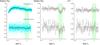 |
Fig. 1 Secondary eclipses of GJ 436b observed with the IRS (top) and MIPS (bottom) instruments. Relative flux offsets are applied to datasets for clarity. On the left, raw data are represented by cyan dots for the unbinned data and by black dots for binned data per interval of 7 min with their error bars. The superimposed red line is the best-fitting model and includes the transit model. On the middle, the same binned data divided by the best-fitting baseline model reveal the occultation shape. The eclipse model is superposed in red. The right panel displays the binned residuals from the same dataset. The shaded green area of every panel shows the eclipse event. |
2.2. IRS observations
On 2008 January 12, GJ 436 was monitored by IRS in the 16 μm peak-up imaging mode over a period of 6 h with an exposure time of 6.29 s. This program was sequenced without any dithering in three parts of which the middle consisted in the observation of GJ 436 while the two others targeted empty areas on the sky in order to obtain a high-S/N map of the background.
We discard the sky images because the photometric precision is not improved using them. We perform aperture photometry and partial deconvolution on the 1580 BCD images (version S17.2), and conclude as Knutson et al. (2009a) and S10 that the use of the PSF is to be preferred in the data reduction. Only deconvolution photometry is presented here.
The partial PSF constructed from the over-sampled PSF model given on the Spitzer website3 does not satisfactorily fit the data. We thus modify DECPHOT to simultaneously deconvolve a set of images. This technique attempts to find a unique partial PSF from the images themselves while it allows the position of the point source, its intensity, and the background to differ from an image to another. We use the same images both to determine the partial PSF and to perform deconvolution photometry. In a first step, we analyse twenty-five random images with our new version of DECPHOT to construct a satisfying partial PSF mode. In a second step, we deconvolve all images, one at a time and using as partial PSF model the result of the first step. The resulting normalised light curve is shown in Fig. 1.
2.3. IRAC transit and occultation photometry
In the context of the Spitzer programmes 541, 30129, 40685, 50051, 50056, 50734, 60003, and 70084, GJ 436 was monitored in the four channels of the IRAC camera at 3.6, 4.5, 5.8, and 8 μm. Those covered 16 occultations and 8 transits of GJ 436b, including a phase curve. In this work we perform for the first time a uniform analysis of these 29 IRAC time-series. Our analysis is based on the IRAC BCD images (version S18.18 for the two first channels and S18.25 for the last two). Because GJ 436 is a bright target for Spitzer with K ~ 6.1, it was observed in all 4 IRAC channels in subarray mode, meaning that every BCD is a set composed of 64 32 × 32-pixels subarray images. The telescope was not repointed during the course of the runs to minimise the motion of the star on the array. An exposure time of 0.08 s was used at 3.6 μm, 0.08 and 0.32 s at 4.5 μm, and 0.32 s for the two other channels. For more details on these IRAC observations we refer the reader to Table 1, Gillon et al. (2007a), Deming et al. (2007), Demory et al. (2007), Ballard et al. (2010a), S10, K11, and S12.
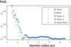 |
Fig. 2 Evolution of the photometric precision for raw data with the aperture radius according to different centring techniques in a complete dataset (e.g., AOR: 42614016). The 2D Gaussian adjustment (green asterisks) provides the best photometric precision for raw data in comparison to a centroid fit (magenta crosses), a double 1D Gaussian fit from the previously computed x- or y-FWHM (cyan boxes and red diamonds respectively), and a 1D Gaussian fit with a fixed FWHM (blue stars), in particular for small aperture radii. |
We reduce all the IRAC data with our EXOPHOT PyRAF4 pipeline to get raw light curves. We give a general overview of its routines below. For every subarray image, a 2D elliptical Gaussian profile fit is performed to determine the centre of the GJ 436 PSF. Aperture photometry is then accomplished with the IRAF/DAOPHOT5 software (Stetson 1987). Other centring approaches are tested (e.g., centroid fit and different double 1D Gaussian adjustments6) but with lower performance (Fig. 2). The background level is measured in an annulus extending from 12 to 15 pixels from the centre of aperture, and the resulting background flux in the aperture is subtracted from the measured flux for every image. For every channel, we compute the stellar fluxes in aperture radii ranging from 1.5 to 6 pixels by increments of 0.1. We select the aperture radius minimising the scatter of the residuals and their time correlation on the light curves corrected for instrumental and astrophysical effects (see Sect. 3). The chosen aperture sizes are all between 1.9 and 4.3 pixels (Table 1). Wider apertures lead to higher background contributions while smaller apertures lead to pixelation problems7 and significantly smaller counts (the IRAC PSF full-width at half maximum ranges from 1.2 to 2 pixels, depending on the channel).
For every block of 64 subarray images, we reject the discrepant values for the measurements of the x- and y-position, and the stellar and background flux using a 3σ median clipping. We generally discard up to 2 measurements from the 64 subarray images. Then the remaining measurements are averaged. We take the photometric error on the mean of the photometric error for every BCD set. At this stage, the first measurements of each light curve are discarded if they correspond to deviant values for all or some of the external parameters (detector or pointing stabilisation). In average ~10 min of data are rejected for each dataset (Fig. 3). Finally we perform a slipping median filtering for each light curve to discard outlier measurements due to, e.g., cosmic hits.
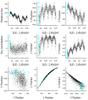 |
Fig. 3 For illustration, evolution of the parameters measured by our reduction pipeline for a randomly chosen IRAC dataset (at 3.6 μm, 2009 January 9, AOR: 28894208). From top to bottom and left to right we display the evolutions of the normalised stellar fluxes, the PSF x- and y-centres, the background values, and the PSF FWHMs in the x- and y-directions. The last three panels display the correlation diagrams for several parameters, revealing a clear dependence on the FWHM with the position for both directions. The first values (thick cyan coloured dots) are rejected, as the measured parameters (e.g., sky contribution) are not yet stabilised. |
We also test a photometric reduction of the IRAC data with DECPHOT, without improving results. Still we use DECPHOT to assess the infrared variability of GJ 436. Indeed, aperture photometry performed on deconvolved images reconvolved by the best-fitting partial PSF model allows us to derive the aperture corrections required for deriving the observed flux of the star F∗. For every dataset, we perform this procedure for a wide range of apertures. Then we average all the measurements and take the resulting value as the observed flux measurement for the dataset. The error on the mean is considered as its error bar. We apply the colour and inter-pixel corrections8. We do not correct the intra-pixel sensitivity as no complete correction map is available for the Warm Spitzer mission at the time of our analysis. The intra-pixel behaviour of the InSb detectors for the Warm Spitzer mission substantially differs from the one of the cryogenic phase9, making the correction map for the cryogenic phase unsuitable for all our data. The observed stellar flux F∗ is given in mJy for each IRAC dataset in Table 1. Their temporal evolution is shown in Fig. 4. The standard deviations of the fluxes are 0.77, 0.78, and 0.12% at 3.6, 4.5, and 8 μm, respectively. A fraction of the scatter in the shorter wavelengths should come from the absence of intra-pixel correction. GJ 436 thus appears to be a stable star in the IR. It is consistent with the nearly constant flux of the star in the optical over a period of five months as observed by K11 with the Automatic Photoelectric Telescope. Finally we convert the flux densities into Vega apparent magnitudes (presented in Sect. 3.4.2 with the magnitude of the planet) using Reach et al. (2005) magnitude calibrations on the stellar flux measured as it would be falling into a circular aperture radius of 10 pixels.
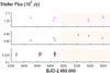 |
Fig. 4 Stellar flux evolution in the 3.6 (top), 4.5 (middle), and 8.0 μm (bottom) IRAC channels. The stellar flux slightly fluctuates with time in the 3.6 and 4.5 μm bandpasses, and is constant at 8.0 μm. A different inter-pixel map is used for the Warm mission data. The Warm Spitzer phase is shaded in pale pink for clarity. The flux modulation is probably due to the uncorrected intra-pixel effect and to the calibration uncertainties, which are not displayed here for clarity. |
We also test the noise pixel10 method of Lewis et al. (2013) to extract the fluxes of GJ 436. Based on the use of variable aperture radii, this method aims at minimising the correlation of the fluxes and the PSF centre positions. Our tests for the light curves in the 3.6 and 4.5 μm shows that this method leads up to 20% lower photometric precisions and larger time correlation of the residual light curves in comparison to traditional fixed aperture photometry and subsequent modelling of the position effects. It shows similar results only for a few datasets. Consequently, we do not use its resulting light curves in our analysis.
2.4. HARPS radial velocities
We used HARPS to record 171 spectra of GJ 436. Although GJ 436 was not part of the nominal volume-limited sample of M dwarfs (Bonfils et al. 2013) we used the same settings as for the other M stars to record its spectra. We observed without the simultaneous ThAr calibration and relied on the overnight ≲1 m/s stability of the instrument. This is a better mode for this V = 10.6 star because it leads to cleaner spectra and still with a photon-noise limited precision of 1 m/s with exposure times of 900 s.
Between 2006 January 25 and 2010 April 6, we obtained 171 measurements of which 44 were taken in a single night and the rest (127) was spread over the whole period. The measurements spread over the years generally have exposure times of 900 s, except some that were made with 1200 and 1800 s to compensate for non-optimal meteorological conditions. They have a median uncertainty of 1.0 m/s. The 44 observations taken on the same night (2007 May 10) aim at measuring the possible Rossiter-McLaughlin effect. They have exposure times of 300 s each and radial velocity uncertainties of 1.1−1.7 m/s. We note that one of the 127 measurements coincidentally falls during a transit event.
Extracted and wavelength calibrated spectra are delivered by the standard HARPS pipeline, as well as differential RVs obtained from the cross-correlation between the stellar spectra and a numerical template. To take full benefit of the many spectra of GJ 436 we merge them to derive a single high S/N template. We then use this template to re-compute the differential RVs by minimising the χ2 of the difference between this template and each spectrum. Using a merged stellar spectrum is a common alternative to a numerical template (e.g., Howarth et al. 1997; Zucker & Mazeh 2006). It was already used on HARPS by a part of our group (e.g., when we derived the RVs of GJ 1214, Charbonneau et al. 2009) as well as by other groups (e.g., Anglada-Escudé & Butler 2012; Anglada-Escudé & Tuomi 2012; Anglada-Escudé et al. 2013). Before modelling the data, we subtract its 0.34 m/s/yr secular acceleration (Kürster et al. 2003). Our implementation of the algorithm will be presented in a forthcoming paper (Astudillo et al. in prep.) and the inferred RVs are given in Table 2.
3. Data analysis
We choose to perform a global analysis of our extensive dataset to take full advantage of its observational constraints on the system parameters. Our Bayesian approach of the analysis is based on the use of the Markov chain Monte Carlo algorithm (MCMC, e.g., Ford 2006).
3.1. Data and model
In addition to the Spitzer photometry and the HARPS radial velocity measurements detailed in Sect. 2, we used the 59 Keck/ HIRES RVs presented in Maness et al. (2007) as input data in our global analysis to add further constraints on GJ 436b’s orbital and physical parameters. We also extend this analysis with a total of 29 transit times acquired with the Euler telescope (Gillon et al. 2007a), the Carlos Sanchez telescope (Alonso et al. 2008), the VLT (Cáceres et al. 2009), WISE and FWLO (Shporer et al. 2009), telescopes at the Apache Point Observatory (Coughlin et al. 2008), the HST (Pont et al. 2009; Bean et al. 2008), and the EPOXI mission (Ballard et al. 2010b).
An exhaustive description of the MCMC adaptive algorithm applied in this study can be found in Gillon et al. (2010, 2012). We use a model based on a star and a transiting planet on a Keplerian orbit about their centre of mass. For the RVs, a Keplerian 1-planet model is assumed. A model of the Rossiter-McLaughlin effect is also implemented following Giménez’ prescription (2006). We apply the model of Mandel & Agol (2002) to represent the eclipse photometry, assuming a quadratic limb-darkening law for GJ 436 and neglecting limb darkening for its planet. For each light curve, an analytical baseline model representing the flux variations of instrumental and stellar origin multiplies the eclipse model (see Sect. 3.3).
3.2. Input stellar parameters
Thanks to the interferometric measurement from von Braun et al. (2012), we have a strong constraint on the stellar radius value of 0.455 ± 0.018 R⊙. Deriving the mass of an M dwarf from a stellar evolution model is not as reliable as for higher mass stars (e.g., Torres 2013). To best benefit from this high-precision measurement and deduce a posterior distribution for the stellar mass independently from any stellar evolution model, we use the normal distribution N(0.455,0.0182) as prior distribution for the stellar radius. At each step of the MCMC, the stellar mass is directly computed from the stellar radius value (constrained by the interferometric prior) and from the stellar density value, which is constrained by the transit light curves (Seager & Mallén-Ornelas 2003).
For the atmospheric stellar parameters (effective temperature Teff, metallicity [Fe/H], projected rotational velocity Vsini, and surface gravity log g), normal prior distributions are assumed based on the following arguments: we take a value of 3416 K for the effective temperature (von Braun et al. 2012) derived from spectral energy distribution fitting and adopt a typical error value of 100 K for the case of low-mass stars (e.g., Casagrande et al. 2008); we use log g = 4.843 ± 0.018 from Torres (2007) as a first input before adopting those determined from the stellar mass and radius during the MCMC process; we derive a [Fe/H] of +0.02 inserting Schlaufman & Laughlin (2010)Δ(V − Ks) value into Neves et al. (2012) empiric photometry-metallicity relation, which is in good agreement with [Fe/H] = −0.03 from Bonfils et al. (2005) and [Fe/H] = +0.10 from Schlaufman & Laughlin (2010), and adopt the error of ±0.20 from Bonfils et al.; finally, we impose Vsini< 3 km s-1 (Delfosse et al. 1998) in the MCMC.
For the limb darkening, the two quadratic coefficients u1 and u2 are allowed to float in the MCMC. To minimise the correlations of these model parameters, those coefficients themselves are not used as jump parameters11, only their combinations c1 = 2 × u1 + u2 and c2 = u1 − 2 × u2 (Holman et al. 2006). For each transit, c1 and c2 are thus constrained by priors under the control of the normal prior probability distribution functions deduced from Claret & Bloemen’s tables (2011).
3.3. Baseline model
A baseline model aiming at representing systematic effects originating from several sources multiplies each transit/occultation model. It depends on the instrument and wavelength. In addition we include a thermal phase variation model to represent the 8 μm data. We describe the selection of our baseline model for every AOR in the next subsections.
3.3.1. The intra-pixel sensitivity and pixelation modelling
The main source of correlated noise in the IRAC InSb (3.6 and 4.5 μm) arrays is the dependence on the observed flux on the stellar centroid location on the pixel. These detectors show indeed an inhomogeneous intra-pixel sensitivity, which, combined with the jitter of the telescope and to the poor sampling of the PSF, leads to strong correlation of the measured fluxes with the position of the targets PSF on the array (e.g., Knutson et al. 2008, and references therein). It is known as the “pixel-phase” effect.
Our baseline models include two types of low-order polynomials to deal with the pixel-phase effect. The first one uses the prescription of Désert et al. (2009). It considers the dependence on the fluxes to the x- and y-positions of the PSF centre with the help of a polynomial that depends on the shift of the centroid centre on the array  (4)where dx and dy are the relative distance of the centroid from the pixel centre and a0 to a9 are free parameters in the fit.
The second one is motivated by the correlation of the FWHM with the PSF centroid location and with the stellar flux variation (Fig. 3). The following polynomial represents the dependence on the fluxes to the PSF FWHMs in the x- and/or y-directions  (5)where wx and wy respectively stand for the PSF FWHM in the x- and y-directions measured by our centring algorithm, and a10 to a16 are free parameters in the fit. Modelling this dependence is required for most IRAC InSb light curves.
Only the lowest frequencies of the pixel-phase effect can be modelled with the polynomial approach. For an improved modelling of the effect, Ballard et al. (2010a) and Stevenson et al. (2012a) demonstrated the efficiency of building a “pixel map” to characterise the intra-pixel variability on a fine grid. Here we combine the bi-linearly-interpolated sub-pixel sensitivity (BLISS) mapping method presented by Stevenson et al. (2012a) with the position/FWHM polynomial models. The BLISS mapping is performed at every step of the chain after the modelling of the polynomial models. This method maps the intra-pixel sensitivity at high resolution at every step of the MCMC from the data themselves. In our implementation of the method, a sub-pixel-scale grid of N2 knots along the x- and y-directions slices the sensibility map. We empirically set N in such a way that one average knot is never associated to less than 5 measurements to efficiently constrain the sensibility map. In most cases, we obtain a smaller scatter in the residuals using both parametric models and the sensitivity map.
3.3.2. The time varying sensitivity modelling of the detectors
Another well-documented detector effect, especially important for the Arsenic-doped Silicon (Si:As) material instruments (IRAC 5.8 and 8 μm, IRS 16 μm), but also present in the InSb ones, is the increase of the detector response at the start of AORs. The so-called “ramp” is attributed to a charge-trapping mechanism resulting in a dependence on the gain of the pixels to their illumination history (e.g., Knutson et al. 2008). Following Charbonneau et al. (2008), we model this ramp with a polynomial of the logarithm of time.
Besides, we also test linear and quadratic functions of time in our baseline models to check time-dependent trends of instrumental and/or stellar origin.
3.3.3. Phase curve modelling
As thermal emission is isotropic, the emission of an atmospheric layer is analogous to the scattering of incident light by a Lambert surface (Seager 2010). Assuming that one specific atmospheric layer dominates the emission at a given wavelength, the thermal phase curve of a pseudo-synchronised planet on an eccentric orbit can be modelled by the following function 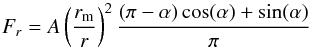 (6)where A is the thermal day-night contrast for a circular orbit, r is the distance between the star and the planet, and rm is its average. The last fraction models the phase variation of a Lambert sphere (Russell 1916), with α being the phase angle. It can be easily found with the relation cos(α) = sin(ω + f)sin(i) (e.g., Sudarsky et al. 2005), where i is the orbital inclination, ω is the argument at periapsis, and f is the true anomaly. This baseline model alone supposes a constant stellar flux during the observation time but takes the received stellar radiation variation with time into account according to the planet-star distance (e.g., Kane & Gelino 2010; Cowan & Agol 2011). The phase curve modelling implies the insertion of A and the phase offset in the phase angle as jump parameters.
3.4. Fitting procedure
A preliminary evaluation of all the necessary input parameters in our MCMC code is done before performing a global analysis of the GJ 436 dataset. Furthermore, the multiple observations within the same filters allow us to search for variability in the eclipse parameters.
3.4.1. Model selection and error rescaling
For each light curve (corresponding to a specific AOR), we test a wide range of baseline models and look for the minimisation of the Bayesian Information Criterion (BIC, e.g., Gideon 1978) to select the simplest model that best fits the data (Occam’s razor). We aim at detecting the thermal phase curve at 8 μm prior to the global analysis. However its amplitude is not significant at a 3σ level and the baseline model for the phase curve modelling (Eq. (6)) does not minimise the BIC, making it useless in the global analysis. Afterwards we test it again with prior constraints from the global analysis without better success (Sect. 5). The MIPS light curves corresponding to the 14 different dithered positions are treated separately to take the spatial inhomogeneity of the detector response into account. Apart from a rescaling normalisation no baseline model is applied to the individual MIPS light curves.
Once we have selected the baseline models for all AORs, we perform a preliminary MCMC analysis (two chains of 80 000 steps) to assess the need for rescaling the photometric errors. For each AOR, the ratio of the residuals’ standard deviation and mean photometric error is stored as βw. This factor approximates the required rescaling of the white noise of each measurement. To take the correlation of the noise into account, a scaling factor βr is determined through the “time-averaging” method (Pont et al. 2006) in which the scatter of individual points and the scatter of binned data with different time intervals are compared with the expected scatter of the corresponding binned data without the presence of correlated noise. The highest values of βr are kept. At the end, the error bars are multiplied by the corresponding correction factor CF = βw × βr. The values of βw and βr derived for each AOR are given in Table 1. The βw values are generally higher than unity, indicating the undervaluation of photometric errors, e.g. the photometric IRAC errors on the mean are lower than the real photometric errors. Besides, light curves with βr> 1 highlight our inability of our models to perfectly represent the data (due to instrumental and/or astrophysical effects). For the RVs, both our minimal baseline models correspond to a scalar representing the systemic velocity of the star. To compensate both instrumental and astrophysical effects that are not included in the initial error calculation, the “jitter” noises of 3.8 (Keck/HIRES) and 1.7 m s-1 (HARPS) are quadratically added to the error bars to equal the mean error to the standard deviation of the best-fit residuals.
3.4.2. Global analysis
Once the models selected and the errors rescaled, we perform a global MCMC analysis of our dataset to probe the posterior probability distributions of the jump and physical parameters. Two chains of 240 000 steps compose this analysis. We successfully check their good convergence and mixing with the statistical test of Gelman & Rubin (1992), all jump parameters showing indeed a value close to 1 at the 0.01 level. The resulting median values and 68.3% probability interval for the jump and physical parameters are given in Table 3. The fitted light curves are compared with the data in Figs. 1, 5–7. Note that the light curves are not binned prior to the analysis (except for the subarray images, see Sect. 2.3). The fitted radial velocities are displayed in Fig. 8. Unfortunately, the Rossiter-McLaughlin effect is not detected. We also try to model the Rossiter-McLaughlin effect with the implementation of Boué et al. (2013) but results are not conclusive either. According to Winn (2010), we can expect to observe a maximum amplitude of the RV anomaly ΔVRM ~ 4 × 10⁻³ × Vsini ~ 12 m s-1 considering a maximum projected rotational velocity of 3 km s-1. However one should better expect ΔVRM ~ 1.92 m s-1 assuming a stellar rotation of 48 days (see Sect. 4.3).
System parameters derived from our global analysis of the Spitzer data and radial velocities.
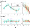 |
Fig. 8 Top: radial velocities measured with the HIRES and HARPS spectrographs. The data are period-folded on the best-fit transit ephemeris, the 0 of the x-axis corresponding to the inferior conjunction time. The fit is superimposed on red and the respective residuals are shown on the bottom panel. The left panels display those corresponding data during the whole planetary orbit and the right ones are a zoom on the box to highlight the (undetected) Rossiter-McLaughlin effect. The HARPS binned data are added in black diamonds filled white for clarity. |
From the inferred planet-star flux ratios we retrieve the brightness temperature Tbright of the planet assuming the planet emits as a blackbody in the different Spitzer bandpasses and using a Phoenix stellar atmosphere model (Hauschildt et al. 1999) (with Teff = 3400 K, log g = 5.0, and solar metallicity, Table 4). We warn the reader that the error bars do not take the error of the model into account. We finally derive the magnitude of the planet in the different IRAC bandpasses.
Planetary brightness temperatures evaluated for every instrument/bandpass.
Apparent and absolute magnitudes of GJ 436 and its planet.
3.4.3. Analysis allowing for transit and occultation variations
Our global analysis assumes a constant transit depth and duration, orbital period, and occultation depth at every wavelength. Even if the resulting model fits very well our data, some variations may indicate diverse physical phenomena which are relevant enough to be verified. For this purpose, we conduct new MCMC analyses, benefiting from the strong constraints brought by the global analyses to attain the highest sensitivity.
First we check if the transit depth dF varies with wavelength. It provides the apparent radius of the planet, which gives in return a piece of the transmission spectrum of the terminator of the planet. We thus perform three separate additional MCMC analyses for each of the three relevant IRAC channels (3.6, 4.5, and 8 μm) considering only the light curves including a transit. We use a uniform prior distribution for dF and assume normal prior distributions for the other jump parameters based on the posterior distributions resulting from our main global analysis (Table 3). We cannot detect any significant chromaticity of the transit depth (Table 6, Fig. 9, and Sect. 5).
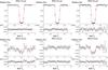 |
Fig. 9 Detrended Spitzer 3.6 μm (left), 4.5 μm (middle), and 8 μm (right) photometry folded on the best-fit transit ephemeris obtained in our analysis per channel for the transits (top, Sect. 3.4.3) and in our global analysis for the occultations (bottom). The best-fit eclipse models are superimposed. |
Transit depth variation with wavelength.
Individual measurements of the occultation depths for the different AORs (Sect. 3.4.3).
Then we test the transit and occultation depth variations as a function of time within a given instrument. Such transit depth variations could reveal a physical change of the radius with time (for e.g. due to the thermal expansion of the atmosphere or the presence of variable clouds) or stellar activity (see K11 for all those aspects). Besides, the occultation depth fluctuation should provide constraints on general circulation models. We separate all light curves including an eclipse event in groups according to their channel origin and perform new MCMC analyses for each group separately. We set the transit and occultation depths as jump parameters for each individual eclipse and keep the other parameters as normal prior distributions based again on our global analysis (Table 3). We find no significant occultation depth variation (Table 7 and Fig. 10 for the data at 8 μm), and no transit depth variation contrary to B11 and K11 studies (Fig. 11 and Table 8).
The transit duration variation, which might be due to the presence of another orbiting body such as a moon (e.g., Kipping 2009), is the third parameter we examine. Because it might be linked to a transit depth variation, we set those two parameters as jump parameters in our MCMC analyses and maintain normal prior distributions for the other parameters. We perform individual MCMC analyses on each time-series recording a transit. We do not detect any significant transit duration variation (Fig. 11 and Table 8).
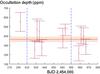 |
Fig. 10 Occultation depth variation at 8 μm as function of time. Brown diamonds with their 1σ-error bar represents occultation depths. The dashed blue lines indicate temporal caesura in the x-axis. The red horizontal line displays the eclipse depth value obtained during the global analysis and the shaded region surrounding it is its 1σ-error bar. |
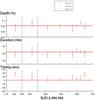 |
Fig. 11 Transit parameter variations. From top to bottom, the plots respectively show the transit depth, the transit duration, and the transit timing variation with their error bars according to time for the different IRAC channels. The pink dots stand for the 3.6 μm channel, the green crosses for the 4.5 μm channel, and the brown diamonds for the 8 μm channel. The vertical dashed blue lines indicate temporal caesura in the x-axis. The horizontal red lines present in the two top panels respectively indicate the transit depth and duration derived from the global analysis. The shaded surrounding area is its 1σ error bar. |
Finally, we search for transit timing variations (TTV), which may disclose the presence of another orbiting body in the system (Holman & Murray 2005; Agol et al. 2005, and references therein). We perform a new individual analysis of the transit light curves, keeping all the parameters except the mid-transit times under the control of Bayesian penalties based on the results of our global analysis. The measured timings are given in Table 8. When compared with the transit ephemeris deduced in our global analysis, they do not reveal any significant TTV (Fig. 11, bottom panel).
3.4.4. Flares-like structures in the light curves
Previous studies of GJ 436 Spitzer datasets reported structures that could potentially be attributed to stellar flares. The first one was signalled just after an occultation at 3.6 μm (2008 January 30, AOR: 24882688) by S10 and B11, and led to contradictory results. Their opinions diverged on how to take care of the post occultation spike they both identified. On our side, we notice that the amplitude of the structure highly depends on the chosen aperture radius, and disappears for aperture radii below 2.1 pixels (Fig. 12). The insertion of Eq. (5) in the baseline model leads to a significantly decreased occultation depth (~170 ppm instead of ~535 ppm) and to a higher photometric accuracy (mean photometric error ~5.11 × 10⁻⁴ instead of 10.30 × 10⁻⁴, Fig. 12), which we assign to the strong evolution of the FWHMs during the occultation. Thanks to the inclusion in our modelling of the impact of the FWHM variations, a series of tests reveal that our measured occultation depth of 169 ± 48 ppm is not dependent on the selected aperture radius or on the rejection of a fraction of the post-occultation data, demonstrating its robustness.
Individual transit parameters.
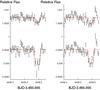 |
Fig. 12 Influence of the chosen aperture radius and the baseline modelling. We present the same light curve (at 3.6 μm, 2008 January 30, AOR: 24882688) four times, however showing different noise level and a different occultation depth due to the data reduction and analysis. On the left, the aperture photometry is centred by a 2D elliptical Gaussian fit with an aperture radius of 1.9 pixels, while on the right the aperture radius equals 3.5 pixels. They all proceed to the same MCMC analysis with the inferred parameters from Table 3, except that the top ones contain a baseline model dealing with the measured PSF FWHM, while the bottom ones do not. |
The second occultation time-series at 3.6 μm was supposed to confirm or infirm S10 and B11 interpretations but another flare-like structure was recorded during the occultation by S12 (see Fig. 6, second light curve from the top, 2011 February 1, AOR: 40848384). In this case, we cannot identify any sharp variation of an external parameter able to explain it. We try to measure the occultation depth when discarding (or setting a zero-weight on) the last flux measurements that show a net discrepancy but the occultation depth cannot be constrained. So we cannot discuss the influence of this flare-like structure on the occultation depth measurement. The addition of this light curve to our global analysis cannot give a strong confirmation (217 ± 140 ppm) of our first 3.6 μm occultation depth measurement but agrees with it.
We finally report another flare-like structure during an observation of GJ 436 at 3.6 μm. This one happened outside a scheduled eclipse (2010 June 23, AOR: 38807296, Fig. 13). We cannot remove this peak with any of our baseline models. However, for that AOR we notice a surprising absence of correlation between the noise pixel parameter and the measured PSF FWHM (Fig. 14), suggesting again an instrumental origin of the photometric structure. In the end, we can only identify one flare-like structure of which the origin is probably instrumental (cosmic hit in the PSF core), considering the absence of other similar structures in our extensive dataset and the extreme quietness of GJ 436. Indeed, the SHK index, a proxy for stellar activity, measured from the HARPS spectra is weak in comparison to the Ca ii H&K emission of similar type stars and does not significantly vary on short time scales (Astudillo et al., in prep.).
4. Planetary companion
In this section, we present the search for a second planet orbiting GJ 436, which we perform on the residual light curves and the HARPS RVs. We also discuss the two potential transiting companions found recently by S12 in some Spitzer datasets.
4.1. Search in the residual light curves
We analyse the best-fit residual light curves resulting from our global MCMC analysis in order to be detached from GJ 436b eclipses and from any instrumental systematics. We use our own version of the algorithm MISS MarPLE (Berta et al. 2012) on the residual light curves.
We can identify only two potential transit-like events. The strongest one corresponds to a transit depth of ~150 ppm lasting for 0.5 h at BJD = 2 455 376.702 with a ~4σ significance. The second one recovers a signal of only a 3.1σ significance at BJD = 2 455 585.686 and lasts for 0.6 h with a depth of ~100 ppm. It should be noted that the correlated noise is not fully taken into account when estimating those significance levels. The actual significance of both structures is clearly marginal, as can be judged by eye in Fig. 15. With 1475 measurements from both light curves and 4 more degrees of freedom for the transit model, a Δχ2 = −6 between the transiting and non-transiting companion model corresponds to a ΔBIC = −6 + 4 log(1475) = +6.7. Using the BIC as a proxy for the model marginal likelihood (Kass & Raftery 1995), this ΔBIC results in an approximated Bayes factor of eΔBIC/2 ~ 28 in favour of the non-transiting companion model.
These two transit-like features (Fig. 15) were also detected by S12 although with a higher depth and longer duration. These authors attributed them to their planet candidate UCF-1.01.
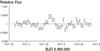 |
Fig. 13 Flux modulations present in the 2010 June 6 Spitzer light curve (AOR: 38807296) during GJ 436 monitoring. |
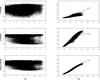 |
Fig. 14 Lack of correlation on the PSF FWHM of GJ 436 (AOR: 38807296) with the square root of the pixel noise parameter ( |

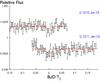 |
Fig. 15 Transit-like structures detected in two residual light curves by our own version of the code MISS MarPLE (Berta et al. 2012). For both structures, a box-like model illustrates a transit depth of 120 ppm and a duration of 0.6 h. |
Assuming that both structures correspond to two transits of the same and still undetected planet, the elapsed time between the two signals gives a maximum period of ~208.98 days while the transit duration regarding a central transit returns a minimal period of 0.098 day. The lack of a continuous monitoring between these two potential transits prevents us from identifying a single period. Still, our extensive dataset allows us to discard many fractions of 208.98 days for which at least a third transit should have been present in the Spitzer data. Injecting fake transits at the corresponding phases, we check our ability to recover them in the Spitzer data with MISS MarPLE for each period and each expected transit. Fig. 16 shows the period ranges that we can keep from these tests. In this figure, the periods too close to GJ 436b’s one are also discarded to allow the dynamical stability of the system (from ~1.8 to ~3.9 days, Ballard et al. 2010b). In the end 40 possible periods remain. One may assess their replicability with new ultra-precise time-series photometry based on the ephemeris 2 455 476.702 + N × 208.98 days. For the sake of completeness, we also analyse the residual light curves with two versions of the algorithm BLS (Kovács et al. 2002) (the optimal BLS from Ofir 2014 and the BLS available on the NASA Exoplanet Archive website12), which searches for periodic box-shaped structures in photometric time-series. We fail to detect any significant signal.
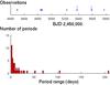 |
Fig. 16 Top: timing of GJ 436 observations with the 3.6 and 4.5 μm IRAC channels. The two vertical lines indicate the datasets having the transit-like features. Bottom: distribution of the possible period range for the putative additive transiting planet. The observational coverage discards all periods below 1.18 days. |
4.2. Discussion on a putative GJ 436c
S12 proposed two planetary candidates in the GJ 436’s stellar system and named them temporarily UCF-1.01 and UCF-1.02 until their confirmation. They observed UCF-1.01 transits during 2008 July 14, 2010 January 28, 2010 June 29, 2011 January 24, and July 30 datasets. UCF-1.02 potential transits occurred during both of those 2010 datasets.
In our analysis we pay particular attention to the behaviour of the measured external parameters. The following two examples may cast doubt on some observations of S12’s candidate transits. A change of the background contribution (Fig. 17) indeed affects the 2010 January 28 dataset just at the end of the observation of UCF-1.01 transit, while a higher x-FWHM alters the 2008 July 14 light curve during another UCF-1.01 transit. Ballard et al. (2010a) also discarded the latter example because only small photometric apertures reveal a transit-like shape.
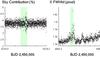 |
Fig. 17 Atypical behaviour of measured parameters during two of S12’s UCF-1.01 transits. Left panel: background contribution discontinuity around BJD 2 455 225.09. Right panel: points out a strong fluctuation of the x-FWHM around BJD 2 454 662.32. UCF-1.01 transit events are shaded in green. |
The S/N quality of our residual light curves being sufficient to identify transit shapes similar to S12, we must also verify that our adopted baseline models are not responsible for the subtraction of the transit signals. We thus insert the transit signals observed by S12 in our original light curves and perform individual MCMC to get new residual light curves. We look for transit-box shapes on the individual residual light curves with the previous manner and identify the injected transits with more than 4σ confidence. Our models correcting for instrumental systematics do not destroy transit signals.
We wonder why our results diverge. We both opted for a similar aperture radius (S12: 2.25 px; our study: 2.2 px) and for a BLISS mapping in the 2010 January 28 dataset, but we differ in the choice of the centring technique. S12 employed their time-series image de-noising for this purpose before centring with a Gaussian whereas we use a 2D elliptical Gaussian fit. We can obtain a similar structure to S12 (Fig. 18), if we centre the PSF with a double 1D Gaussian having the computed x-FWHM and do not model the light curve with the FWHMs (Eq. (5)), but the UCF-1.01 transit S/N remains very low. Likewise, a similar transit-like shape in the 2011 July 30 light curve is found using the same aperture radius as S12 (5 px) with a PSF centring obtained by a double 1D Gaussian fit (Fig. 19) and with the same baseline as the one from our analysis. However, the transit is not significant (~1σ).
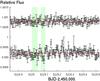 |
Fig. 18 Highlight on the impact of the data reduction/analysis details on the presence of low-amplitude transit-shaped structures in the Spitzer photometry (2010 Jan. 28, AOR: 38702848). We apply relative flux offsets in the above two plots for clarity. The upper dataset is the result of aperture photometry with a 2D elliptical Gaussian centring while the lower one is done with a double 1D Gaussian fit. The upper is corrected with a baseline involving the measured FWHM while the lower is not. Black dots are the binned data per interval of 5 min with 1σ error bars. The supposed UCF-1.01 (right) and UCF-1.02 (left) transit events are shaded in green. |
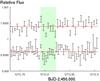 |
Fig. 19 Same as Fig. 18 for the 2011 Jul 30 data (AOR: 42614016). The upper dataset is the result of aperture photometry with a 2D elliptical Gaussian centring and is corrected for all systematics minimising the BIC. The lower dataset is produced from a double 1D Gaussian fit of the computed x-FWHM and corrected in the same way. The shaded green area corresponds to UCF-1.01 transit event. |
4.3. Analysis from the radial velocity residuals
The standard deviation for the RV residuals around a Keplerian solution composed of a single planet is 1.53 m/s, its mean error of 0.02 m/s, and the resulting χ2 of 2.0 ± 0.2. In their periodogram corresponding to the one planet + drift model (Fig. 20), we identify several peaks although none shows a significant power excess. Eight peaks have power excess above the 1σ-significance level (which corresponds to a power p = 0.131). They have periods 1.0181, 1.0417, 1.266, 2.000, 4.70, 23.4, 48.8, and 263 days with powers 0.142, 0.146, 0.131, 0.155, 0.138, 0.136, and 0.142, respectively. We note that one is at about twice the period of GJ 436b, at 4.7 days. We also identify a peak around 48 days, which is reminiscent of the rotational period identified by Demory et al. (2007) (which differs from the rotational period identified by photometry by K11, P ~ 57 days) based on spectral indices for a sub-sample of our HARPS spectra, and another power excess around 23 days, i.e. about half the 48-day period and thus possibly a harmonic. Nevertheless, they all have a power much below the power threshold for the 3σ-confidence level ( ) and we therefore cannot draw any firm conclusion. Assuming that the residuals are only noise, Fig. 21 shows the detection limit, which, for a given period, delineates the mass limit above which a planet on a circular orbit is excluded (with a confidence level of 99% and for 12 randomly chosen trial phases, see Bonfils et al. 2013). We see that for specific periods, we can exclude planets with masses higher than Earth-mass and reject planets with masses above 10 Earth masses for periods up to few-hundred days. We exclude super-Earths more massive than 3–5 Earth masses in GJ 436’s habitable zone, which is spread from 0.121 and 0.330 AU basing on Selsis et al. (2007) criteria. The analysis of the RV residuals cannot constrain the presence of UCF1.01 and UCF1.02 given that their small radii (~0.7 R⊕) should correspond to masses lower than our upper-limit mass.
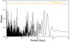 |
Fig. 20 GJ 436 periodogram of the residuals for the model composed of 1 planet on a Keplerian orbit plus 1 drift. The horizontal yellow line represents the 1% false alarm probability. No peak shows a significant power excess. |
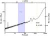 |
Fig. 21 Conservative detection limits on Mpsini applied to GJ 436 residual RV time-series around a chosen model (composed of planets, linear drifts, and/or a simple sine function). Planets above the limit are excluded, with a 99% confidence level, for all 12 trial phases. The vertical dashed yellow line marks the duration of the survey. |
5. Atmospheric analysis
In order to use our new measurements to draw inferences on the atmospheric properties of GJ 436b we employ a number of atmospheric modelling tools. We first derive planetary pressure-temperature P–T profiles using the 1D plane-parallel model atmosphere code described in Fortney et al. (2005, 2008). The opacity database is described in Freedman et al. (2008) and the equilibrium chemistry calculations in Lodders & Fegley (2002). We use the base solar abundances of Lodders (2003).
We first generate thermal emission spectra for models representative of conditions on the dayside of the planet. Within the framework of the thermal emission calculations, we are constrained to pre-tabulated equilibrium chemistry abundances. In Fig. 22 we plot two models. One uses solar abundances and the other 50×-solar, broadly similar to the carbon abundance in Uranus and Neptune (Baines et al. 1995). At higher metallicity, hydrogen-poor molecules such as CO and CO2 become more abundant (Lodders & Fegley 2002), with the mixing ratio of CO rising linearly, and CO2 quadratically, with metallicity. While this metal-enhanced model certainly goes in the right direction towards reproducing the large measured flux ratio differences between the 3.6 and 4.5 μm IRAC bandpasses, the fit is not satisfactory and our occultation depth at 3.6 μm, which is smaller than S10’s, is still too high to be explained by a CH4 fluorescence with only stellar photons (Waldmann et al. 2012). S10 and Madhusudhan & Seager (2011) have previously shown that extraordinarily low CH4 mixing ratios, along with high CO and/or CO2 abundances are needed to reproduce the previous S10 observations. We concur on this point based on our measurements. Inversion techniques could be used on to better constrain the atmospheric abundances (e.g., Madhusudhan & Seager 2011; Line et al. 2012).
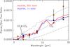 |
Fig. 22 Model planet-to-star flux ratios compared to the observed Spitzer occultation data. Both models assume a hot day side, with absorbed energy redistributed only over the dayside. The blue model uses solar metallicity, while the red model uses 50×-solar. The Spitzer data are orange circle while the model band averages in the six bands are shown as coloured squares. The location of prominent absorption features that differ between the models (where CO and CO2 absorb strongly) are labelled. The planet-to-star flux ratios of 500, 700, and 900 K blackbodies are shown in dashed black. |
In Fig. 23 we compare our Spitzer depths to two models from Moses et al. (2013) that were created to better fit the previous Spitzer depths derived by S10. The model labelled “best-fit retrieval” used the Bayesian inversion methods of Line et al. (2013, 2014) to find a best-fit spectrum, with free parameters that include the P − T profile and chemical mixing ratios. The “300×-solar” model uses a Line et al.P − T profile, but mixing ratios from a detailed non-equilibrium chemistry calculation for an atmosphere enriched in metals by a factor of 300 over solar abundances. It is clear that reduced secondary eclipse depths at 3.6, 5.8, and 8.0 μm from our analysis lead to a poor fit from these models. Given these lower fluxes, it appears plausible that a cooler atmospheric P − T profile would better fit these data, and also yield a lower flux in the 4.5 μm band, which has always been problematic to fit (S10; Madhusudhan & Seager 2011; Moses et al. 2013). It does appear that some CH4 depletion and CO/CO2 enhancement will still be needed to match 3.6 and 4.5 μm band depths, given our models presented in the previous plot (Fig. 22). Also, cooler day-side temperatures may allow for a fit with a lower metallicity, and hence less CO2, and a better fit at 16 μm, which includes a strong CO2 band.
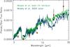 |
Fig. 23 Comparison of our observed Spitzer occultation data with synthetic emission spectra for GJ 436b from Moses et al. (2013). The green and blue curves correspond respectively to the best fit retrieved model, given S10 data, using the method of Line et al. and the 300×-solar model. The model band averages in the six bands are shown as coloured squares. Our Spitzer data are shown as orange circles. |
We next turn to the transmission spectrum of the planet to examine whether a large abundance of CO and CO2, and corresponding small mixing ratio of CH4, are also consistent with this dataset. For this purpose, we complete our Spitzer transit depths with those from EPOXI (Ballard et al. 2010b, 0.35–1.0 μm), HST WFC3 (Knutson et al. 2014, 1.14–1.65 μm), HST NICMOS (Pont et al. 2009, 1.1–1.9 μm), and from the ground in the H and K bands (Alonso et al. 2008; Cáceres et al. 2009) in Fig. 24. Here we model the planetary transit radius, which is inferred from the transit depth and von Braun et al. (2012) stellar radius (0.455 R⊙), as a function of wavelength, using the transmission spectrum code described in Fortney et al. (2003, 2010). The transmission spectrum of the planet GJ 436b was previously modelled in some detail with this code by Shabram et al. (2011). An advantage of these calculations is that we are able to model arbitrary chemical mixing ratios, rather than equilibrium chemistry.
We first compute the transmission spectrum of the 50×-solar model, shown in Fig. 24 in orange. We compare to the two best-fit chemical models of S10 in red and blue, which use low CH4, and high CO and CO2 mixing ratios. The models differ dramatically in the optical only because it is unclear if the neutral atomic alkalis Na and K are still present in the planetary atmosphere, or have condensed into clouds. The equilibrium chemistry model is strongly disfavoured by the Spitzer data, as it yields the wrong planetary radius ratio between the 3.6 and 4.5 μm bands. The blue and red curves reproduce the Spitzer data better. This is consistent with the dayside occultation data, where models with strongly enhanced CO and CO2, and strongly depleted CH4 are preferred.
We also note that deviations from a constant radius model are not particularly significant. This could suggest that cloud material obscures the transmission spectrum (e.g., Fortney 2005). Alternatively, the atmospheric mean molecular weight could be higher that assumed. A very metal-rich atmosphere would shrink the scale height as well as produce abundant “metal-metal” species such as CO and CO2, which is certainly needed to explain the dayside spectrum.
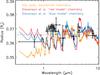 |
Fig. 24 Model transit radius as function of wavelength compared with published transit depths and our Spitzer results. From left to right, the radii are derived from EPOXI (Ballard et al. 2010b), HST WFC3 (represented by empty diamonds with thinner error bars in the 1.14–1.65 μm wavelength range, Knutson et al. 2014), HST NICMOS (Pont et al. 2009), the H and K bands from the ground (Alonso et al. 2008; Cáceres et al. 2009), and IRAC (ours) studies. Three models are shown. In orange is the 50×-solar model from Fig. 22. In red and blue are transmission spectra taken from Shabram et al. (2011), who used mixing ratios suggested for the planetary dayside by S10. Band-average calculations are shown as squares for the three models, across the Spitzer bandpasses. The dramatic differences between the models at optical wavelength are only due to different assumptions about the abundances of alkali metals. The blue and red models, which have depleted CH4, and enhanced CO and CO2, are generally preferred. |
Our phase curve fit (Fig. 25) presents a phase offset of  , a day-night contrast parameter
  ppm, which is not significant at a 3σ level, and a peak-to-peak flux difference of 268 ppm. Those latter two values should be identical for a circular orbit model being perpendicular to the sky plane. We compare our phase curve fit with the 3D coupled radiative transfer and general circulation model adapted to GJ 436b by Lewis et al. (2010) (Fig. 25). It takes the pseudo-synchronous rotation of GJ 436b and the atmosphere metallicity into account. The 1×-solar atmospheric metallicity case of GJ 436b (represented by green stars) does not fit the observations while the 50×-solar case (magenta circles) gets closer to them. If revealed significant, the amplitude disparity between the 3 light curves would require a (very) metal-rich atmosphere (>50×-solar) to explain the high day/night temperature contrasts. Indeed, at higher metallicity, photons are absorbed and emitted from lower pressures, where the radiative timescale is short, making temperature homogenisation more difficult. This result would be in good qualitative agreement with our transmission and emission spectra analysis.
6. Discussion
6.1. On the host star
We could not find any hint of stellar activity (large amplitude trend, convincing flare-like structure) in our photometric time-series for GJ 436. A low stellar activity for GJ 436 is supported by the stable stellar flux (Fig. 4), and by the temporal stability of the transit depths. In our light curves, we detect no occultation of stellar spots by the planet during its transits. Neither do Knutson et al. (2014) in their HST WFC3 data. This is in good agreement with the advanced age of the star deduced from its kinematics (Leggett 1992) and weak chromospheric Ca ii H and K emission lines (Butler et al. 2004).
Our global analysis gives a stellar mass of  . This value is higher than what Delfosse et al. (2000) obtain from mass-luminosity relations partly calibrated with eclipsing binaries (0.44 ± 0.04 M⊙). Our error on the stellar mass strongly depends on the stellar radius error. Multiplying by a factor two the stellar radius error almost doubles our uncertainty on the stellar mass (ΔM∗ = 0.141 M⊙). The fact that GJ 436 appears as a M2.5 star despite its somewhat high mass might reflect an effect of the metallicity. Indeed, the stellar spectral type depends both on the mass and metallicity : for a given mass, the more metal-rich a star is, the lower its effective temperature is. For instance, GJ 436 mass and temperature agree with Spada et al. (2013) models for a solar or supersolar metallicity (Fig. 26) as supported by our derived metallicity, and by e.g. Johnson & Apps (2009) and Neves et al. (2013) with [Fe/H] = +0.25 and +0.02 respectively.
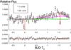 |
Fig. 25 Top: the observed phase curve of GJ 436 at 8 μm (2008 July 12, AORs: 27863296, 27863552, 27863808) superimposed to a model for a Lambert sphere (red line). The adopted baseline models are respectively p([xy] |


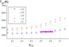 |
Fig. 26 Theoretical effective temperature-mass relations from the stellar evolution model of Spada et al. (2013), with the mixing length parameter α set to 0.5. Theoretical 4 Gyr isochrones are plotted for different metallicities indicated by legend. The magenta filled box shows the GJ 436 position on the diagram according to von Braun et al. (2012)’s stellar temperature and our inferred stellar mass. |
6.2. On the atmospheric model
Our findings fit in reasonably well with recent theoretical advances. Motivated by previous observational work on GJ 436b, there have been recent suggestions along multiple theoretical lines that Neptune-class exoplanet atmospheres may commonly have extremely high metallicities, perhaps several hundred times solar, or higher. Fortney et al. (2013) have suggested, based on atmospheric accretion of planetesimals in population synthesis formation models, that high atmospheric metallicities may be a common outcome of the planet formation process. Moses et al. (2013), in a detailed chemical study of GJ 436b, suggest that low CH4 abundances, and high CO and CO2 abundance can be a natural outcome in an atmosphere where metals are so abundant that H2 is no longer the dominant atmospheric constituent, by number. Independently, Agúndez et al. (2014) favour models with an efficient tidal heating and also a high metallicity. Finally, the featureless transmission spectrum extracted by Knutson et al. (2014) leads to an atmospheric metallicity of 1900 times solar or to a cloud layer at pressure below 10 mbar. It is not clear if such high envelope metallicity is consistent with the radius and bulk density of the planet. We suggest continuing chemical studies of the atmosphere of GJ 436b with our revised occultation and transit depths. It may possibly favour a high cloud seen in transmission without such a high atmospheric metallicity. Future comparisons with GJ 3470b (Bonfils et al. 2012; Crossfield et al. 2013; Venot et al. 2014; Demory et al. 2013) will also be illuminating.
7. Conclusion
We performed an independent and global analysis of all available Spitzer data for GJ 436 combined with our new HARPS RV measurements. In this analysis, we optimised the data reduction procedure for each Spitzer instrument with the adaptation of partial deconvolution photometry or aperture photometry, and we paid a particular attention to the modelling of the systematic effects. We recommend the use of the FWHM of the PSF in both directions as parameters to model the instrumental systematics. The insertion of the HARPS RVs complements well the photometric data. Our results are globally consistent with previous studies (e.g., S10; B11; K11; S12) but some discrepancies disclose another facet of GJ 436b. In particular we obtained constant values of the transit depth with time, a flat transmission spectrum, and a significantly lower 3.6 μm emission.
GJ 436b is a warm Neptune with a mass of 25.4 ± 2.0 M⊕ and a radius of 4.096 ± 0.162 R⊕. It is in an eccentric orbit (e = 0.162 ± 0.004) around a M2.5 star (0.56 ± 0.06 M⊙). We detect no stellar variability (no stellar flux variation on a large scale and no transit depth variation with time) in the whole set of Spitzer light curves. No occulted star spots were observed in the transit light curves. K11 observed very weak photometric activity in the optical. In addition, Astudillo et al. (in prep) measure a SHK index in the HARPS spectra that is consistent with a weak stellar activity and does not show a detectable periodicity. We thus confirm GJ 436’s weak activity.
Neither the amplitude of the phase curve nor its shape can be constrained with the current dataset. We recommend new observations with future facilities at multiple wavelengths longer than 8 μm combined with stellar monitoring at shorter wavelengths, such as 4.5 μm or in the visible to discern the planetary phase curve from stellar variability. Such observations should constrain longitudinal properties of the atmosphere at different depths.
Despite our shallower occultation depths at 3.6, 4.5, and 8 μm compared to previous works, all the photometric Spitzer time-series are still in good agreement with a metal-rich atmosphere depleted in methane and enhanced in CO/CO2. However the metallicity of the atmosphere may not be as high than previously thought. A cooler atmospheric model with disequilibrium chemical abundance profiles should better fit our data, and also yield a lower flux in the 4.5 μm band, which has always been problematic to fit. We encourage an entirely new modelling analysis based on our revised data for firm conclusions on the joint constraint from the emission and transmission spectra.
We found no significant evidence for a second planet and constrained a maximum mass for a potential companion of 10 Earth masses up to few-hundred days period and of 3–5 Earth masses in GJ 436’s habitable zone.
Online material
Radial velocities of GJ 436.
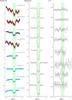 |
Fig. 5 Eight transit light curves of GJ 436b. The two upper panels are the data at 3.6 μm from 2009 January 9 and 28. The following two were taken at 4.5 μm on 2009 January 17 and 30. The lower four were obtained at 8 μm on 2007 June 29, 2008 July 12, 2009 January 25 and February 2. The left plot displays the raw binned and unbinned data, the middle one the binned data corrected for instrumental systematics, and the right one the binned residuals. Measurements are binned per interval of 7 min. The light curves are shifted along the y-axis for the sake of clarity. The shaded green areas show the transit events. |
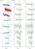 |
Fig. 6 Eight occultation light curves of GJ 436b. The two upper plots are the data at 3.6 μm from 2008 January 30 and 2011 February 1. The following two were obtained with the 4.5 μm channel on 2008 February 2 and 2011 January 24. The fifth is the light curve at 5.8 μm from 2008 February 5. The last three were taken at 8 μm on 2007 June 30, 2008 June 11, and 13. The left plot displays the raw data, the middle one the corrected data, and the right one the residuals. The shaded green areas show the eclipse events. |
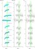 |
Fig. 7 Same as Fig. 6 with eight occultation light curves of GJ 436b at 8 μm. They were obtained respectively on 2008 June 16, 19, July 12, 14, 2009 January 27, 29, February 1 and 4. |
See Sect. 3.1.1 of the MIPS instrument handbook.
PyRAF is a command language for running IRAF tasks based on the Python scripting language.
IRAF is distributed by the National Optical Astronomy Observatory, which is operated by the Association of Universities for Research in Astronomy, Inc., under cooperative agreement with the National Science Foundation.
A 1-dimensional Gaussian of a given (fixed or pre-computed) FWHM is fitted to the marginal profiles in the x- and y-directions using non-linear least square techniques. Contrary to a 2D Gaussian fit it adjusts the PSF profile in both directions separately.
Because the fraction of the flux falling into a pixel at the edge of the aperture does not correspond to the fraction of the aperture within the same pixel, the measured flux on each pixel at the aperture border is wrongly evaluated.
See Sect. 4.4 and 4.5 of the Spitzer Observer’s Manual, and http://irsa.ipac.caltech.edu/data/SPITZER/docs/irac/warmfeatures/
Jump parameters are the model parameters that are randomly perturbed at each step of the MCMC.
Acknowledgments
This work is based in part on observations made with the Spitzer Space Telescope, which is operated by the Jet Propulsion Laboratory, California Institute of Technology under a contract with NASA. Support for this work was provided by NASA through an award issued by JPL/Caltech. M. Gillon is FNRS Research Associate. N. Astudillo acknowledges support from “Becas de Doctorado en el Extranjero, Becas Chile” (grant 72120460). V. Neves and N. C. Santos acknowledge the support by the European Research Council/European Community under the FP7 through Starting Grant agreement number 239953. NCS was also supported by FCT through the Investigador FCT contract reference IF/00169/2012 and POPH/FSE (EC) by FEDER funding through the programme “Programa Operacional de Factores de Competitividade – COMPETE”. We thank the anonymous referee for his helpful comments and suggestions as well as Pierre Drossart for helpful discussion about the methane fluorescence, Gwenaël Boué for information about ARoME use, Michael Line for providing his models from Moses et al. (2013), and Heather Knutson. We are grateful to Josefina Montalban for highlights on the stellar parameters and Thierry Morel for discussions about errors on inferred parameters for low mass stars. We thank Eva Eulaers, Alice Decock, and Sebastien Salmon for their helpful comments on the redaction. A special thank to Sandrine Sohy for her help and commitment in programming part of this work.
References
- Agol, E., Steffen, J., Sari, R., & Clarkson, W. 2005, MNRAS, 359, 567 [NASA ADS] [CrossRef] [Google Scholar]
- Agúndez, M., Venot, O., Selsis, F., & Iro, N. 2014, ApJ, 781, 68 [NASA ADS] [CrossRef] [Google Scholar]
- Alonso, R., Barbieri, M., Rabus, M., et al. 2008, A&A, 487, L5 [NASA ADS] [CrossRef] [EDP Sciences] [Google Scholar]
- Anglada-Escudé, G., & Butler, R. P. 2012, ApJS, 200, 15 [NASA ADS] [CrossRef] [Google Scholar]
- Anglada-Escudé, G., & Tuomi, M. 2012, A&A, 548, A58 [NASA ADS] [CrossRef] [EDP Sciences] [Google Scholar]
- Anglada-Escudé, G., Rojas-Ayala, B., Boss, A. P., Weinberger, A. J., & Lloyd, J. P. 2013, A&A, 551, A48 [NASA ADS] [CrossRef] [EDP Sciences] [Google Scholar]
- Baines, K. H., Mickelson, M. E., Larson, L. E., & Ferguson, D. W. 1995, Icarus, 114, 328 [NASA ADS] [CrossRef] [Google Scholar]
- Ballard, S., Charbonneau, D., Deming, D., et al. 2010a, PASP, 122, 1341 [NASA ADS] [CrossRef] [Google Scholar]
- Ballard, S., Christiansen, J. L., Charbonneau, D., et al. 2010b, ApJ, 716, 1047 [NASA ADS] [CrossRef] [Google Scholar]
- Bean, J. L., Benedict, G. F., Charbonneau, D., et al. 2008, A&A, 486, 1039 [NASA ADS] [CrossRef] [EDP Sciences] [Google Scholar]
- Bean, J. L., Désert, J.-M., Seifahrt, A., et al. 2013, ApJ, 771, 108 [NASA ADS] [CrossRef] [Google Scholar]
- Beaulieu, J. P., Carey, S., Ribas, I., & Tinetti, G. 2008, ApJ, 677, 1343 [NASA ADS] [CrossRef] [Google Scholar]
- Beaulieu, J.-P., Tinetti, G., Kipping, D. M., et al. 2011, ApJ, 731, 16 [NASA ADS] [CrossRef] [Google Scholar]
- Berta, Z. K., Irwin, J., Charbonneau, D., Burke, C. J., & Falco, E. E. 2012, AJ, 144, 145 [NASA ADS] [CrossRef] [Google Scholar]
- Beust, H., Bonfils, X., Montagnier, G., Delfosse, X., & Forveille, T. 2012, A&A, 545, A88 [NASA ADS] [CrossRef] [EDP Sciences] [Google Scholar]
- Bonfils, X., Delfosse, X., Udry, S., et al. 2005, A&A, 442, 635 [NASA ADS] [CrossRef] [EDP Sciences] [Google Scholar]
- Bonfils, X., Gillon, M., Udry, S., et al. 2012, A&A, 546, A27 [NASA ADS] [CrossRef] [EDP Sciences] [Google Scholar]
- Bonfils, X., Delfosse, X., Udry, S., et al. 2013, A&A, 549, A109 [NASA ADS] [CrossRef] [EDP Sciences] [Google Scholar]
- Boué, G., Montalto, M., Boisse, I., Oshagh, M., & Santos, N. C. 2013, A&A, 550, A53 [NASA ADS] [CrossRef] [EDP Sciences] [Google Scholar]
- Burrows, A., & Sharp, C. M. 1999, ApJ, 512, 843 [NASA ADS] [CrossRef] [Google Scholar]
- Butler, R. P., Vogt, S. S., Marcy, G. W., et al. 2004, ApJ, 617, 580 [NASA ADS] [CrossRef] [Google Scholar]
- Cáceres, C., Ivanov, V. D., Minniti, D., et al. 2009, A&A, 507, 481 [NASA ADS] [CrossRef] [EDP Sciences] [Google Scholar]
- Campo, C. J., Harrington, J., Hardy, R. A., et al. 2011, ApJ, 727, 125 [NASA ADS] [CrossRef] [Google Scholar]
- Casagrande, L., Flynn, C., & Bessell, M. 2008, MNRAS, 389, 585 [NASA ADS] [CrossRef] [MathSciNet] [Google Scholar]
- Charbonneau, D., Brown, T. M., Noyes, R. W., & Gilliland, R. L. 2002, ApJ, 568, 377 [NASA ADS] [CrossRef] [Google Scholar]
- Charbonneau, D., Allen, L. E., Megeath, S. T., et al. 2005, ApJ, 626, 523 [NASA ADS] [CrossRef] [Google Scholar]
- Charbonneau, D., Knutson, H. A., Barman, T., et al. 2008, ApJ, 686, 1341 [NASA ADS] [CrossRef] [MathSciNet] [Google Scholar]
- Charbonneau, D., Berta, Z. K., Irwin, J., et al. 2009, Nature, 462, 891 [NASA ADS] [CrossRef] [PubMed] [Google Scholar]
- Claret, A., & Bloemen, S. 2011, A&A, 529, A75 [NASA ADS] [CrossRef] [EDP Sciences] [Google Scholar]
- Coughlin, J. L., Stringfellow, G. S., Becker, A. C., et al. 2008, ApJ, 689, L149 [Google Scholar]
- Cowan, N. B., & Agol, E. 2011, ApJ, 726, 82 [Google Scholar]
- Croll, B., Lafreniere, D., Albert, L., et al. 2011, AJ, 141, 30 [NASA ADS] [CrossRef] [Google Scholar]
- Crossfield, I. J. M., Barman, T., Hansen, B. M. S., & Howard, A. W. 2013, A&A, 559, A33 [NASA ADS] [CrossRef] [EDP Sciences] [Google Scholar]
- Delfosse, X., Forveille, T., Perrier, C., & Mayor, M. 1998, A&A, 331, 581 [NASA ADS] [Google Scholar]
- Delfosse, X., Forveille, T., Ségransan, D., et al. 2000, A&A, 364, 217 [NASA ADS] [Google Scholar]
- Deming, D., Seager, S., Richardson, L. J., & Harrington, J. 2005, Nature, 434, 740 [NASA ADS] [CrossRef] [PubMed] [Google Scholar]
- Deming, D., Harrington, J., Laughlin, G., et al. 2007, ApJ, 667, L199 [NASA ADS] [CrossRef] [Google Scholar]
- Deming, D., Swain, M., Beichman, C., et al. 2009, in astro2010: The Astronomy and Astrophysics Decadal Survey, 62 [Google Scholar]
- Demory, B., Gillon, M., Barman, T., et al. 2007, A&A, 475, 1125 [NASA ADS] [CrossRef] [EDP Sciences] [Google Scholar]
- Demory, B.-O., Torres, G., Neves, V., et al. 2013, ApJ, 768, 154 [NASA ADS] [CrossRef] [Google Scholar]
- Désert, J., Lecavelier des Etangs, A., Hébrard, G., et al. 2009, ApJ, 699, 478 [NASA ADS] [CrossRef] [Google Scholar]
- Eastman, J., Siverd, R., & Gaudi, B. S. 2010, PASP, 122, 935 [NASA ADS] [CrossRef] [Google Scholar]
- Fazio, G. G., Hora, J. L., Allen, L. E., et al. 2004, ApJS, 154, 10 [NASA ADS] [CrossRef] [Google Scholar]
- Ford, E. B. 2006, ApJ, 642, 505 [NASA ADS] [CrossRef] [Google Scholar]
- Fortney, J. J. 2005, MNRAS, 364, 649 [NASA ADS] [CrossRef] [Google Scholar]
- Fortney, J. J., Sudarsky, D., Hubeny, I., et al. 2003, ApJ, 589, 615 [Google Scholar]
- Fortney, J. J., Marley, M. S., Lodders, K., Saumon, D., & Freedman, R. 2005, ApJ, 627, L69 [NASA ADS] [CrossRef] [Google Scholar]
- Fortney, J. J., Lodders, K., Marley, M. S., & Freedman, R. S. 2008, ApJ, 678, 1419 [NASA ADS] [CrossRef] [Google Scholar]
- Fortney, J. J., Shabram, M., Showman, A. P., et al. 2010, ApJ, 709, 1396 [NASA ADS] [CrossRef] [Google Scholar]
- Fortney, J. J., Mordasini, C., Nettelmann, N., et al. 2013, ApJ, 775, 80 [NASA ADS] [CrossRef] [Google Scholar]
- Freedman, R. S., Marley, M. S., & Lodders, K. 2008, ApJS, 174, 504 [NASA ADS] [CrossRef] [Google Scholar]
- Gardner, J. P., Mather, J. C., Clampin, M., et al. 2006, in SPIE Conf., 6265 [Google Scholar]
- Gelman, A., & Rubin, D. B. 1992, Stat. Science, 7, 457 [Google Scholar]
- Gideon, S. 1978, Ann. Stat., 6, 461 [NASA ADS] [CrossRef] [MathSciNet] [Google Scholar]
- Gillon, M., Pont, F., Moutou, C., et al. 2006, A&A, 459, 249 [NASA ADS] [CrossRef] [EDP Sciences] [Google Scholar]
- Gillon, M., Demory, B., Barman, T., et al. 2007a, A&A, 471, L51 [NASA ADS] [CrossRef] [EDP Sciences] [Google Scholar]
- Gillon, M., Magain, P., Chantry, V., et al. 2007b, in Transiting Extrapolar Planets Workshop, eds. C. Afonso, D. Weldrake, & T. Henning, ASP Conf. Ser., 366, 113 [Google Scholar]
- Gillon, M., Pont, F., Demory, B., et al. 2007c, A&A, 472, L13 [NASA ADS] [CrossRef] [EDP Sciences] [Google Scholar]
- Gillon, M., Demory, B., Triaud, A. H. M. J., et al. 2009, A&A, 506, 359 [NASA ADS] [CrossRef] [EDP Sciences] [Google Scholar]
- Gillon, M., Lanotte, A. A., Barman, T., et al. 2010, A&A, 511, A3 [NASA ADS] [CrossRef] [EDP Sciences] [Google Scholar]
- Gillon, M., Triaud, A. H. M. J., Fortney, J. J., et al. 2012, A&A, 542, A4 [NASA ADS] [CrossRef] [EDP Sciences] [Google Scholar]
- Giménez, A. 2006, ApJ, 650, 408 [NASA ADS] [CrossRef] [Google Scholar]
- Hauschildt, P. H., Allard, F., Ferguson, J., Baron, E., & Alexander, D. R. 1999, ApJ, 525, 871 [NASA ADS] [CrossRef] [Google Scholar]
- Holman, M. J., & Murray, N. W. 2005, Science, 307, 1288 [NASA ADS] [CrossRef] [PubMed] [Google Scholar]
- Holman, M. J., Winn, J. N., Latham, D. W., et al. 2006, ApJ, 652, 1715 [NASA ADS] [CrossRef] [Google Scholar]
- Houck, J. R., Roellig, T. L., van Cleve, J., et al. 2004, ApJS, 154, 18 [NASA ADS] [CrossRef] [Google Scholar]
- Howarth, I. D., Siebert, K. W., Hussain, G. A. J., & Prinja, R. K. 1997, MNRAS, 284, 265 [NASA ADS] [CrossRef] [Google Scholar]
- Johnson, J. A., & Apps, K. 2009, ApJ, 699, 933 [NASA ADS] [CrossRef] [Google Scholar]
- Kane, S. R., & Gelino, D. M. 2010, ApJ, 724, 818 [NASA ADS] [CrossRef] [Google Scholar]
- Kass, R. E., & Raftery, A. E. 1995, J. Am. Stat. Assoc., 90, 773 [Google Scholar]
- Kipping, D. M. 2009, MNRAS, 392, 181 [NASA ADS] [CrossRef] [Google Scholar]
- Knutson, H. A., Charbonneau, D., Allen, L. E., Burrows, A., & Megeath, S. T. 2008, ApJ, 673, 526 [NASA ADS] [CrossRef] [Google Scholar]
- Knutson, H. A., Charbonneau, D., Burrows, A., O’Donovan, F. T., & Mandushev, G. 2009a, ApJ, 691, 866 [NASA ADS] [CrossRef] [Google Scholar]
- Knutson, H. A., Charbonneau, D., Cowan, N. B., et al. 2009b, ApJ, 690, 822 [NASA ADS] [CrossRef] [Google Scholar]
- Knutson, H. A., Madhusudhan, N., Cowan, N. B., et al. 2011, ApJ, 735, 27 [NASA ADS] [CrossRef] [Google Scholar]
- Knutson, H. A., Benneke, B., Deming, D., & Homeier, D. 2014, Nature, 505, 66 [NASA ADS] [CrossRef] [Google Scholar]
- Kovács, G., Zucker, S., & Mazeh, T. 2002, A&A, 391, 369 [NASA ADS] [CrossRef] [EDP Sciences] [Google Scholar]
- Kozai, Y. 1962, AJ, 67, 591 [Google Scholar]
- Krist, J. 2002, Tiny Tim/SIRTF User’s Guide (Pasadena: SSC) [Google Scholar]
- Kulow, J. R., France, K., Linsky, J., & Parke Loyd, R. O. 2014, ApJ, 786, 132 [NASA ADS] [CrossRef] [Google Scholar]
- Kürster, M., Endl, M., Rouesnel, F., et al. 2003, A&A, 403, 1077 [NASA ADS] [CrossRef] [EDP Sciences] [Google Scholar]
- Leggett, S. K. 1992, ApJS, 82, 351 [NASA ADS] [CrossRef] [Google Scholar]
- Letawe, Y., Magain, P., Letawe, G., Courbin, F., & Hutsemékers, D. 2008, ApJ, 679, 967 [Google Scholar]
- Lewis, N. K., Showman, A. P., Fortney, J. J., et al. 2010, ApJ, 720, 344 [NASA ADS] [CrossRef] [Google Scholar]
- Lewis, N. K., Knutson, H. A., Showman, A. P., et al. 2013, ApJ, 766, 95 [NASA ADS] [CrossRef] [Google Scholar]
- Line, M. R., Zhang, X., Vasisht, G., et al. 2012, ApJ, 749, 93 [NASA ADS] [CrossRef] [Google Scholar]
- Line, M. R., Wolf, A. S., Zhang, X., et al. 2013, ApJ, 775, 137 [NASA ADS] [CrossRef] [Google Scholar]
- Line, M. R., Knutson, H., Wolf, A. S., & Yung, Y. L. 2014, ApJ, 783, 70 [NASA ADS] [CrossRef] [Google Scholar]
- Lodders, K. 2003, ApJ, 591, 1220 [NASA ADS] [CrossRef] [Google Scholar]
- Lodders, K., & Fegley, B. 2002, Icarus, 155, 393 [NASA ADS] [CrossRef] [Google Scholar]
- Madhusudhan, N., & Seager, S. 2011, ApJ, 729, 41 [NASA ADS] [CrossRef] [Google Scholar]
- Madhusudhan, N., Knutson, H., Fortney, J., & Barman, T. 2014, Protostars and Planets VI, eds. H. Beuther, R. Klessen, C. Dullemond, & Th. Henning, submitted [arXiv:1402.1169] [Google Scholar]
- Magain, P., Courbin, F., & Sohy, S. 1998, ApJ, 494, 472 [NASA ADS] [CrossRef] [Google Scholar]
- Magain, P., Courbin, F., Gillon, M., et al. 2007, A&A, 461, 373 [NASA ADS] [CrossRef] [EDP Sciences] [Google Scholar]
- Mandel, K., & Agol, E. 2002, ApJ, 580, L171 [NASA ADS] [CrossRef] [Google Scholar]
- Maness, H. L., Marcy, G. W., Ford, E. B., et al. 2007, PASP, 119, 90 [NASA ADS] [CrossRef] [Google Scholar]
- Mayor, M., Pepe, F., Queloz, D., et al. 2003, The Messenger, 114, 20 [NASA ADS] [Google Scholar]
- Moses, J. I., Line, M. R., Visscher, C., et al. 2013, ApJ, 777, 34 [NASA ADS] [CrossRef] [Google Scholar]
- Neves, V., Bonfils, X., Santos, N. C., et al. 2012, A&A, 538, A25 [NASA ADS] [CrossRef] [EDP Sciences] [Google Scholar]
- Neves, V., Bonfils, X., Santos, N. C., et al. 2013, A&A, 551, A36 [NASA ADS] [CrossRef] [EDP Sciences] [Google Scholar]
- Ofir, A. 2014, A&A, 561, A138 [NASA ADS] [CrossRef] [EDP Sciences] [Google Scholar]
- Pepe, F., Lovis, C., Ségransan, D., et al. 2011, A&A, 534, A58 [NASA ADS] [CrossRef] [EDP Sciences] [Google Scholar]
- Pont, F., Gilliland, R. L., Knutson, H., Holman, M., & Charbonneau, D. 2009, MNRAS, 393, L6 [NASA ADS] [CrossRef] [Google Scholar]
- Pont, F., Zucker, S., & Queloz, D. 2006, MNRAS, 373, 231 [NASA ADS] [CrossRef] [Google Scholar]
- Queloz, D., Eggenberger, A., Mayor, M., et al. 2000, A&A, 359, L13 [NASA ADS] [Google Scholar]
- Reach, W. T., Megeath, S. T., Cohen, M., et al. 2005, PASP, 117, 978 [NASA ADS] [CrossRef] [Google Scholar]
- Ribas, I., Font-Ribera, A., & Beaulieu, J. 2008, ApJ, 677, L59 [NASA ADS] [CrossRef] [MathSciNet] [Google Scholar]
- Ribas, I., Font-Ribera, A., Beaulieu, J., Morales, J. C., & García-Melendo, E. 2009, in IAU Symp., 253, 149 [Google Scholar]
- Rieke, G. H., Young, E. T., Engelbracht, C. W., et al. 2004, ApJS, 154, 25 [NASA ADS] [CrossRef] [Google Scholar]
- Russell, H. N. 1916, ApJ, 43, 173 [NASA ADS] [CrossRef] [Google Scholar]
- Schlaufman, K. C., & Laughlin, G. 2010, A&A, 519, A105 [NASA ADS] [CrossRef] [EDP Sciences] [Google Scholar]
- Seager, S. 2010, Exoplanet Atmospheres: Physical Processes (Princeton University Press) [Google Scholar]
- Seager, S., & Deming, D. 2010, ARA&A, 48, 631 [NASA ADS] [CrossRef] [Google Scholar]
- Seager, S., & Mallén-Ornelas, G. 2003, ApJ, 585, 1038 [NASA ADS] [CrossRef] [Google Scholar]
- Seager, S., Deming, D., & Valenti, J. A. 2009, Transiting Exoplanets with JWST, eds. H. A. Thronson, M. Stiavelli, & A. Tielens (Springer), 123 [Google Scholar]
- Selsis, F., Kasting, J. F., Levrard, B., et al. 2007, A&A, 476, 1373 [NASA ADS] [CrossRef] [EDP Sciences] [Google Scholar]
- Shabram, M., Fortney, J. J., Greene, T. P., & Freedman, R. S. 2011, ApJ, 727, 65 [NASA ADS] [CrossRef] [Google Scholar]
- Shporer, A., Mazeh, T., Pont, F., et al. 2009, ApJ, 694, 1559 [NASA ADS] [CrossRef] [Google Scholar]
- Spada, F., Demarque, P., Kim, Y. C., & Sills, A. 2013, ApJ, 776, 87 [NASA ADS] [CrossRef] [Google Scholar]
- Stetson, P. B. 1987, PASP, 99, 191 [NASA ADS] [CrossRef] [Google Scholar]
- Stevenson, K. B., Harrington, J., Nymeyer, S., et al. 2010, Nature, 464, 1161 [NASA ADS] [CrossRef] [PubMed] [Google Scholar]
- Stevenson, K. B., Harrington, J., Fortney, J. J., et al. 2012a, ApJ, 754, 136 [NASA ADS] [CrossRef] [Google Scholar]
- Stevenson, K. B., Harrington, J., Lust, N. B., et al. 2012b, ApJ, 755, 9 [NASA ADS] [CrossRef] [Google Scholar]
- Sudarsky, D., Burrows, A., Hubeny, I., & Li, A. 2005, ApJ, 627, 520 [NASA ADS] [CrossRef] [Google Scholar]
- Tinetti, G., Vidal-Madjar, A., Liang, M., et al. 2007, Nature, 448, 169 [NASA ADS] [CrossRef] [PubMed] [Google Scholar]
- Torres, G. 2007, ApJ, 671, L65 [NASA ADS] [CrossRef] [Google Scholar]
- Torres, G. 2013, Astron. Nachr., 334, 4 [NASA ADS] [CrossRef] [Google Scholar]
- Venot, O., Agúndez, M., Selsis, F., Tessenyi, M., & Iro, N. 2014, A&A, 562, A51 [NASA ADS] [CrossRef] [EDP Sciences] [Google Scholar]
- von Braun, K., Boyajian, T. S., Kane, S. R., et al. 2012, ApJ, 753, 171 [NASA ADS] [CrossRef] [Google Scholar]
- Waldmann, I. P., Tinetti, G., Drossart, P., et al. 2012, ApJ, 744, 35 [NASA ADS] [CrossRef] [Google Scholar]
- Werner, M. W., Roellig, T. L., Low, F. J., et al. 2004, ApJS, 154, 1 [Google Scholar]
- Winn, J. N. 2010, in Exoplanet, ed. S. Seager (University of Arizona Press), 55 [Google Scholar]
- Zucker, S., & Mazeh, T. 2006, MNRAS, 371, 1513 [NASA ADS] [CrossRef] [Google Scholar]
All Tables
System parameters derived from our global analysis of the Spitzer data and radial velocities.
Individual measurements of the occultation depths for the different AORs (Sect. 3.4.3).
All Figures
|
Fig. 1 Secondary eclipses of GJ 436b observed with the IRS (top) and MIPS (bottom) instruments. Relative flux offsets are applied to datasets for clarity. On the left, raw data are represented by cyan dots for the unbinned data and by black dots for binned data per interval of 7 min with their error bars. The superimposed red line is the best-fitting model and includes the transit model. On the middle, the same binned data divided by the best-fitting baseline model reveal the occultation shape. The eclipse model is superposed in red. The right panel displays the binned residuals from the same dataset. The shaded green area of every panel shows the eclipse event. |
| In the text | |
|
Fig. 2 Evolution of the photometric precision for raw data with the aperture radius according to different centring techniques in a complete dataset (e.g., AOR: 42614016). The 2D Gaussian adjustment (green asterisks) provides the best photometric precision for raw data in comparison to a centroid fit (magenta crosses), a double 1D Gaussian fit from the previously computed x- or y-FWHM (cyan boxes and red diamonds respectively), and a 1D Gaussian fit with a fixed FWHM (blue stars), in particular for small aperture radii. |
| In the text | |
|
Fig. 3 For illustration, evolution of the parameters measured by our reduction pipeline for a randomly chosen IRAC dataset (at 3.6 μm, 2009 January 9, AOR: 28894208). From top to bottom and left to right we display the evolutions of the normalised stellar fluxes, the PSF x- and y-centres, the background values, and the PSF FWHMs in the x- and y-directions. The last three panels display the correlation diagrams for several parameters, revealing a clear dependence on the FWHM with the position for both directions. The first values (thick cyan coloured dots) are rejected, as the measured parameters (e.g., sky contribution) are not yet stabilised. |
| In the text | |
|
Fig. 4 Stellar flux evolution in the 3.6 (top), 4.5 (middle), and 8.0 μm (bottom) IRAC channels. The stellar flux slightly fluctuates with time in the 3.6 and 4.5 μm bandpasses, and is constant at 8.0 μm. A different inter-pixel map is used for the Warm mission data. The Warm Spitzer phase is shaded in pale pink for clarity. The flux modulation is probably due to the uncorrected intra-pixel effect and to the calibration uncertainties, which are not displayed here for clarity. |
| In the text | |
|
Fig. 8 Top: radial velocities measured with the HIRES and HARPS spectrographs. The data are period-folded on the best-fit transit ephemeris, the 0 of the x-axis corresponding to the inferior conjunction time. The fit is superimposed on red and the respective residuals are shown on the bottom panel. The left panels display those corresponding data during the whole planetary orbit and the right ones are a zoom on the box to highlight the (undetected) Rossiter-McLaughlin effect. The HARPS binned data are added in black diamonds filled white for clarity. |
| In the text | |
|
Fig. 9 Detrended Spitzer 3.6 μm (left), 4.5 μm (middle), and 8 μm (right) photometry folded on the best-fit transit ephemeris obtained in our analysis per channel for the transits (top, Sect. 3.4.3) and in our global analysis for the occultations (bottom). The best-fit eclipse models are superimposed. |
| In the text | |
|
Fig. 10 Occultation depth variation at 8 μm as function of time. Brown diamonds with their 1σ-error bar represents occultation depths. The dashed blue lines indicate temporal caesura in the x-axis. The red horizontal line displays the eclipse depth value obtained during the global analysis and the shaded region surrounding it is its 1σ-error bar. |
| In the text | |
|
Fig. 11 Transit parameter variations. From top to bottom, the plots respectively show the transit depth, the transit duration, and the transit timing variation with their error bars according to time for the different IRAC channels. The pink dots stand for the 3.6 μm channel, the green crosses for the 4.5 μm channel, and the brown diamonds for the 8 μm channel. The vertical dashed blue lines indicate temporal caesura in the x-axis. The horizontal red lines present in the two top panels respectively indicate the transit depth and duration derived from the global analysis. The shaded surrounding area is its 1σ error bar. |
| In the text | |
|
Fig. 12 Influence of the chosen aperture radius and the baseline modelling. We present the same light curve (at 3.6 μm, 2008 January 30, AOR: 24882688) four times, however showing different noise level and a different occultation depth due to the data reduction and analysis. On the left, the aperture photometry is centred by a 2D elliptical Gaussian fit with an aperture radius of 1.9 pixels, while on the right the aperture radius equals 3.5 pixels. They all proceed to the same MCMC analysis with the inferred parameters from Table 3, except that the top ones contain a baseline model dealing with the measured PSF FWHM, while the bottom ones do not. |
| In the text | |
|
Fig. 13 Flux modulations present in the 2010 June 6 Spitzer light curve (AOR: 38807296) during GJ 436 monitoring. |
| In the text | |
|
Fig. 14 Lack of correlation on the PSF FWHM of GJ 436 (AOR: 38807296) with the square root of the pixel noise parameter ( |
| In the text | |
|
Fig. 15 Transit-like structures detected in two residual light curves by our own version of the code MISS MarPLE (Berta et al. 2012). For both structures, a box-like model illustrates a transit depth of 120 ppm and a duration of 0.6 h. |
| In the text | |
|
Fig. 16 Top: timing of GJ 436 observations with the 3.6 and 4.5 μm IRAC channels. The two vertical lines indicate the datasets having the transit-like features. Bottom: distribution of the possible period range for the putative additive transiting planet. The observational coverage discards all periods below 1.18 days. |
| In the text | |
|
Fig. 17 Atypical behaviour of measured parameters during two of S12’s UCF-1.01 transits. Left panel: background contribution discontinuity around BJD 2 455 225.09. Right panel: points out a strong fluctuation of the x-FWHM around BJD 2 454 662.32. UCF-1.01 transit events are shaded in green. |
| In the text | |
|
Fig. 18 Highlight on the impact of the data reduction/analysis details on the presence of low-amplitude transit-shaped structures in the Spitzer photometry (2010 Jan. 28, AOR: 38702848). We apply relative flux offsets in the above two plots for clarity. The upper dataset is the result of aperture photometry with a 2D elliptical Gaussian centring while the lower one is done with a double 1D Gaussian fit. The upper is corrected with a baseline involving the measured FWHM while the lower is not. Black dots are the binned data per interval of 5 min with 1σ error bars. The supposed UCF-1.01 (right) and UCF-1.02 (left) transit events are shaded in green. |
| In the text | |
|
Fig. 19 Same as Fig. 18 for the 2011 Jul 30 data (AOR: 42614016). The upper dataset is the result of aperture photometry with a 2D elliptical Gaussian centring and is corrected for all systematics minimising the BIC. The lower dataset is produced from a double 1D Gaussian fit of the computed x-FWHM and corrected in the same way. The shaded green area corresponds to UCF-1.01 transit event. |
| In the text | |
|
Fig. 20 GJ 436 periodogram of the residuals for the model composed of 1 planet on a Keplerian orbit plus 1 drift. The horizontal yellow line represents the 1% false alarm probability. No peak shows a significant power excess. |
| In the text | |
|
Fig. 21 Conservative detection limits on Mpsini applied to GJ 436 residual RV time-series around a chosen model (composed of planets, linear drifts, and/or a simple sine function). Planets above the limit are excluded, with a 99% confidence level, for all 12 trial phases. The vertical dashed yellow line marks the duration of the survey. |
| In the text | |
|
Fig. 22 Model planet-to-star flux ratios compared to the observed Spitzer occultation data. Both models assume a hot day side, with absorbed energy redistributed only over the dayside. The blue model uses solar metallicity, while the red model uses 50×-solar. The Spitzer data are orange circle while the model band averages in the six bands are shown as coloured squares. The location of prominent absorption features that differ between the models (where CO and CO2 absorb strongly) are labelled. The planet-to-star flux ratios of 500, 700, and 900 K blackbodies are shown in dashed black. |
| In the text | |
|
Fig. 23 Comparison of our observed Spitzer occultation data with synthetic emission spectra for GJ 436b from Moses et al. (2013). The green and blue curves correspond respectively to the best fit retrieved model, given S10 data, using the method of Line et al. and the 300×-solar model. The model band averages in the six bands are shown as coloured squares. Our Spitzer data are shown as orange circles. |
| In the text | |
|
Fig. 24 Model transit radius as function of wavelength compared with published transit depths and our Spitzer results. From left to right, the radii are derived from EPOXI (Ballard et al. 2010b), HST WFC3 (represented by empty diamonds with thinner error bars in the 1.14–1.65 μm wavelength range, Knutson et al. 2014), HST NICMOS (Pont et al. 2009), the H and K bands from the ground (Alonso et al. 2008; Cáceres et al. 2009), and IRAC (ours) studies. Three models are shown. In orange is the 50×-solar model from Fig. 22. In red and blue are transmission spectra taken from Shabram et al. (2011), who used mixing ratios suggested for the planetary dayside by S10. Band-average calculations are shown as squares for the three models, across the Spitzer bandpasses. The dramatic differences between the models at optical wavelength are only due to different assumptions about the abundances of alkali metals. The blue and red models, which have depleted CH4, and enhanced CO and CO2, are generally preferred. |
| In the text | |
|
Fig. 25 Top: the observed phase curve of GJ 436 at 8 μm (2008 July 12, AORs: 27863296, 27863552, 27863808) superimposed to a model for a Lambert sphere (red line). The adopted baseline models are respectively p([xy] |
| In the text | |
|
Fig. 26 Theoretical effective temperature-mass relations from the stellar evolution model of Spada et al. (2013), with the mixing length parameter α set to 0.5. Theoretical 4 Gyr isochrones are plotted for different metallicities indicated by legend. The magenta filled box shows the GJ 436 position on the diagram according to von Braun et al. (2012)’s stellar temperature and our inferred stellar mass. |
| In the text | |
|
Fig. 5 Eight transit light curves of GJ 436b. The two upper panels are the data at 3.6 μm from 2009 January 9 and 28. The following two were taken at 4.5 μm on 2009 January 17 and 30. The lower four were obtained at 8 μm on 2007 June 29, 2008 July 12, 2009 January 25 and February 2. The left plot displays the raw binned and unbinned data, the middle one the binned data corrected for instrumental systematics, and the right one the binned residuals. Measurements are binned per interval of 7 min. The light curves are shifted along the y-axis for the sake of clarity. The shaded green areas show the transit events. |
| In the text | |
|
Fig. 6 Eight occultation light curves of GJ 436b. The two upper plots are the data at 3.6 μm from 2008 January 30 and 2011 February 1. The following two were obtained with the 4.5 μm channel on 2008 February 2 and 2011 January 24. The fifth is the light curve at 5.8 μm from 2008 February 5. The last three were taken at 8 μm on 2007 June 30, 2008 June 11, and 13. The left plot displays the raw data, the middle one the corrected data, and the right one the residuals. The shaded green areas show the eclipse events. |
| In the text | |
|
Fig. 7 Same as Fig. 6 with eight occultation light curves of GJ 436b at 8 μm. They were obtained respectively on 2008 June 16, 19, July 12, 14, 2009 January 27, 29, February 1 and 4. |
| In the text | |
Current usage metrics show cumulative count of Article Views (full-text article views including HTML views, PDF and ePub downloads, according to the available data) and Abstracts Views on Vision4Press platform.
Data correspond to usage on the plateform after 2015. The current usage metrics is available 48-96 hours after online publication and is updated daily on week days.
Initial download of the metrics may take a while.