| Issue |
A&A
Volume 570, October 2014
|
|
|---|---|---|
| Article Number | A57 | |
| Number of page(s) | 9 | |
| Section | Atomic, molecular, and nuclear data | |
| DOI | https://doi.org/10.1051/0004-6361/201424252 | |
| Published online | 16 October 2014 | |
Relevance of the H2 + O reaction pathway for the surface formation of interstellar water
Combined experimental and modeling study
1
Raymond and Beverly Sackler Laboratory for Astrophysics, Leiden
Observatory, University of Leiden,
PO Box 9513,
2300 RA
Leiden,
The Netherlands
e-mail:
lamberts@strw.leidenuniv.nl
2
Faculty of Science, Radboud University Nijmegen, IMM,
PO Box 9010, 6500 GL
Nijmegen, The
Netherlands
3
Division of Geological and Planetary Sciences, California
Institute of Technology, 1200 E.
California Blvd., Pasadena, California
91125,
USA
Received: 22 May 2014
Accepted: 9 September 2014
The formation of interstellar water is commonly accepted to occur on the surfaces of icy dust grains in dark molecular clouds at low temperatures (10–20 K), involving hydrogenation reactions of oxygen allotropes. As a result of the large abundances of molecular hydrogen and atomic oxygen in these regions, the reaction H2 + O has been proposed to contribute significantly to the formation of water as well. However, gas-phase experiments and calculations, as well as solid-phase experimental work contradict this hypothesis. Here, we use precisely executed temperature-programmed desorption (TPD) experiments in an ultra-high vacuum setup combined with kinetic Monte Carlo simulations to establish an upper limit of the water production starting from H2 and O. These reactants were brought together in a matrix of CO2 in a series of (control) experiments at different temperatures and with different isotopological compositions. The water detected with the quadrupole mass spectrometer upon TPD was found to originate mainly from contamination in the chamber itself. However, if water is produced in small quantities on the surface through H2 + O, this can only be explained by a combined classical and tunneled reaction mechanism. An absolutely conservative upper limit for the reaction rate was derived with a microscopic kinetic Monte Carlo model that converts the upper limit into the highest possible reaction rate. Incorporating this rate into simulation runs for astrochemically relevant parameters shows that the upper limit to the contribution of the reaction H2 + O in OH, and hence water formation, is 11% in dense interstellar clouds. Our combined experimental and theoretical results indicate, however, that this contribution is most likely much lower.
Key words: astrochemistry / molecular processes / ISM: clouds / methods: laboratory: solid state
© ESO, 2014
1. Introduction
The formation of interstellar water is commonly believed to occur mostly on the surfaces of icy dust grains in dark molecular clouds where the temperatures typically range between 10 and 20 K. In recent years, several studies have been focusing on the reaction of atomic hydrogen with O, O2, and O3 in interstellar ice analogs, both experimentally and through surface models (Hiraoka et al. 1998; Dulieu et al. 2010; Miyauchi et al. 2008; Ioppolo et al. 2008, 2010; Oba et al. 2009; Cuppen et al. 2010; Mokrane et al. 2009; Romanzin et al. 2011; Oba et al. 2012; Lamberts et al. 2013). A possibly interesting alternative pathway to form water under interstellar conditions starts from the reaction  and is followed by
  or
or  Reaction R1 has been proposed to contribute significantly to the formation of water since molecular hydrogen and atomic oxygen are both abundantly present in the dense regions of the interstellar medium (Cazaux et al. 2010, 2011). Additionally, Cazaux et al. (2010) proposed this reaction to be important for deuterium enrichment during water formation. Conceptually, the interaction between H2 and the surface could aid in breaking the H-H bond. The reaction is, however, endothermic by 960 K, making it intuitively unlikely to occur in the low-temperature regime. Moreover, a theoretical barrier in the gas phase of approximately 7000 K is predicted for the case that both O and H2 are in the ground state (Rogers et al. 2000). Gas-phase experimental work also predicts high barriers (~3000 K), as reviewed by Baulch et al. (1992). Barriers of this order of magnitude lead to thermally induced reaction rates that are so slow that their contribution to the full chemical reaction network becomes negligible even over the long interstellar timescales of several million years (Bergin & Tafalla 2007). It should be noted that at low temperatures tunneling may play an important role, but tunneling through the barrier of an endothermic reaction can only take place if the reactants have an initial energy equal to or higher than the endothermicity (Arnaut et al. 2006).
For these reasons, reaction R1 was excluded in the reaction scheme used by Cuppen & Herbst (2007), who studied the formation of ice mantles on interstellar grains. Recent solid-state laboratory studies by Oba et al. (2012) showed no detectable production of H2O by means of infrared spectroscopy upon co-deposition of H2 and O atoms, which motivated Taquet et al. (2013) to exclude it from their ice chemistry reaction network as well.
Here ultra-high vacuum (UHV) surface chemistry experiments are carried out at low temperature in conjunction with kinetic Monte Carlo modeling to clarify the ambiguity in the importance of the reaction H2 + O under interstellar conditions.
2. Calculation of the reaction rate
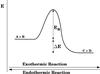 |
Fig. 1 Schematic representation of the energy level diagram of an exothermic and endothermic reaction. |
Reactions are often considered to take place along pathways such as those shown in Fig. 1. The reaction coordinate is depicted on the horizontal axis, energy on the vertical axis, ΔE indicates the difference in potential energy between reactants (A + B) and products (C + D), and the reaction rate is determined by the barrier or activation energy, Ea. In astrochemical models it is common to use a straightforward expression to calculate a reaction rate as a result of the large chemical networks involved (Garrod & Herbst 2006). Calculating the reaction rates therefore often involves a rather arbitrary choice between the expression for classically (i.e., thermally) activated reactions 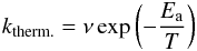 (1)and the expression for tunneling of a free particle through a rectangular barrier (Bell 1980)
 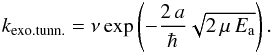 (2)Typically, the trial frequency ν is approximated by the standard value for physisorbed species, kT/h ≈ 1012 s-1 and a barrier width a of 1 Å is chosen. In the expression for the tunneling rate the reduced mass, μred, is usually taken to be the reduced mass of the total reacting system without taking into account the mutual orientation of the reactants. The mass should, however, be affiliated with the reaction coordinate involved, as was done in recent work of a linear bimolecular atom-transfer reaction leading to an effective mass, μeff (Oba et al. 2012). In the case of reaction R1 the difference between the reduced and the effective mass gives rise to a substantial increase of the reaction rate (see also Table 1).
Tunneling rates for endothermic reactions, kendo.tunn. (see Fig. 1), need to be calculated as a combination of Eqs. (1) and (2), where the classical contribution accounts for the part of the reaction barrier that lies below the endothermicity and the tunneled contribution for that above (Arnaut et al. 2006). This can be derived from arguments of detailed balance (or microscopic reversibility): in equilibrium the net flux between every pair of states is zero. The reaction rates should then obey the condition 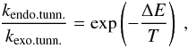 (3)and hence, following the definition for Ea from Fig. 1,
 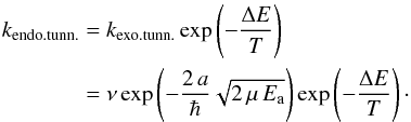 (4)The comparison between these various ways of calculating the reaction rate spans a wide range. as outlined in Table 1. A more accurate way to calculate reaction rates also takes into account the shape of the barrier, examples of which are the usage of the Eckart model by Taquet et al. (2013) or the implementation of instanton theory by Andersson et al. (2011). This results in modified tunneling reaction rates with differences of up to several orders of magnitude. Depending on the expression used, the resulting reaction rate can be substantially different. The ambiguity makes it hard to interpret these values in terms of their astronomical relevance. One way to partially circumvent this is to make use of upper (or lower) limits, determined experimentally.
In the following sections we use laboratory experiments combined with microscopic kinetic Monte Carlo simulations to constrain the reaction rate of reaction R1. Subsequently, the resulting reaction rate is incorporated into the same kinetic Monte Carlo model, but run with physical parameters relevant to the interstellar medium to test its astronomical significance.
Calculated reaction rates for the reaction H2 + O assuming classical and tunneled contributions.
List of (control) experiments and integrated baseline-corrected QMS signals for m/z = 20 and 22, i.e. H O and DO, and the calculated HO abundance in ML.
3. Experiments
3.1. Methods
Experiments were performed using the SURFRESIDE2 setup, which allows for the systematic investigation of solid-state reactions leading to the formation of molecules of astrophysical interest at cryogenic temperatures. SURFRESIDE2 consists of three UHV chambers with a room-temperature base-pressure between 10-9 − 10-10 mbar. The setup has already been extensively described in Ioppolo et al. (2013) and therefore only a brief description of the procedure is given here. A rotatable gold-coated copper substrate in the center of the main chamber is cooled to 13.5–14.0 K using a He closed-cycle cryostat with an absolute temperature accuracy of ≤2 K. This temperature is around the lower limit of what can be reached under our experimental conditions and was chosen to minimize the diffusion of the oxygen atoms, and simultaneously have a long lifetime of H2 and O on the surface. To study the solid-state reaction pathway H2 + O, the reactants need to be deposited on a surface while simultaneously preventing the competing reactions O + O → O2 and O + O2→ O3. This was achieved by using a matrix consisting of CO2 molecules and an overabundance of molecular hydrogen. A full experiment starts with the preparation of all selected gases in separate pre-pumped (≤10-5 mbar) dosing lines. Then a co-deposition of H2, O and CO2 is performed. Room-temperature carbon dioxide (Praxair 99.996%) is deposited through a metal deposition line under an angle of 90°. Room-temperature molecular hydrogen (Praxair 99.999%) is deposited on the surface through an UHV beam line with an angle of 45° with respect to the surface. Oxygen atoms are generated from 18O2 (Aldrich 99%) in another UHV beam line in a microwave plasma atom source (Oxford Scientific Ltd, see Anton et al. 2000) with an angle of 135° with respect to the surface. A custom-made nose-shaped quartz-pipe is placed in between the atom sources and the substrate. The pipe is designed in such a way that all chemically active species that are in their electronic and/or ro-vibrationally excited states are quenched to room temperature before being deposited to the surface. In addition to 18O atoms a (large) fraction of non-dissociated 18O2 is also present in the beam. The UHV beam lines can be operated independently and are separated from the main chamber by metal shutters. All experiments and the corresponding atomic and molecular fluxes are listed in Table 2. The effective O flux determination by Ioppolo et al. (2013) was repeated and found to be reproducible: 2 × 10¹¹ at cm-2 s-1 (uncertainty ~30%). Each (control) experiment was performed for 75 min. Experiments 1–3 were performed twice to check their reproducibility. The aim of these experiments is to determine an upper limit for the production of water during co-deposition.
SURFRESIDE2 has two main analytical tools: i) the ice composition is monitored in situ by means of reflection absorption infrared spectroscopy (RAIRS) in the range between 4000 and 700 cm-1 with a spectral resolution of 1 cm-1; ii) the main chamber gas-phase composition is monitored by a quadrupole mass spectrometer (QMS) that is placed behind the rotatable substrate. Here, we deposited a total of 0.9 ML O atoms per experiment, meaning that RAIRS could only be used if the reaction is indeed as efficient as claimed by the exothermic tunneled rate. RAIR difference spectra with respect to the bare substrate were recorded every 5 min, averaging over 512 scans. After the co-deposition was finished, the sample was rotated to face the QMS and a temperature-programmed desorption (TPD) experiment at 1 K min-1 was performed to monitor the desorption of the ice constituents. The QMS is typically used for the study of species that fall below the detection limit of RAIRS, that is, submonolayer experiments.
To convert the integrated area of the current (pressure) read by the QMS to a number of molecules desorbing from the sample, we performed several calibration experiments. First, to relate the ice thickness to a QMS signal, we deposited layers of water of three different thicknesses at 13.5–14 K, followed by a TPD at the usual ramp of 1 K min-1. Following this, the water RAIRS signal at 3280 and 1660 cm-1 of these three experiments was converted into a number of monolayers using the IR bandstrength. This is, however, not trivial because of the reflection mode of the IR spectrometer, which is setup dependent. The bandstrength of CO2 in reflection mode was determined through an isothermal desorption experiment by Ioppolo et al. (2013). A similar calibration experiment cannot be easily performed for H2O, because of the rearrangement of hydrogen bonds at high temperatures, which changes the desorption profile. Therefore, the ratio between the transmission bandstrengths of CO2 and H2O was taken from Gerakines et al. (1995) to derive the bandstrengths in reflection mode for the 3280 and 1660 cm-1 bands of water. Finally, the value for the integrated QMS signal, corresponding to one monolayer of desorbing water molecules, is determined by averaging over the three deposited water layers.
The experiments were analyzed by first performing a linear baseline correction between 115 and 195 K. Then, the mass 20 amu signal was integrated over two ranges; one centered on the CO2 desorption (~80 K) and one at the H2O desorption (~140 K) given in Table 2. The combined signal was converted into a number of produced monolayers, and given in the last column of Table 2.
In previous experiments not listed in Table 2, we used a different CO2 flux and another source of atomic oxygen, N O. The latter has the main advantage that the competing ozone channel is less likely to occur since there is only little O2 present in the plasma source. It does yield regular water (HO), which is hard to distinguish from the contamination present in all parts of the experimental setup. The use of 18O2 as a precursor of atomic oxygen would lead to the formation of HO, which can be better distinguished from background water contamination. However, as previously mentioned, the resulting O-atom beam would have an overabundance of undissociated O2 that might react with atomic oxygen to form 18O3. The amount of 18O3 produced in this way was calculated using the band strength determined by Ioppolo et al. (2013).
We stress that even a low efficiency of the reaction H2 + O may have a substantial impact on water formation for the timescales relevant in space. The nature of the system (low reaction probability as well as the low oxygen flux) requires several control experiments to identify the contribution of background water deposition from the different parts of the experimental setup. Therefore, special care has to be taken to exclude any experimental contaminations. To ensure that the amount of background water deposition is as equal as possible on a day-to-day basis, all (control) experiments were preceded by a day during which the experimental setup was used only running the 18O2 plasma for three hours, allowing the fragments to enter the main chamber as well to obtain stable experimental conditions. Furthermore, the timing of the sequential experimental actions was kept equal throughout all experiments.
3.2. Results and discussion
This section explains the principle behind the ten experiments mentioned in Table 2. We also discuss the RAIRS results and QMS data and several ways to establish an upper limit of water production. We show that with our set of experiments a conservative upper limit of 0.09 ML is found over an experimental duration of 75 min.
To distinguish the origin of the different contributions from the detected 20 amu mass signal in the QMS (experiment 1), three control experiments were performed, as indicated in Table 2: (a) to see the amount of HO produced inside the plasma (experiment 2); (b) to find the influence of the high H2 pressure inside the main chamber that can potentially result in sputtering of water off the walls of the UHV system (experiment 3); and (c) to check on the background deposition of water without any atoms or molecules in the setup (experiment 4). The upper limit to water production is then determined by ![\begin{eqnarray} \left[{\rm H}_2^{18}{\rm O}\right] \left( {(1)} - {(2)} - {(3)} + {(4)} \right). \label{h2oprod} \end{eqnarray}](/articles/aa/full_html/2014/10/aa24252-14/aa24252-14-eq67.png) (5)Experiment 4 is added here, not subtracted. The reason behind this is that experiment 4 gives a contribution that is already included in each other experiment. Therefore if we subtract experiments 2 and 3 from 1, the contribution of experiment 4 is subtracted twice and should therefore be added once to obtain the correct number.Apart from the control experiments, a series of other experiments were performed and added to Table 2 (experiments 5–9). First, we expect the amount of water formed on the sample to be very small. Therefore, we performed experiment 1 for a four times longer duration (experiment 5) to allow for a possible detection of water ice with RAIR spectroscopy. Second, we conducted experiments 6–8 at different temperatures to retrieve information on the nature of the surface reaction that may lead to the formation of water ice. For instance, the so-called Langmuir-Hinshelwood (LH) mechanism is temperature dependent, whereas the Eley-Rideal (ER) and hot atom (HA) mechanisms are much less so. Finally, we performed two more experiments (9 and 10) with D2 instead of H2 to test to which extent a reaction occurs via (partial) tunneling. Changing the mass of a reactant is a well-established experimental technique generally used to verify whether or not a reaction is classically (thermally) activated or proceeds through tunneling (Oba et al. 2012, 2014).
(5)Experiment 4 is added here, not subtracted. The reason behind this is that experiment 4 gives a contribution that is already included in each other experiment. Therefore if we subtract experiments 2 and 3 from 1, the contribution of experiment 4 is subtracted twice and should therefore be added once to obtain the correct number.Apart from the control experiments, a series of other experiments were performed and added to Table 2 (experiments 5–9). First, we expect the amount of water formed on the sample to be very small. Therefore, we performed experiment 1 for a four times longer duration (experiment 5) to allow for a possible detection of water ice with RAIR spectroscopy. Second, we conducted experiments 6–8 at different temperatures to retrieve information on the nature of the surface reaction that may lead to the formation of water ice. For instance, the so-called Langmuir-Hinshelwood (LH) mechanism is temperature dependent, whereas the Eley-Rideal (ER) and hot atom (HA) mechanisms are much less so. Finally, we performed two more experiments (9 and 10) with D2 instead of H2 to test to which extent a reaction occurs via (partial) tunneling. Changing the mass of a reactant is a well-established experimental technique generally used to verify whether or not a reaction is classically (thermally) activated or proceeds through tunneling (Oba et al. 2012, 2014).
3.2.1. RAIRS
In all the experiments where the plasma source was operated, ozone formation was confirmed through RAIRS, but no significant difference could be found between the production in experiments 1 and 2. The amount of O3 detected in both cases is equal to the total amount of O atoms deposited on the surface within the 30% uncertainty in the flux. Therefore, this leaves a maximum of 30% of the O flux to be used for reaction with H2, that is, an upper limit to water production of 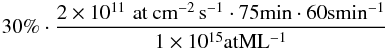 amounting to 0.27 ML in 75 min.
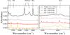 |
Fig. 2 RAIR difference spectra from a co-deposition of H and 16O2 from Cuppen et al. (2010), H2, CO2 and 18O (experiment 1), CO2 and 18O (experiment 2). Spectra are baseline corrected and offset for clarity. The spectra corresponding to experiments 1, 2 and 5 are scaled with a factor 3. Note that the multitude of peaks in the right panel for experiments 1 and 2 are due to water vapor in the setup, and the peaks at 3515 and 3564 cm-1 are also visible in a “pure” CO2 spectrum. |
Experiment 1 does not result in a detectable amount of formed OH or H2O on the basis of their infrared solid-state spectral features. Moreover, there is no significant difference between RAIR spectra of experiments 1 and 2, as demonstrated in Fig. 2. The small features visible in the 1600–1800 cm-1 range are due to water vapor, and they in fact determine the detectable level. Comparing these spectra with a spectrum obtained from a previous co-deposition experiment of H:O2 = 1:1 (Cuppen et al. 2010), where OH, OH·H2O and H2O spectral bands were found at 3548, 3463, 3426, and 1590 cm-1, we conclude that the maximum water production falls below the detection limit of RAIR spectroscopy during a 75 min experiment. Therefore, we performed a 300 min co-deposition (experiment 5 in Table 2). In this case, the water peak at 1590 cm-1 was clearly visible and, moreover, after gently annealing to 110 K at a ramp of 0.5 K min-1 to remove CO2 and O2 from the ice, a RAIR spectrum was recorded where approximately 1 ML of water was visible. The upper limit to water production seen with RAIR spectroscopy thus remains ~0.25 ML for an experiment of 75 min.
3.2.2. QMS
Quadrupole mass spectroscopy allows one to better constrain an upper limit for water formation thanks to its higher sensitivity. Table 2 summarizes the integrated baseline-corrected QMS signals for mass 20 amu (HO). Figure 3 shows the baseline-corrected QMS traces of experiments 1–4 from Table 2, both the co-desorption with CO2 and the thermal desorption of H2O are visible. Experiments 1–3 were performed twice and both traces are shown. The desorption in the region between 14 and 70 K was not taken into further consideration. This is because of the contribution from the species desorbing from the heating tape area in proximity of the substrate, and also because of the oversaturation of the signal by desorption of H2 or D2, as can be concluded from comparing experiments 1 and 3. Experiments 1–3 all were performed twice, and the difference between the sum of the integrated signals of two identical experiments is 16, 5, and 26% respectively, indicating that the overall uncertainty is on the order of 25% or smaller.
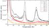 |
Fig. 3 QMS traces of mass 20 amu for experiments 1–4 from Table 2. Spectra are baseline corrected, offset for clarity, and binned by averaging 5 points. Experiments 1–3 have been performed twice, hence two traces are depicted by the solid and dashed lines. |
The upper limit to water production, calculated with Eq. (5), is about a factor 2 lower than concluded from the RAIRS data: 0.14 ML during a 75-min experiment. The m/z = 20 signal of both the co-desorption with CO2 and pure desorption of water was taken into account.
Species that react via the LH mechanism are thermalized and stay on the surface, where they diffuse until they meet. This mechanism can be tested by changing the temperature of the ice. In this case, the production of water is expected to decrease with increasing temperature because of a lower surface abundance of H2 and, moreover, no products should be detected at temperatures above the desorption temperature of one of the reactants. For this reason, the experimental temperatures employed here were 17, 35, and 50 K (experiments 6–8). All detected m/z = 20 signals in these experiments are close to the background level determined at 14 K by experiments 2 and 3. We assume that the observed water is indeed formed – even though this not necessarily has to be the case – and below we discuss various mechanisms. The detected amounts at 17 and 35 K are equal, implying that the LH mechanism probably does not govern any potential reaction, because of the temperature dependence of the residence time at the surface. Moreover, the integrated m/z = 20 signal decreases further when increasing the temperature to 50 K, but it still remains non-negligible.This means that the ER and/or HA mechanisms probably are responsible for any H2O formation, at least in part and most likely even at 14 K. For both mechanisms one or more reaction partners are not thermalized. For the HA mechanism again both reaction partners are present on the surface, but at least one of them is in some excited state (i.e., not thermalized), whereas ER assumes that one reaction partner is present on the surface and the second comes directly from the gas phase and therefore must have a temperature of ~300 K. Both mechanisms in combination with excitation are not expected to be astronomically important because of the longer timescales and the much lower gas-phase temperature in dense molecular clouds. The significance of this reaction pathway in the ISM, therefore, will be negligible.
The reaction itself can proceed either classically activated or through a combination of both a classical and tunneled contribution (e.g., Eq. (4)). Tunneling depends on the mass of the reactants involved. Exchanging hydrogen for deuterium would result in a decrease of the tunneled reaction rate of D2 + O and therefore a decrease in the production of m/z = 22 (DO) compared to m/z = 20 (HO). Comparing the integrated QMS signals of m/z = 22 in experiments 9 and 10 with m/z = 20 in experiment 1 at 125–175 K, we indeed see a large drop up to barely no signal. Therefore, HO formation in experiment 1 through a mechanism in which tunneling plays a role cannot be eliminated. Because of the endothermicity of the reaction, this has to be a combination of classical and tunneling behavior. As explained above, the classical part can be overcome by some excitation effect.
Finally, even in the experiments performed with D2 still HO was detected, which can only be caused by water contamination. From the result found in experiment 9 it is possible to directly estimate the upper limit with ![\begin{eqnarray} [{\rm H}_2^{18}{\rm O}] \left( {(1)} - {(9)} \right) \end{eqnarray}](/articles/aa/full_html/2014/10/aa24252-14/aa24252-14-eq72.png) (6)instead of with Eq. (5). The difference in signal between experiments 1 and 9 was therefore taken as the final range for the upper limit to water production for our KMC model, that is, 0.09 ML in 75 min. Because we wish to determine an upper limit here, we worked with the outcome of experiment 9 and not 10 to guarantee that we remained on the conservative side.
(6)instead of with Eq. (5). The difference in signal between experiments 1 and 9 was therefore taken as the final range for the upper limit to water production for our KMC model, that is, 0.09 ML in 75 min. Because we wish to determine an upper limit here, we worked with the outcome of experiment 9 and not 10 to guarantee that we remained on the conservative side.
4. Theoretical
4.1. Kinetic Monte Carlo model
This section describes the specific kinetic Monte Carlo procedure used for the simulations and focuses on the difference between modeling experimental results and modeling under interstellar relevant conditions. For a more detailed overview of the method we refer to Chang et al. (2005) and Cuppen et al. (2013). The code we used is described in Cuppen & Herbst (2007) and Lamberts et al. (2013, 2014).
The grain is represented by a lattice of 50 × 50 sites with periodic boundary conditions, in which each lattice site can be occupied by one of the following species: H, H2, O, O2, O3, OH, HO2, H2O, and H2O2. Interstitial sites can be only occupied by H, H2, O, and OH. Processes incorporated in the simulations are i) deposition from the gas phase to the surface; ii) desorption from the surface back into the gas phase; iii) diffusion on the surface; iv) reaction, when two species meet each other; and v) (photo)dissociation upon energy addition to the species. Each of these processes is simply modeled as a change in the occupancy of the sites involved. The event rates are assumed to be classically activated and are calculated using (a form of) Eq. (1). The barrier for desorption and diffusion depends on the binding energy of the species to the specific site it occupies. The reaction network consisting of 16 surface reactions and their corresponding rates is taken from Lamberts et al. (2014). Photodissociation is implemented only in the interstellar simulations to investigate the influence of the interstellar radiation field. In this case, the five relevant reactions and their rates are taken from van Dishoeck et al. (2006).
The following strategy was applied: first kinetic Monte Carlo calculations were used to reproduce the experiments with the aim to find an upper limit for the reaction rate (Sect. 4.2). The resulting rate was then used to simulate the formation of interstellar ice on astrochemical timescales with a full water surface reaction network to determine the contribution of the H2 + O reaction to the total production of water ice on interstellar grains in dense clouds (Sect. 4.3). Note that, again, this is a conservative method since we already attributed any possible H2O formation to mechanisms not relevant in the ISM. Below, however, we assume an LH type mechanism. Our reaction network neither includes any species with C or N atoms, which will also consume hydrogen. Here we specifically compare the contributions of the reactions H + O and H2 + O.
4.2. Experimental modeling
All surface abundances increase linearly with time, similar to those for co-deposition experiments in Lamberts et al. (2013, 2014). The final abundances mentioned here were determined after 75 simulated experimental minutes. In all experimental simulations water was produced by the immediate follow-up reaction R2, H + OH → H2O, because of our implementation of zero excess energy for the reaction H2 + O → OH + H. H and OH remain in each other’s vicinity and can thus easily react. The uncertainty in the H2O surface abundance was derived from two different simulations that were each repeated three times. We find values decreasing in time from roughly 25 to 7%, where the largest error bar corresponds to the lowest amount of species on the surface.
The values for the fluxes used in the simulations are equal to those listed in Table 2 for the used experiments. The sticking coefficients were assumed to be unity for the heavier species (18O, 18O2 and CO2), but was set to a conservative value of 0.2 for H2. Experimental results on the sticking of H2 at 300 K to a 10 K surface indeed indicate such low coefficients (Chaabouni et al. 2012). The CO2 flux may be lower because of freeze-out on the cold finger of the cryostat, but, again, to remain on the conservative side, we took the highest value of 1.6 × 10¹⁴. The remaining parameter settings used here are listed in Table 3. In general, the values for the input parameters are subject to some arbitrary choices. Here, all input variables were chosen such that they would result in a high reaction rate of the reaction H2 + O. This is illustrated by the H2 sticking coefficient and the flux of CO2: a low sticking coefficient results in fewer H2 + O encounters and therefore would require a faster reaction rate to produce a result equal to that with a higher coefficient. The same holds for a decrease of the CO2 flux.
Lowest, highest and standard parameters used and varied in the experimental simulations.
Summary of the impact of each parameter on the O3 and H2O abundances in the ice.
The approach taken here is to find a set of parameters that allows reproducing the experimental upper limit of 0.09 ML (see Sect. 3.2) in 75 min of experiment. To do this, we varied several parameters, as mentioned in Table 3. First, the diffusion barrier of H2 was set to 195, 220 and 250 K. Next, we performed simulations using barriers for oxygen atom diffusion with 330, 555, and 1100 K. The latter value has been used in earlier studies (Lamberts et al. 2013, 2014) and the second value is half of this number. Very recently, literature values have become available (e.g., Lee & Meuwly 2014; Congiu et al. 2014) that predict values between 350 and 1000 K, the domain embedded by our chosen barrier values. The reaction rates of the reactions O2 + O and H2 + O were also varied. The first reaction rate was set to the value used in a previous study (Lamberts et al. 2013, 8.2 × 10⁻⁵ s-1) and to a value corresponding to a barrierless reaction (1.0 × 10¹² s-1). The second rate was set to 1.35 × 10⁻¹, 5.5, 5.1 × 101, 2.2 × 10², and 9.8 × 10² s-1. These values represent exactly the range in which the reaction H2 + O becomes effective in competing with diffusion and other reactions. In other words, for reaction rates below 1.35 × 10⁻¹ s-1 the reaction does not occur at all. This sensitive window of reaction rates was found by performing several test simulations used to probe the influence of the parameters. We started with two models for each parameter, using the lowest and highest value while keeping all other parameters constant to their standard value, as indicated in the final row of Table 3. Because of the dominant role of kH2 + O, the influence of any other parameter was typically checked at two different reaction rates. Only when a dependence on a particular parameter was found, we varied that specific parameter in additional simulations while keeping other parameters constant to their standard value. Therefore, we did not use a full grid of models, but performed a total of 15 simulations. The resulting O3 and H2O abundances are summarized in Table 4.
The diffusion rates of both O and H2 only play a role when the reaction with the O atom is almost prohibited. In this case, a high diffusion rate leads to a lower water production because of the favorable competition with respect to reaction. The amount of O3 produced in the simulations does not depend on the diffusion rate of oxygen atoms, but shows a strong dependence on the reaction rate of O2 + O. We previously used a reaction rate of 8.2 × 10⁻⁵ s-1 (Lamberts et al. 2013). Here we see that a faster rate is needed to reproduce the amounts detected by RAIR spectroscopy. We return to this in the next section.
From Table 4 it can be deduced that for the production of water the reaction rate itself has the strongest impact on the final abundances, that is, kH2 + O. For most simulations the final H2O abundance remains below the experimental upper limit of 0.09 ML. In Fig. 4, the surface abundances of O, O2, O3, H2 and H2O are depicted over a simulated period of 37.5 min for simulation 3 in Table 4, which we define as the upper-limit simulation. This was a co-deposition experiment and simulation, therefore the profile of surface abundances is increasing linearly with time. The high amount of H2 should be interpreted as 1.1 ML distributed over the total ice thickness of 360 ML. The total ice thickness is mainly determined by the high CO2 flux, and therefore a deposited H2 molecule either reacts, desorbs, or is covered by another CO2 molecule. This means that on average there is 0.003 ML of H2 in each monolayer, and thus this corresponds to the average surface coverage at any given time. The final H2O abundance in this figure is 0.045 ML because of the reduced time scale. The value of kexp.max(13.5 K) = 2.2 × 10² s-1 leads to this H2O production, which corresponds to the experimentally determined value. This rate was be used to simulate water formation in the ISM through H2 + O.
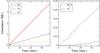 |
Fig. 4 Surface abundances of O, O2, O3, H2, and H2O in time for the upper-limit simulation. One should realize that the total amount of deposited ice over the course of this simulation is 360 ML. The dominant component, by far, is CO2 (not shown) because of its high flux. |
4.3. Astrochemical modeling
Two dense clouds with different temperature, density, and UV field were studied. Their physical parameters were chosen to be identical to those of dense clouds I and II in Lamberts et al. (2014), as summarized in Table 5. The high densities nH and simultaneous low temperatures, but high AV values mimic typical values found in dense clouds. A major difference between the present and previous work is the inclusion of endothermicity of reaction R1. In the preceding study, we included an excess energy of 1400 K for each reaction in the water formation network with two reaction products, and the energy was spread over these products. The excess energy for the endothermic reaction H2 + O was therefore explicitly set to 0 K, all other two-product reactions obtain a reaction heat of 1400 K. We used the same full water reaction network, but following the outcome of Lamberts et al. (2013, 2014), we omitted the reaction channel H + HO2→ H2O2. The network consisted of 16 reactions.
The main parameter varied in the astrochemical simulations is the rate of reaction R1, ranging between the fastest kexo.tunn. and the slowest kendo.tunn., as explained in Sect. 2. From the experiments we deduced in Sect. 3.2 that if water is produced starting from H2 + O, it can only be by a mechanism that overcomes the endothermicity classically followed by tunneling through the barrier, as indicated in Fig. 1 and Eq. (4). We scale the reaction rate determined experimentally at 13.5 K to rates relevant at 10 and 12 K – the surface temperatures of the grains in the dense cloud studied here – with the approach outlined below:  (7)Here, we assumed that the endothermicity of the reaction, ΔE, is well constrained by the gas-phase value of 960 K. The tunneling mechanism, activation energy, and pre-exponential factor were not specifically considered (compare to Eq. (4)), but were all combined in the factor C, which was considered temperature independent over the small temperature range studied here.
Contributions of the different surface reaction routes to OH and H2O formation after a coverage of 1 ML is reached, and the total produced water rate for dense clouds I and II for different values of kH2 + O.
Table 6 gives the contributions of the different surface reaction routes to OH and H2O formation and the total amount of H2O produced per kyr in the simulations. Three different reaction rates were considered: i) assuming exothermic tunneling with Eq. (2); ii) using the experimentally determined highest rate with Eq. (7); and iii) assuming that Ea + ΔE = 3000 K in Eq. (4). The results presented here were obtained at a time of ~2.0 × 10⁴ and ~3.5 × 10³ years for the two clouds. This may seem too short to be relevant on an interstellar scale, and is due to the high computational costs, but all abundances increase linearly or reach a steady-state abundance before this time. Moreover, all values were calculated after the grain was already covered with a total of 1 ML of species.
The following reaction channels are considered in Table 6: first, the production of the OH radical was broken down into the separate contributions of five reaction routes, namely H2 + O, H + O, H + HO2, H + O3, and H + H2O2. For cloud I, changing the reaction rate of R1 simply shifts the main production route from H2 + O to H + O for decreasing rates. For cloud II, however, there is more oxygen than atomic H present in the cloud. Allowing the reaction H2 + O to proceed thus leads to a much higher OH production.
Water can also be formed by multiple reaction routes, but the important two here are H + OH and H2 + OH. For lower densities, the total water production rate does not change substantially between the three rates. At higher densities, the larger abundance of OH translates immediately into more produced H2O, since the products of reaction R1, that is, H and OH, remain again in each other’s vicinity.
Furthermore, Table 6 clarifies for the upper limit to the reaction rate, kexp.max., that the reaction H2 + O only contributes at most 11% to the formation of OH on the surface of dust grains in cloud I and does not contribute at all in cloud II. Since we chose all parameters conservatively, this is an absolute upper limit. Higher H2 sticking probabilities, lower CO2 flux due to freeze-out on the cold finger or nonthermalized effects as detailed in Sects. 3.2 and 4.2 all lead to lower rates.
The effect of the O diffusion barrier was investigated by simulating with the values 555 and 1100 K. Although the total water production does not change much, the relative contributions of the reactions that produce OH radicals do: with a faster O diffusion, the competition between diffusion and the reaction H2 + O favors diffusion, leaving O free on the surface to react with other species. Consequently, the reactions H + O, O + O or O + O2 play a larger role, the extent of which depends on the density. Furthermore, increasing the reaction rate for O3 formation results in a larger contribution of the reaction channel H + O3. In the end, these effects will also decrease the efficiency of the reaction H2 + O.
5. Astrophysical implications
Since the reaction H2 + O only contributes to at most 11% to the formation of OH, water formation is dominated by the other reaction routes, such as O + H, O2 + H, OH + H and OH + H2. This implies that depending on the ratio of O/H in the gas phase, the limiting factor to the water formation rate in dark clouds is the amount of H atoms available. Additionally, for high O/H ratios, a higher diffusion rate of O atoms can lead to more reactions of the type O + O (Congiu et al. 2014). This does not mean that water formation is prohibited, since the reaction channel O2 + H can also lead to efficient water formation (Ioppolo et al. 2010; Cuppen et al. 2010; Lamberts et al. 2013).
The experimentally found upper limit for the reaction rate, Eq. (7), can be compared with the values of the reaction rates where exothermic tunneling was assumed. The final two entries of Table 1 show that these rates (at 10 K) are always higher. Therefore, the assumed importance of the reaction H2 + O for the deuterium fractionation ratios of water on the surfaces of dust grains has to be considered with care (Cazaux et al. 2010, 2011). Their HDO/H2O ratio found at low temperatures results from the assumption that the reaction HD + O proceeds via tunneling and therefore mainly produces OH + D. There might be much more HDO formed on the surface of dust, depending on the main water formation route in the specific region in the interstellar medium (through atomic or molecular oxygen).
6. Conclusions
We studied experimentally and by modeling the significance of the reaction H2 + O → H + OH in the framework of the solid-state water formation network in interstellar ice (analogs).
From precisely executed temperature-programmed desorption experiments in an UHV setup that brought together H2 and O in a matrix of CO2, we established an experimental upper limit of the water production. If this amount of water is indeed produced on the surface instead of coming from an additional source of contamination, this can only be caused by a combined classical and tunneled reaction mechanism, based on Eq. (4). An upper limit for the reaction rate was found using a microscopic kinetic Monte Carlo model that converts the maximum number of molecules formed into a possible reaction rate: 1.68 × 1033·exp(−960/T) s-1. By incorporating this rate into simulations ran under astrochemically relevant parameters, we found that the reaction H2 + O does not contribute more than 11% to the formation of water in dense clouds in the interstellar medium.
This number is an absolute upper limit, because all numbers used are conservative estimates. It is likely that in space the efficiency is substantially lower.
Acknowledgments
H.M.C. is grateful for support from the VIDI research program 700.10.427, which is financed by The Netherlands Organization for Scientific Research (NWO) and from the European Research Council (ERC-2010-StG, Grant Agreement no. 259510-KISMOL). T.L. is supported by the Dutch Astrochemistry Network financed by The Netherlands Organization for Scientific Research (NWO). Support for S.I. from the Niels Stensen Fellowship and the Marie Curie Fellowship (FP7-PEOPLE-2011-IOF-300957) is gratefully acknowledged. The SLA group has received funding from the European Community’s Seventh Framework Programme (FP7/2007- 2013) under grant agreement n.238258, the Netherlands Research School for Astronomy (NOVA) and from the Netherlands Organization for Scientific Research (NWO) through a VICI grant.
References
- Andersson, S., Goumans, T. P. M., & Arnaldsson, A. 2011, Chem. Phys. Lett., 513, 31 [NASA ADS] [CrossRef] [Google Scholar]
- Anton, R., Wiegner, T., Naumann, W., et al. 2000, Rev. Sci. Instrum., 71, 1177 [NASA ADS] [CrossRef] [Google Scholar]
- Arnaut, L. G., Formosinho, S. J., & Barroso, M. 2006, J. Mol. Struct., 786, 207 [NASA ADS] [CrossRef] [Google Scholar]
- Baulch, D. L., Cobos, C. J., Cox, R. A., et al. 1992, J. Phys. Chem. Ref. Data, 21, 411 [NASA ADS] [CrossRef] [Google Scholar]
- Bell, R. P. 1980, The tunnel effect in chemistry (London: Chapman and Hall) [Google Scholar]
- Bergin, E. A., & Tafalla, M. 2007, Annu. Rev. Astron. Astrophys., 45, 339 [Google Scholar]
- Cazaux, S., Cobut, V., Marseille, M., Spaans, M., & Caselli, P. 2010, A&A, 522, A74 [NASA ADS] [CrossRef] [EDP Sciences] [Google Scholar]
- Cazaux, S., Caselli, P., & Spaans, M. 2011, ApJ, 741, L34 [NASA ADS] [CrossRef] [Google Scholar]
- Chaabouni, H., Bergeron, H., Baouche, S., et al. 2012, A&A, 538, A128 [NASA ADS] [CrossRef] [EDP Sciences] [Google Scholar]
- Chang, Q., Cuppen, H. M., & Herbst, E. 2005, A&A, 434, 599 [NASA ADS] [CrossRef] [EDP Sciences] [Google Scholar]
- Congiu, E., Minissale, M., Baouche, S., et al. 2014, Faraday Disc., 168 [Google Scholar]
- Cuppen, H. M., & Herbst, E. 2007, ApJ, 668, 294 [Google Scholar]
- Cuppen, H. M., Ioppolo, S., Romanzin, C., & Linnartz, H. 2010, Phys. Chem. Chem. Phys., 12, 12077 [NASA ADS] [CrossRef] [Google Scholar]
- Cuppen, H. M., Karssemeijer, L. J., & Lamberts, T. 2013, Chem. Rev., 113, 8840 [CrossRef] [Google Scholar]
- Dulieu, F., Amiaud, L., Congiu, E., et al. 2010, A&A, 512, A30 [NASA ADS] [CrossRef] [EDP Sciences] [Google Scholar]
- Garrod, R. T., & Herbst, E. 2006, A&A, 457, 927 [NASA ADS] [CrossRef] [EDP Sciences] [Google Scholar]
- Hiraoka, K., Miyagoshi, T., Takayama, T., Yamamoto, K., & Kihara, Y. 1998, ApJ, 498, 710 [NASA ADS] [CrossRef] [Google Scholar]
- Ioppolo, S., Cuppen, H. M., Romanzin, C., van Dishoeck, E. F., & Linnartz, H. 2008, ApJ, 686, 1474 [NASA ADS] [CrossRef] [Google Scholar]
- Ioppolo, S., Cuppen, H. M., Romanzin, C., van Dishoeck, E. F., & Linnartz, H. 2010, Phys. Chem. Chem. Phys., 12, 12065 [NASA ADS] [CrossRef] [Google Scholar]
- Ioppolo, I., Fedoseev, G., Lamberts, T., Romanzin, C., & Linnartz, H. 2013, Rev. Sci. Instrum., 84, 073112 [NASA ADS] [CrossRef] [Google Scholar]
- Lamberts, T., Cuppen, H. M., Ioppolo, I., & Linnartz, H. 2013, Phys. Chem. Chem. Phys., 15, 8287 [CrossRef] [Google Scholar]
- Lamberts, T., de Vries, X., & Cuppen, H. M. 2014, Faraday Disc., 168, 327 [NASA ADS] [CrossRef] [Google Scholar]
- Lee, M. W., & Meuwly, M. 2014, Faraday Disc., 168 [Google Scholar]
- Miyauchi, N., Hidaka, H., Chigai, T., et al. 2008, Chem. Phys. Lett., 456, 27 [NASA ADS] [CrossRef] [Google Scholar]
- Mokrane, H., Chaabouni, H., Accolla, M., et al. 2009, ApJ, 705, L195 [NASA ADS] [CrossRef] [Google Scholar]
- Oba, Y., Miyauchi, N., Hidaka, H., et al. 2009, ApJ, 701, 464 [NASA ADS] [CrossRef] [Google Scholar]
- Oba, Y., Watanabe, N., Hama, T., et al. 2012, ApJ, 749, 67 [NASA ADS] [CrossRef] [Google Scholar]
- Oba, Y., Osaka, K., Watanabe, N., Chigai, T., & Kouchi, A. 2014, Faraday Disc., 168, 185 [NASA ADS] [CrossRef] [Google Scholar]
- Rogers, S., Wang, D., Kuppermann, A., & Walch, S. 2000, J. Phys. Chem. A, 104, 2308 [CrossRef] [Google Scholar]
- Romanzin, C., Ioppolo, S., Cuppen, H. M., van Dishoeck, E. F., & Linnartz, H. 2011, J. Chem. Phys., 134, 084504 [NASA ADS] [CrossRef] [Google Scholar]
- Taquet, V., Peters, P. S., Kahane, C., et al. 2013, A&A, 550, A127 [NASA ADS] [CrossRef] [EDP Sciences] [Google Scholar]
- van Dishoeck, E. F., Jonkheid, B., & van Hemert, M. C. 2006, Faraday Disc., 133, 231 [Google Scholar]
All Tables
Calculated reaction rates for the reaction H2 + O assuming classical and tunneled contributions.
List of (control) experiments and integrated baseline-corrected QMS signals for m/z = 20 and 22, i.e. HO and DO, and the calculated HO abundance in ML.
Lowest, highest and standard parameters used and varied in the experimental simulations.
Contributions of the different surface reaction routes to OH and H2O formation after a coverage of 1 ML is reached, and the total produced water rate for dense clouds I and II for different values of kH2 + O.
All Figures
|
Fig. 1 Schematic representation of the energy level diagram of an exothermic and endothermic reaction. |
| In the text | |
|
Fig. 2 RAIR difference spectra from a co-deposition of H and 16O2 from Cuppen et al. (2010), H2, CO2 and 18O (experiment 1), CO2 and 18O (experiment 2). Spectra are baseline corrected and offset for clarity. The spectra corresponding to experiments 1, 2 and 5 are scaled with a factor 3. Note that the multitude of peaks in the right panel for experiments 1 and 2 are due to water vapor in the setup, and the peaks at 3515 and 3564 cm-1 are also visible in a “pure” CO2 spectrum. |
| In the text | |
|
Fig. 3 QMS traces of mass 20 amu for experiments 1–4 from Table 2. Spectra are baseline corrected, offset for clarity, and binned by averaging 5 points. Experiments 1–3 have been performed twice, hence two traces are depicted by the solid and dashed lines. |
| In the text | |
|
Fig. 4 Surface abundances of O, O2, O3, H2, and H2O in time for the upper-limit simulation. One should realize that the total amount of deposited ice over the course of this simulation is 360 ML. The dominant component, by far, is CO2 (not shown) because of its high flux. |
| In the text | |
Current usage metrics show cumulative count of Article Views (full-text article views including HTML views, PDF and ePub downloads, according to the available data) and Abstracts Views on Vision4Press platform.
Data correspond to usage on the plateform after 2015. The current usage metrics is available 48-96 hours after online publication and is updated daily on week days.
Initial download of the metrics may take a while.