| Issue |
A&A
Volume 570, October 2014
|
|
|---|---|---|
| Article Number | A28 | |
| Number of page(s) | 21 | |
| Section | Extragalactic astronomy | |
| DOI | https://doi.org/10.1051/0004-6361/201424116 | |
| Published online | 10 October 2014 | |
Molecular line emission in NGC 1068 imaged with ALMA
II. The chemistry of the dense molecular gas⋆
1 Department of Physics and Astronomy, UCL, Gower St., London, WC1E 6BT, UK
e-mail: This email address is being protected from spambots. You need JavaScript enabled to view it.
2 Observatorio Astronomico Nacional (OAN) – Observatorio de Madrid, Alfonso XII, 3, 2814 Madrid, Spain
3 INAF – Osservatorio Astrofisico di Arcetri, Largo E. Fermi 5, 50125 Firenze, Italy
4 Max-Planck-Institut für Radioastronomie, Auf dem Hg¨el 69, 53121 Bonn, Germany
5 Astronomy Department, King Abdulaziz University, PO Box 80203, 21589 Jeddah, Saudi Arabia
6 I. Physikalisches Institut, Universität zu Köln, Zülpicher Str. 77, 50937 Köln, Germany
7 Institut de Radio Astronomie Millimétrique (IRAM), 300 rue de la Piscine, Domaine Universitaire de Grenoble, 38406 St. Martin d’ Hères, France
8 Kapteyn Astronomical Institute, University of Groningen, PO Box 800, 9700 AV Groningen, The Netherlands
9 Department of Radio and Space Science with Onsala Observatory, Chalmers University of Technology, 439 94 Onsala, Sweden
10 Observatoire de Paris, LERMA, 61 Av. de l’Observatoire, 75014 Paris, France
11 Max-Planck-Institut für Astronomie, Königstuhl, 17, 69117 Heidelberg, Germany
12 INAF – Istituto di Radioastronomia & Italian ALMA Regional Centre, via Gobetti 101, 40129 Bologna, Italy
13 Instituto de Astrofísica de Andalucía (CSIC), Glorieta de la Astronomía s/n Granada, Granada 18080, Spain
14 Leiden Observatory, Leiden University, PO Box 9513, 2300 RA Leiden, The Netherland
15 Department of Physics and Astronomy, Rutgers, The State University of New Jersey, Piscataway, NJ 08854, USA
16 Université de Toulouse, UPS-OMP, IRAP, 31028 Toulouse, France
17 Max-Planck-Institut für extraterrestrische Physik, Postfach 1312, 85741 Garching, Germany
Received: 2 May 2014
Accepted: 12 July 2014
Abstract
Aims. We present a detailed analysis of Atacama Large Millimeter/submillimeter Array (ALMA) Bands 7 and 9 data of CO, HCO+, HCN, and CS, augmented with Plateau de Bure Interferometer (PdBI) data of the ~200 pc circumnuclear disc (CND) and the ~1.3 kpc starburst ring (SB ring) of NGC 1068, a nearby (D = 14 Mpc) Seyfert 2 barred galaxy. We aim to determine the physical characteristics of the dense gas present in the CND, and to establish whether the different line intensity ratios we find within the CND, as well as between the CND and the SB ring, are due to excitation effects (gas density and temperature differences) or to a different chemistry.
Methods. We estimate the column densities of each species in local thermodynamic equilibrium (LTE). We then compute large one-dimensional, non-LTE radiative transfer grids (using RADEX) by using only the CO transitions first, and then all the available molecules to constrain the densities, temperatures, and column densities within the CND. We finally present a preliminary set of chemical models to determine the origin of the gas.
Results. We find that, in general, the gas in the CND is very dense (>105 cm-3) and hot (T> 150 K), with differences especially in the temperature across the CND. The AGN position has the lowest CO/HCO+, CO/HCN, and CO/CS column density ratios. The RADEX analyses seem to indicate that there is chemical differentiation across the CND. We also find differences between the chemistry of the SB ring and some regions of the CND; the SB ring is also much colder and less dense than the CND. Chemical modelling does not succeed in reproducing all the molecular ratios with one model per region, suggesting the presence of multi-gas phase components.
Conclusions. The LTE, RADEX, and chemical analyses all indicate that more than one gas-phase component is necessary to uniquely fit all the available molecular ratios within the CND. A higher number of molecular transitions at the ALMA resolution is necessary to determine quantitatively the physical and chemical characteristics of these components.
Key words: galaxies: active / galaxies: individual: NGC 1068 / galaxies: ISM / galaxies: nuclei / molecular processes / radio lines: galaxies
Tables 5–11 are available in electronic form at http://www.aanda.org
© ESO, 2014
1. Introduction
Galaxy evolution is now thought to depend on feedback mechanisms whereby star formation is inhibited at some point in the galaxy’s lifetime either by an active galactic nucleus (AGN) or by stellar feedback through winds and supernovae. Up to now it has been very difficult to capture the observational signatures of mechanical feedback directly, but recent molecular emission-line observations are opening a new window on this aspect of galaxy evolution by the detection of molecular outflows (e.g. Aalto et al. 2012; Feruglio et al. 2010; Veilleux et al. 2013; Combes et al. 2013; Cicone et al. 2014; García-Burillo et al. 2014, hereafter Paper I). Signs of radiative feedback in galactic nuclei are complicated by the interplay of a central starburst with an AGN. Most of the gas in galaxy centres resides in molecules, and because most galaxy centres tend to be obscured by dust, it is crucial to identify the chemical nature of the gas involved and to determine the physical conditions that are most prone to lead to a starburst; hence, submillimeter molecular tracers have become one of the most important probes of physical conditions in galaxy nuclei. Through comparison with models, molecular abundances, and line ratios can be used to infer physical conditions, but also to constrain the chemical reactions that drive molecule formation and destruction in irradiated regions. Molecular abundances in starburst and AGN-dominated galaxies are usually interpreted through models for photon-dominated regions (PDRs) and X-ray dominated regions (XDRs), and are among the best diagnostics for disentangling massive star formation and the influence of an AGN (Meijerink et al. 2007; Bayet et al. 2009). More recently, in an attempt to interpret the observations of molecules that may arise from very dense and possibly shocked gas, chemical gas-grain models as well as shocks models have also been used to interpret molecular lines in these galaxies (e.g. Aladro et al. 2013).
Massive stars usually form in huge concentrations of dense (n(H2) ~ 105 cm-3) and warm (Tk ≥ 50 K) molecular gas, which are able to survive disruptive forces (winds or radiation) from nearby newly formed stars longer than the gas in the local interstellar medium (ISM; e.g. Zinnecker & Yorke 2007). Molecules constitute a significant fraction of the interstellar gas and, because of their high critical densities, trace the dense regions where star formation takes place (e.g. Omont 2007). Moreover, in general and at large scales, the overall abundance of molecules is determined by the density of the gas, which favours their formation, and the energetic processes, such as UV or X-ray radiation, which in general tend to destroy molecules. Subject to a proper interpretation, observations of molecules can be used to (i) trace the matter that is the reservoir or leftover of the star formation process; (ii) trace the process of star formation itself; and (iii) determine the influence of newly-formed stars or an AGN on their environments and hence the galaxy energetics.
Although 12CO is the most common tracer of the global molecular reservoir, for the nearest sources we now have an inventory of species that allow us to study in detail the different gas components within a galaxy as well as its energetics (e.g. García-Burillo et al. 2002; Wang 2004; Usero et al. 2004; Fuente et al. 2008; Aalto et al. 2011; Martín et al. 2011; Aladro et al. 2013; Costagliola et al. 2011; Kamenetzky et al. 2011; Watanabe et al. 2014). A common trend observed in recent surveys is a chemical diversity and complexity that is hard to explain with a one-component gas phase. As with our own Galaxy, it is becoming clear that different molecules will trace different regions of a galaxy (e.g. Meier & Turner 2005, 2012; Usero et al. 2006; García-Burillo et al. 2010) from the cold, relatively low density molecular gas traced by CO, to highly shocked regions, traced by e.g. SiO, and finally to very high density star forming clouds (traced by e.g. CS and possibly CH3OH). Often high abundances of particular species such as HCO+ are automatically attributed to the presence of strong PDRs, since this molecule is indeed abundant in the presence of a strong UV field, regardless of the metallicity, cosmic ray ionization rate or density of the galaxy (Bayet et al. 2009). Nevertheless, this species is also highly enhanced when the cosmic ray or X-ray ionization rates are high, regardless of the UV field (Bayet et al. 2011; Meijerink & Spaans 2005). This apparent degeneracy is common to most molecules and again reflects the fact that chemistry is a non-linear process influenced by a combination of energetics and physical conditions.
Galaxies characterized by both AGN and vigorous circumnuclear star formation present a complex combination of energetic processes, including UV-rays and X-rays plus shocks associated with AGN feedback, which can take over the processing of ISM in the circumnuclear regions (e.g. Combes 2006). For these objects, the connection between the starburst and the central AGN is still unknown, although large amounts of dense circumnuclear gas imply that the two regions must interact. There is no unique molecular tracer for such dense gas in these complex systems; theoretical models (e.g. Bayet et al. 2008, 2009) show that all the molecules that ought to be detectable in AGN plus starburst systems are also characteristics of “pure” starburst galaxies. High-resolution imaging of molecular line emission is a key to disentangling the contribution of the starburst from that of the AGN component in composite systems. Observations seem to indicate that abundance ratios of HCN/HCO+ may help trace the dominating energetic processes (e.g. Krips et al. 2008, 2011; Aalto et al. 2011; Loenen et al. 2008); however, the chemistry of both these species is highly dependent on the physical conditions of the gas as well as on its energetics. Galaxies where starbursts and AGN are both present therefore require both high spatial resolution and targeted multi-species, multi-line observations to disentangle and characterize the energetics and chemical effects of the molecular gas.
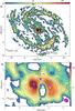 |
Fig. 1 CO (3–2) velocity-integrated intensity map, measured in Jy/beam km s-1 over a 460 km s-1 window, obtained with ALMA (see Paper I Fig. 4 for more details). The central position is the phase tracking center (J2000( RA◦, Dec◦) = (02h42m40 |
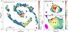 |
Fig. 2 Left: velocity-integrated intensity ratios CO(3–2)/CO(1–0) in the CND as well as in the SB ring. Right: CO(6–5)/CO(3–2) and CO(2–1)/CO(1–0) in the CND. The filled ellipses represent the spatial resolutions used to derive the line ratio maps: 2′′ × 1.1′′PA = 22° for CO(3–2)/CO(1–0) and CO(2–1)/CO(1–0); 0.6′′ × 0.5′′PA = 60° for CO(6–5)/CO(3–2). |
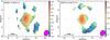 |
Fig. 3 Velocity-integrated intensity ratios HCN(4–3)/HCN(1–0) (left) and HCO+(4–3)/HCO+(1–0) (right) across the CND as well as in the SB ring. The filled ellipses in the lower right corners represent the spatial resolutions used to derive the line ratio maps: 6.6′′ × 5.1′′ PA = 157°, for both panels. |
One of the most studied examples of a composite starburst/AGN galaxy is NGC 1068, a prototypical nearby (D ~ 14 Mpc) Seyfert 2 galaxy, which is the subject of numerous observational campaigns focussed on the study of the fuelling of its central region and related feedback activity using molecular line observations (e.g. Usero et al. 2004; Israel 2009; Kamenetzky et al. 2011; Hailey-Dunsheath et al. 2012; Aladro et al. 2013). Interferometric observations of CO, as well as HCN, HCO+, CS, and SiO (e.g. Tacconi et al. 1994; Schinnerer et al. 2000; García-Burillo et al. 2010; Krips et al. 2011; Tsai et al. 2012) clearly show that molecular tracers of dense gas are essential to spatially resolve the distribution, kinematics, and excitation of the circumnuclear gas of NGC 1068 and to study the relationship between the r ~ 1 − 1.5 kpc starburst (SB) ring and the r ~ 200 pc circumnuclear disc (CND) located around the AGN. A summary of interferometric observations of NGC 1068 can be found in the accompanying Paper I, and references therein. We summarize below the main results of Paper I and the aims of the present work.
In order to probe the bulk of the dense molecular gas in the r ~ 2 kpc disc of NGC 1068, we carried out Atacama Large Millimeter/submillimeter Array (ALMA) Cycle 0 observations in Bands 7 and 9 of several molecular transitions, namely CO (3–2) and (6–5), HCO+ (4–3), HCN (4–3), and CS (7–6) within the r ~ 200 pc CND as well as in the ~1–1.5 kpc SB ring. The data and their reduction are detailed in Paper I. We list below the main observational results of Paper I that are relevant to this work:
-
We found evidence from several tracers thatthe kinematics of the dense molecular gas(n(H2) > 105 cm-3) from r ~ 50 pc out to r ~ 400 pc are shaped by a massive (Mgas ~ 2.7 × 10⁷M⊙) outflow, which reveals the signature of mechanical feedback produced by the AGN. The outflow involves a sizeable fraction (≥50%) of the total gas reservoir in this region.
-
Molecular line ratios derived from the ALMA data show significant differences between the SB ring and the CND. Furthermore, line ratio maps at the 20–35 pc resolution of ALMA show up to order-of-magnitude changes inside the CND. Changes are correlated with the UV/X-ray illumination of the molecular gas at the CND by the AGN. Overall, these results hint at a strong AGN radiative feedback on the excitation/chemistry of the molecular gas.
In the present paper, we concentrate on the chemical analysis of the gas within the CND and towards a particularly prominent star-forming knot of the SB ring, with the aim of quantifying the chemical differentiation and of determining the chemical origin of such differentiation. This is the highest resolution multi-line/multi-species chemical study of this object to date, and allows us, for the first time, to spatially resolve and study sub-regions within the CND.
This paper is sub-divided as follows: in Sect. 2 we report the molecular line ratios and briefly describe the sub-regions of the CND, as determined by our ALMA observations in Paper I; in Sect. 3 we analyse the data by performing local thermodynamical equilibrium (LTE) calculations, as well as radiative transfer modelling with RADEX, developed by Van der Tak et al. (2007). In Sect. 4, we attempt to interpret the data via chemical modelling; in Sect. 5, we list our conclusions.
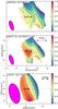 |
Fig. 4 Zoomed in velocity-integrated intensity ratios HCN(4–3)/HCN(1–0), HCO+(4–3)/HCO+(1–0) and CS(7–6)/CS(2–1) in the CND. The filled ellipses represent the spatial resolutions used to derive the line ratio maps: 2′′ × 0.8′′, PA = 19° for HCN(4–3)/HCN(1–0) and HCO+(4–3)/HCO+(1–0); 6.6′′ × 3.2′′ PA = 16° for CS(7–6)/CS(2–1). |
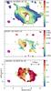 |
Fig. 5 HCN(4–3)/CO(3–2), CS(7–6)/CO(3–2) and HCN(4–3)/ HCO+(4–3) velocity-integrated intensity ratios in the CND. The filled ellipses represent the spatial resolutions used to derive the line ratio maps: 0.6′′ × 0.5′′ PA = 60°, for all panels. |
2. Molecular line ratios
2.1. Methodology
Figure 1 shows the velocity-integrated intensity map of CO(3–2) in the disc of NGC 1068 obtained with ALMA. This is a reproduction of Fig. 4 from Paper I and can be used as a reference “chart” for the present paper. In Figs. 2 to 6, we present the molecular line ratios of the velocity-integrated intensities, in Tmb × Δv units (K km s-1), used for our study of the CND and the SB ring. Prior to deriving the line ratios, all the maps have been referred to the same tracking centre first and then degraded to the lower/common spatial resolution of the data used to derive each line ratio. The degrading is performed in the plane of the sky by an adequate Gaussian convolution kernel specifically adapted for each line ratio.
We show, and subsequently in our analysis use, line ratios which can be considered independent, given the limited number of different intensities available for each region. To that purpose, we combined the ALMA maps presented in Paper I with a set of interferometric images of NGC 1068 obtained by the IRAM Plateau de Bure Interferometer (PdBI) for the lower-J transitions of the same molecular species observed by ALMA, but with spatial resolutions that are comparatively lower in the PdBI maps. In particular, some of the ratios make use of the PdBI data for CO(1–0) and CO(2–1) (taken from Schinnerer et al. 2000), HCO+(1–0) and HCN(1–0) (taken from García-Burillo et al. 2008; Usero et al., in prep.), and CS(2–1) transitions (taken from Tacconi et al. 1997).
The adopted methodology for all the analyses, except for that in Sect. 3.2.3, required that all interferometric images, obtained with original spatial resolutions that range from 20 to 350 pc for the CND (see Table 1 for details), and from 100 pc (for the CO(3–2)/CO(1–0) ratio) to 400 pc (for the rest) for the SB ring, first had to be degraded down to the lower/common spatial resolution of the two transitions involved in each case. For the SB ring, the downgrade to 400 pc in spatial resolution is required in order to recover the emission from the SB ring of the HCN (1–0) and HCO+ (1–0) PdBI data. Intensities were calculated by integrating inside a common 460 km s-1 velocity window (–230, 230 km s-1 relative to the systemic velocity). We also used a common 3σ clipping threshold on the intensities when we derived the ratios to enhance the reliability of the images. For the sake of simplicity, the figures are all centred around the same nominal position of the phase tracking centre adopted in Paper I (J2000( RA◦, Dec◦) = (02h42m40 771), (–00°00′47
 84)).
84)).
None of the maps used to derive the line ratios include short-spacing correction, however, we estimate that the amount of flux filtered in the interferometric images used in this work starts to be significant only at scales >6″. This is well above the lowest spatial resolution of any of the line ratio maps used in this work, where we purposely use fluxes extracted from single apertures that range from ~0.5″ to ~5″ to minimize the bias due to the lack of short spacings.
In our analysis of line ratios, we also use single-dish (IRAM 30 m) estimates of the 12C/13C isotopic line ratios for CO, HCN, and HCO+ to constrain the opacity range of the solutions (Papadopoulos & Seaquist 1999; Usero et al. 2004; Usero, priv. comm.).
2.2. The ALMA “topology” of NGC 1068
From Figs. 2 to 6 and also summarizing the findings from Paper I, we find that overall molecular line ratios show significant differences between the SB ring and the CND. In particular, ratios that measure the excitation of CO, HCN, and HCO+ (like the 3–2/1–0 ratio of CO or the 4–3/1–0 ratio of HCN or HCO+) are a factor of 2–5 higher in the CND on average. Furthermore, mixed ratios that involve transitions of different species having distinctly different critical densities, (for example, HCN(1–0)/CO(1–0) or HCN(1–0)/HCO+(1–0)), are also a factor 2–5 higher in the CND relative to the SB ring. Taken at face value, this result hints at a comparatively higher excitation and/or enhanced abundances of dense gas tracers in the CND. Disentangling excitation from chemistry effects is crucial if we are to interpret the observed differences between the SB and the CND, and it is one of the aims of this paper.
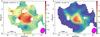 |
Fig. 6 HCN(1–0)/HCO+(1–0) velocity-integrated intensity ratio (left) and the HCN(1–0)/CO(1–0) velocity-integrated intensity ratio (right) in the SB ring. The filled ellipses represent the spatial resolutions used to derive the line ratio maps: 6.6′′ × 5.1′′ PA = 157°. |
Original spatial resolution in parsecs for all (ALMA as well as PdBI) molecular transitions used in this paper.
As discussed in Paper I, molecular line ratios at the full resolution of our ALMA data (~0.3′′–0.5′′, or 20–35 pc at the assumed distance of 14 Mpc) allow us to measure significant differences within the CND. In the following, we define five spatially resolved sub-regions inside the CND, denoted as E Knot, W Knot, AGN, CND-N, and CND-S (see Fig. 1, lower panel). The E and W Knots coincide with the two emission peaks in the CO ALMA maps of the CND. The AGN knot corresponds to the position of the central engine. The CND-N and CND-S knots are located north and south of the AGN locus in the CND ring, and close to the contact points of the jet-ISM working surface. They are therefore prime candidates to explore shock-driven chemistry related to the molecular outflow discussed in Paper I. We list the coordinates of all sub-regions in Table 2. The remarkable differences in all line ratios across the CND sub-regions may be associated with an uneven degree of illumination of molecular gas by UV/X-ray photons from the AGN (see discussion in Sect. 7 of Paper I).
As already mentioned, line ratios show a notable differentiation between the CND and the SB ring taken as a whole. In an attempt to optimize the information derived from the high-resolution data used in this work, we have identified a representative star-forming knot along the SB ring, where a maximum number of molecular lines are detected. We have taken this position as a reference in our comparison with the conditions derived individually for the CND knots. This helps put the results on an equal footing thanks to the use of similar apertures. The chosen SB ring knot is located in the southern region of the pseudo-ring (see Fig. 1) and coincides with a strong Paα emission peak. We take this knot as representative based on similar line ratios measured in an ensemble of 12 molecular star-forming knots detected in the dense gas tracers of the SB ring (see Sect. 5 of Paper I). Furthermore, the use of fluxes extracted from a single ≤5″ aperture is preferred to adopting line ratio values averaged over the whole SB ring at scales >20″, as we thus minimize the amount of flux filtered out in the interferometric images used in this work, which starts to be relevant only at scales >6″, as discussed in Sect. 2.1.
Coordinates, and RA and Dec offsets relative to the AGN, of the five regions within the CND and the star-forming knot of the SB ring.
Molecular velocity-integrated intensities, measured in K km s-1, for each region within the CND as well as in the starburst ring.
Molecular ratios of velocity-integrated intensities (and their error in brackets – see Sect. 2.2), measured in K km s-1, rounded to the first decimal point in most cases, for each region within the CND as well as in the starburst ring.
As a frame of reference, we list in Table 1 the original aperture sizes in parsec for each transition prior to the spatial resolution downgrade. We report in Table 3 the individual line intensities and in Table 4, in the common (lowest) spatial resolution, all the intensity ratios with their errors for each sub-region within the CND, as well as in the SB ring knot. The uncertainties in Table 4 have been estimated from the errors in the individual intensities, which we take to be 15% for Band 7 data, 30% for Band 9 data, and 10% for the PdBI data.
In the next two sections, we will perform different analyses with the common aim of (i) estimating the column densities of each species across the CND and SB ring knot by combining LTE analyses and RADEX computations; (ii) determining the gas density and temperature of each region within the CND, as well as the SB ring knot via RADEX modelling, and by combining the results from (i) and (ii); and (iii) attempting to determine the origin of the chemistry with the chemical and shock model UCL_CHEM (Viti et al. 2004, 2011).
3. Data analysis: the physical characteristics of the gas within the CND and SB ring
3.1. LTE analysis
In an environment that is in LTE the total column densities of the observed species can be obtained from observations of a single transition, provided the kinetic temperature (Tk) of the gas is known and that the emission in that transition is optically thin. In LTE at temperature Tk, the column density of the upper level u of a particular transition is related to the total column density via the Boltzmann equation: 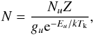 (1)where N is the total column density of the species, Z is the partition function, gu is the statistical weight of the level u, and Eu is its energy above the ground state. If optically thin, and assuming a filling factor of unity, the column density Nu is related to the observed antenna temperature:
 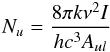 (2)where I is the integrated line intensity (in K km s-1) over frequency.
For all our analyses, where we are working with ratios of transitions with similar beams, line ratios under these approximations can be considered meaningful, and Eq. (1) is sufficient. In Table 5, we present the LTE total column densities for each species calculated for several kinetic temperatures (from 50 to 250 K, although the LTE calculations were performed from 10 to 300 K) and from each transition, for each region of the CND, as well as for the SB ring. Note that we have made the implicit assumption that all our transitions are optically thin. In reality, this is likely not the case and hence the derived LTE column densities are a lower limit: if (i) the emitting gas were in true LTE; (ii) each transition were optically thin; and (iii) the beam and velocity filling factors were the same for each transition, then the same total column density at a specific temperature should be obtainable from each transition. This is clearly not the case, and in fact differences in molecular ratios of different transitions can be quite instructive. For CO, in most cases, the differences are within an order of magnitude with the exception of the column density derived from the CO (6–5) line. At times these column densities differ by slightly more than an order of magnitude when compared with the column density derived from the J = 1–0 line, especially in the case of CND-S. However, for HCO+ and HCN the J = 4–3 transition gives a much lower column density than the J = 1–0 line, suggesting that the high J lines may be optically thick (see Sect. 3.2.1) or sub-thermally excited. From Table 5 we note that for most temperatures the E Knot is characterized by larger column densities than the other regions. Within the CND, the least chemically rich region seems to be CND-S. Nevertheless, the differences in column densities across the CND rarely exceeds one order of magnitude. In general, when comparing the CND and the SB ring in Table 5, we find that the SB ring contains gas with lower column densities by at least one order of magnitude compared to the CND, in agreement with the analysis of the molecular ratios presented in Paper I.
We may be able to better evaluate the chemical richness across the CND and potential differences between the CND and the SB ring by looking at column density ratios derived exclusively from the transitions observed with ALMA:
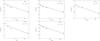 |
Fig. 7 Rotation diagrams for CO in the AGN (top left); E Knot (top middle); W Knot (top right); CND-S (bottom left); CND-N (bottom right). The black solid squares show the data with error bars, which correspond to those of the integrated intensities (errors are of the order of 10–30%). |
Within the CND: Krips et al. (2008, 2011) RADEX simulations yield an upper limit for the average kinetic temperature within the CND of 200 K; as we shall see later (see Sect. 3.2) our RADEX analysis of the individual components within the CND yields temperatures in the range of ~60–250 K. Therefore, taking an intermediate kinetic temperature of 150 K, the ratio of the CO to HCN column densities derived, respectively, from CO(3–2) and HCN(4–3) lines (whose levels have similar lower and upper energies) varies from ~2700 in the E Knot to >5000 in the W Knot, hinting at the highest and lowest abundance of the high density tracer HCN in the E Knot and W Knot, respectively. The ratio of the CO to HCO+ column densities derived from CO(3–2) and HCO+(4–3) is lowest in the E Knot (~11 700) and AGN (~13 700) and highest in the W Knot (~23 300), with the ratios in the CND-S and CND-N both quite high as well (19 500 and 17 800). Thus, the AGN and the E Knot could be the regions where most energetic activity is occurring since HCO+ can be enhanced by cosmic ray, X-ray, or UV activity.
We only have a single high J transition of CS observed with ALMA. If we make the very simplistic assumption that high J CS preferentially trace dense, shielded, and hot (due to shocks) gas, then we can use the ratio of the CO to CS column densities derived from the CO(6–5) and CS(7–6), respectively, across the CND to obtain an idea of the diversity in the hotter gas across this region. We find that this ratio is lowest for the AGN and the CND-S (~5500–6000) and highest for the E Knot (33 000), which could be an indication that the AGN and the CND-S are characterized by a high fraction of hot (shocked) gas, while the E Knot is the coolest region in the CND. Of course the above analysis is hampered by the fact that the ALMA transitions may suffer more of optical depth effects and hence the LTE approximation may be less valid.
CND vs. SB ring: Both the column density ratios, CO/HCN and CO/HCO+, estimated from the ALMA data are much higher in the SB ring, ~50 000 and ~90 000, respectively, than in the CND where the highest are ~5000 and ~23 000, respectively, indicating that both HCN and HCO+ are more abundant in the CND unless vibrational excitation by infrared photons is in fact responsible for the different ratios, a possibility we shall explore in a future paper. The fact that CO (and hence H2) is abundant but other common species remain under-abundant may be an indication that the gas has a relatively low density, traced by CO but not by higher density tracers, such as HCN and CS. This explanation would also be consistent with the relatively low HCN/HCO+ ratio found in the SB ring, with HCN being a high density tracer.
In conclusion, a simple LTE analysis provides us with the first clear indication that chemical differentiation exists across the CND and between the CND and the SB ring. In the next sub-section we present the results obtained by producing a rotation diagram of CO (for which we have four transitions) for all the regions within the CND to assess whether each sub-region of the CND can in fact be modelled by a single gas phase component.
3.1.1. CO rotation diagram
Since we have more than two CO transitions for each region within the CND, and making the assumption that LTE conditions hold, that the lines are optically thin, and that we are mostly in the Rayleigh-Jeans regime, we can use Eq. (1) to construct a rotation diagram that relates the column density per statistical weight of a number of molecular energy levels to their energy above the ground state. The assumption that the lines are optically thin may of course not be valid, especially as in dense gas the 12CO is well known to be often optically thick. The rotation diagram is a plot of the natural logarithm of Nu/gu versus Eu/k and, if the above mentioned assumptions hold, is a straight line with a negative slope of 1 /Trot. The temperature inferred from such a diagram is often referred to as the rotational temperature and it is expected to be equal to the kinetic temperature if all the levels are thermalized (Goldsmith & Langer 1999).
Figure 7 shows the rotation diagrams (with error bars – note that the errors are the absolute uncertainty in a natural log of Nu/gu) for each of our regions, namely, E Knot, W Knot, AGN, CND-N, and CND-S. The uncertainties were calculated (via standard propagation of errors) assuming the error on the level column densities are 10% for the first two transitions, 15% for the J = 3–2, and 30% for the highest J. Deviations from these errors would not be large enough to dramatically change the results. The derived rotational temperatures are, 58 K, 41 K, 50 K, 52 K, and 37 K, respectively. The errors on the rotational temperatures are around 5–7 K. However, the AGN and CND-S regions may be better represented by a two-component fit (not shown), which yields 25 K and 67 K for the AGN region, and 15 K and 54 K for the CND-S region. The rotational temperatures derived from the rotation diagrams ought to be considered as lower limits of the excitation and kinetic temperatures (Goldsmith & Langer 1999). The CO column density can also be quantified using the rotation diagram: we find that the CND-N and CND-S have the lowest CO column density at ~2–3 × 1016 cm-2, while the AGN, the W Knot, and the E Knot CO column densities are 3 × 10¹⁶, 5 × 10¹⁶ and 7 × 1016 cm-2, respectively. Compared to the values from Table 5, they are at least one order of magnitude lower. This can be due to a combination of effects: firstly, referring to Eq. (24) in Goldsmith & Langer (1999) and assuming optically thin emission, this would lead to the ordinate of the rotation diagram to be considerably below its correct value (Goldsmith & Langer 1999). Secondly, as already mentioned, a single component does not always fit the data; taking into consideration a two-component fit would boost the column density in all cases. The main conclusion to take away from this rotation diagram analysis is that, even within each region of the CND, the gas can not be characterized by a single phase.
3.2. RADEX analysis of the CND
Krips et al. (2011) performed an extensive and detailed analysis of the northern region of the CND with the radiative transfer code RADEX developed by van der Tak et al. (2007). They used the ratios of several transitions of CO, HCN, and HCO+ and found the molecular gas to be quite warm (Tkin ≥ 200 K) and dense (n(H2) ~ 104 cm-3).
In this section, in a similar manner to Krips et al. (2011), we perform a RADEX analysis with all the available molecular ratios for each region of the CND. Such modelling is limited by the assumption that all the molecular transitions sample the same gas. Although we adopt such an assumption by definition, we note that this assumption is crude, given the different critical densities of the available transitions, together with different physical and energetic conditions required for each chemical species to form (see Sect. 4). Nevertheless, if variations in temperature and density within each sub-region of the CND are not too steep, a RADEX analysis should still be able to give us an indication of the average gas density and temperature and the likely range of column densities present.
In order not to duplicate the Krips et al. (2008, 2011) analyses, we shall not discuss in detail the results of each simulation, nor the “goodness” and limitations of the best χ2 fit(s). Rather we will concentrate on the differences in the physical characteristics among the sub-regions of the CND obtained from the best RADEX fits.
RADEX offers three different possibilities for the escape probability method: a uniform sphere, an expanding sphere (LVG), and a plane parallel slab. We used all three methods but, like Krips et al. (2011), we did not find significant differences for the best fits; we therefore present the results from uniform sphere models. The collisional rates used for the RADEX calculations were taken from the LAMBDA database (Schöier et al. 2005) and are computed with a H2 as collisional partner. We have used a background temperature of 2.7 K; this may not be completely appropriate for the AGN region.
We have performed three different grids of models, which we discuss in the next three sub-sections.
3.2.1. CO fitting
We first used all our CO data as well as the 12CO/13CO line intensity ratios of 14, 10, and 14 for the CO(1–0), CO(2–1), and CO(3–2) transitions taken from Papadopoulos & Seaquist (1999). The isotopic line intensity ratios were measured with a very large beam of 14–21′′ (>950 pc), and are hence averages for the entire CND. By adopting the same 12CO/13CO line intensity ratio for each region within the CND, we are favouring, a priori, a common opacity that may not be a valid assumption (see below). As an intrinsic 12C/13C ratio we used 40; this ratio is well known to vary across clouds within our Galaxy (e.g. Milam et al. 2005), as well among galaxies (e.g. Henkel et al. 2014). For NGC 1068, Aladro et al. (2013) finds an upper limit to the isotopic ratios 12C/13C of 49, while Krips et al. (2011) find a ratio of 29. We did vary this ratio for a subset of our RADEX grid and did not find large enough differences to substantially change our conclusions.
We construct a large grid of spherical models with the following parameters:
-
1.
Gas density: n(H2) = 103–107 cm-3.
-
2.
Kinetic temperature: Tkin = 10–500 K.
-
3.
Column density/line-width: N(12CO)/ΔV = 1014–1020 cm-2/km s-1.
For a total of over 14 000 models.
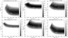 |
Fig. 8 χ2 fit results from the RADEX CO simulations of the excitation conditions within the E Knot (top left), W Knot (top middle), AGN (top right), CND-S (bottom left) and CND-N (bottom middle and right). |
We use all possible combinations of independent CO ratios: 2–1/1–0; 3–2/1–0; 6–5/3–2, 12CO(1–0)/13CO(1–0), 12CO(2–1)/ 13CO(2–1), and 12CO(3–2)/13CO(3–2). Using all the available interferometric data has the advantage that we have more ratios than parameters to fit, but has the disadvantage that the ALMA observations used for the ratios involving the 3–2 and the 6−5 lines are degraded to a linear resolution of ~100 pc. Within such a region it is very unlikely that we have a single homogeneous gas component: here we are deriving an average of the gas density and temperature provided that all the transitions used are tracing similar gas components within the ~100 pc beam. We shall always report results from a reduced χ2 fitting, where, K, the number of degrees of freedom is taken to be equal to N − n where N is the number of intensity ratios, and n is the number of fitted parameters; to be accurate, our reduced χ2 is in fact strictly speaking not a standard χ2 but a minimization function that we define as: ![Mathematical equation: \begin{eqnarray} \chi^{2}_{\rm red} = \frac{1}{K}\sum\limits_{i=1}^6[\log(R_{\rm o})-\log(R_{\rm m})]^2/\sigma^2 \end{eqnarray}](/articles/aa/full_html/2014/10/aa24116-14/aa24116-14-eq93.png) (3)where Ro and Rm are the observed and modelled ratio, respectively, and σ represents the uncertainty of the observed ratio.
(3)where Ro and Rm are the observed and modelled ratio, respectively, and σ represents the uncertainty of the observed ratio.
Examples of the best fits are shown in Fig. 8. Table 6 summarizes the best fit CO column densities (divided by the line-width), gas density and gas kinetic temperatures for each region within the CND.
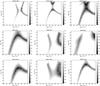 |
Fig. 9 Log of χ2 fits results from the RADEX simulations of the excitation conditions within the E Knot (top left and middle), the W Knot (top right), the AGN (middle row), the CND-S (bottom left and middle), the CND-N (bottom right) using all the available transitions. |
The opacity regimes probed by our RADEX solutions vary among the regions but also within the best density and temperature solutions: for example in the E Knot, the best fit model plotted in Fig. 8 (top left), for a density of 105 cm-3 and a temperature of 60 K, gives an opacity, τ, of ~0.2 for the J = 1–0 line (which may be surprising given the low 12/13CO (1–0) observed ratio) to a τ of just below 2 for J> 4. Towards the AGN, on the other hand, the best fit model plotted in Fig. 8 (top right), gives an opacity, which is still low for the J = 1–0 line, but up to close to six for the 6–5 line for temperatures of the order of 200 K and densities of the order of 105 cm-3. The RADEX solutions confirms what we found via the rotation diagram, namely that not all our transitions for each position are optically thin and that a single gas-phase component is not sufficient to match all the CO transitions within each sub region of the CND.
Although the conclusions we can draw from these fits are qualitative in nature, we find: i) for all the regions, but the E Knot, within the CND, the gas is hot with an average Tk> 150 K. These high temperatures are probably a consequence of X-rays or cosmic rays, and/or mechanical heating as it is unlikely that the UV would penetrate sufficiently within the gas to heat it to such high average temperatures. In fact, for cosmic rays alone to heat the gas to such temperatures, ionization rates ought be as high as 10-14 s-1 (Bayet et al. 2011) or even 10-13 s-1 (Meijerink et al. 2011). The E Knot seems to have the lowest temperature (<80 K). The hottest components are the W Knot, the AGN and, according to one solution (see Fig. 8, bottom middle panel), the CND-N; ii) although the gas densities for each component are less well constrained than the temperatures, the gas in the CND is on average dense (>104 cm-3), in agreement with the findings by Krips et al. (2011); iii) the column densities for CO are around 1017–1019 cm-2.
3.2.2. A RADEX grid computed with multi-species ratios
We now, independently, attempt to find the best density and temperature of the gas using ratios of all the available molecules and their isotopes. For our first grid we use all the independent ratios: CO(2–1/1–0); CO(3–2/1–0); CO(6–5/3–2); 12CO(1–0)/13CO(1–0), 12CO(2–1)/13CO(2–1), 12CO(3–2)/13CO(3–2), HCN(4–3/1–0), HCO+(4–3/1–0), CS(7–6/2–1), HCN(4–3)/HCO+(4–3), HCN(4–3)/CO(3–2), CS(7–6)/CO(3–2), H12CO+(1–0)/H13CO+(1–0), and H12CN(1–0)/ H13CN(1–0). We used the same line H12CN(1–0)/H13CN(1–0) and H12CO(+1–0)/H13CO+(1–0) ratios of 18 and 24, respectively (Papadopoulos & Seaquist 1999; Usero et al. 2004; Usero, priv. comm.) for each region within the CND. In order to use four different species, we need to constrain a set of parameters, namely the CO column density and the ratios among molecular abundances. We varied the gas density and temperature as in our first RADEX grid in Sect. 3.2.1 for several molecular column density ratios (see Table 7) spanning from N(CO)/ΔV = 5 × 10¹⁵ to 1018 cm-2/km s-1, N(HCO+)/ΔV = 1010 to 1013 cm-2/km s-1, N(HCN)/ΔV = 1011 to 1014 cm-2/km s-1, N(CS)/ΔV = 1011 to 1014 cm-2/km s-1 (resulting in a grid of over 10 000 models). We define a set of models to be a sub-grid of the same individual column densities for each linewidth. Of course, these sets are not exhaustive and do not cover all the possible column densities ratios, but they were guided by the range of column densities derived in LTE. As for the previous RADEX grid, we shall not discuss the results in detail, as similar RADEX analyses have been performed by Krips et al. (2008, 2011) and our average densities and temperatures confirm their general conclusions. Here we mainly concentrate on variations within the CND. However, we note that our reduced χ2 fits are much poorer than those obtained for the CO fits, an indication of the presence of multiple gas components within each region. Hence, for this RADEX grid we shall report results from the log of the reduced χ2 fitting. We note also that for each region, we always obtain more than one solution in density and temperature for the same set of column densities (see later), as well as the same density and temperature for more than one set of column densities.
Table 8 reports a summary of all our results and Fig. 9 shows our best fits. We discuss region by region below.
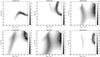 |
Fig. 10 Log of reduced χ2 fits results from the RADEX simulations of the excitation conditions within the E Knot (top left and middle), the W Knot (top right and bottom left), the AGN (bottom middle), the CND-S (bottom right) using ALMA data only (apart from one isotopic ratio – see text). |
For the E Knot Sets 1, 2, 6, and 7 (see Table 7) give the same reduced χ2 (see Fig. 9); one of the results from the RADEX CO analysis was that the best fit gas densities were always above 104 cm-3: we therefore use this lower limit as a further constraint and we are left with Sets 1 and 7, because the others all give gas densities below 104 cm-3. Set 7 gives multiple solutions in the nH − Tk plane: the high temperature (~400 K) solution, although in agreement with the RADEX results from Krips et al. (2011; which was however an average across a larger area), is the less likely given the findings from the CO RADEX analysis. For the W Knot Set 7 has the lowest reduced χ2 fit, with gas density and temperature solutions consistent with the CO RADEX analysis. For the AGN, Sets 3, 6, and 7 yield the same reduced χ2 and more than one solution in the density-temperature plane. For the CND-S, Set 2 and Set 7 yield the best fits. Finally, for the CND-N only Set 7 provides the best fit.
All regions, but the CND-N and the W Knot, can be fitted by more than one set, but equally, all regions can be fitted by the same set, implying that we cannot exclude that all the regions are chemically similar, with common ratios of HCN/HCO+ = 100, CO/HCN = 104, CO/HCO+ = 106, and CO/CS = 105. In this scenario, we note that the HCN/HCO+ abundance ratio is very high compared to those found in extragalactic environments, although chemically an abundance ratio of 100 is in fact feasible in both dense (104 cm-3) PDR gas and star forming (nH ≥ 105 cm-3) gas (Bayet et al. 2008, 2009), because of the high abundance of HCN. Hence, it may be an indication of very dense gas present. We also find that the AGN and the CND-N are the hottest regions and that the lowest limit for the gas density is 105 cm-3. We note again here that vibrational excitation by infrared photons may provide an alternative explanation for the observed ratios in this hot gas. In fact, several authors, (e.g. Sakamoto et al. 2010), found that HCN, and possibly other species, including HCO+ and CO, can be excited by infrared pumping in AGN- or starburst-dominated galaxies, and very recently, González-Alfonso et al. (2014) reported far-infrared pumping of H2O by dust in NGC 1068. If one takes into consideration the CO column densities as derived by the RADEX CO only analysis, then Set 1 is the best fit for the E Knot, while both Set 6 and 7 fit the AGN well, with Set 6 yielding a higher average density and temperature, that may be more consistent with the environment of the AGN. In this scenario, the chemical ratios for the E Knot are 10, 5 × 10⁴, 5 × 10⁵, and 5 × 10⁴ for HCN/HCO+, CO/HCN, CO/HCO+, and CO/CS, respectively, while for the AGN they are 10, 104, 105, and 104.
This excitation analysis does not allow us to distinguish whether the differences in intensity ratios across the CND are due to different energetics or simply differences in the density of the regions. We again underline that we have used a large number of ratios involving several transitions for which we only had low resolution data (100 pc and lower) and the ALMA data were all degraded to 100 pc resolution. In particular, the use of the CS(7–6)/(2–1) ratio is dubious considering that the CS(2–1) observations were obtained with a beam three times the average of that for the other lines (see Table 1). Ultimately, that this analysis does not conclusively reveal a chemical differentiation may just be a consequence of the fact that it uses data with a degraded resolution, while in fact the observed molecular line ratios show dramatic changes of up to an order of magnitude inside the CND on the spatial scales probed by ALMA (see Paper I). Hence, in the next section, we reduce the number of molecular ratios to those obtained at the highest spatial resolution in our analysis to test the robustness of our results so far.
3.2.3. RADEX analysis of ALMA data only
For this grid of models, we used only ALMA data, apart from the intensities for the isotopic ratios. We used the following intensity ratios: CO(6–5/3–2); HCN(4–3)/HCO+(4–3), HCN(4–3)/ CO(3–2), CS(7–6)/CO(3–2), and 12CO(3–2)/13CO(3–2), where the latter ratio has been included to help constrain the N(X)/Δ(V). In general, we find that this grid yields a better reduced log χ2. More importantly, by reducing the size of the emission region it is more likely that the emission may arise from gas with similar physical conditions. Figure 10 and Table 9 present the best fits for four of our regions. For the CND-S, we could not perform this analysis as the CS(7–6) line intensity was too weak at its original spatial resolution. We note that (i) for this RADEX analysis the best fits are never given by a unique set; (ii) the solutions for the gas densities are all consistent with the higher end of the density solutions found from the previous multi-species RADEX analysis, and especially the CO RADEX analysis. This is consistent both with the fact that HCN and CS are tracers of high density gas (unlike CO) and with the fact that a 35 pc beam is more likely to encompass an average higher density gas than a 100 pc beam; (iii) apart from the E Knot, none of the sets producing the best fits coincide with those found in the previous RADEX analysis, again underlining the need to perform RADEX analysis with data of the same (high) spatial resolution if one wants to characterize the chemical differentiation across the CND.
For the E Knot both Set 2 and Set 7 yield a best fit (see Table 7). Both sets constrain the kinetic temperature once again to around 60 K, confirming that this region is the coolest within the CND. For the W Knot, the best fits are provided by either Set 2 or Set 6, with Set 6 yielding best fits gas density and temperature closer to the previous RADEX analyses fits; the AGN is best fitted by Set 4 and the best fit density and temperature is in agreement with previous RADEX analyses; the CND-N is best fitted by Set 3.
The column density ratios are listed in Table 9. Favouring the solutions from this analysis, we find that the AGN has the lowest CO/HCO+, CO/HCN, and CO/CS ratios; the E Knot and the W Knot have the highest CO/HCO+ and CO/HCN ratios (if Set 2 is favoured); while HCN/HCO+ is constant, at 10, across the CND with the possible exception of the E Knot where it is 100 (if Set 7 is favoured). In order to use these ratios as tracers of the dominating energetic process(es) within each CND component, they need to be compared with chemical models, as we shall do in Sect. 4. We emphasize here that, while this analysis benefitted from the use of all (but one) ratios of transitions observed at the highest spatial resolution, it still suffers from the use of a single transition for three of the four molecules. This potentially leads to biases, especially with respect to gas density estimation.
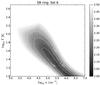 |
Fig. 11 Log of the reduced χ2 fit results from the RADEX simulations of the excitation conditions of the SB ring. |
3.3. RADEX analysis of the SB ring
For the starburst ring, only the following observations are available: CO (3–2), CO (1–0), HCO+ (4–3), HCO+ (1–0), HCN (4–3), and HCN (1–0). We therefore perform the RADEX analysis on the following ratios: CO(3–2)/(1–0), HCO+(4–3)/(1–0), HCN(4–3)/(1–0), HCN(1–0)/CO(1–0), and HCN(1–0)/HCO+(1–0), the three isotopic line intensity ratios for the CO transitions, H13CO+(1–0)/H12CO+(1–0) and H13CN(1–0)/H12CN(1–0). The isotopic ratios are again from Papadopoulos & Seaquist (1999); Usero et al. (2004; Usero, priv. comm.). We use the same sets as in Table 7 and find that the best fits are for Sets 6 (Fig. 11) and 7, both yielding a gas density ranging from 3 × 10⁴ to 3 × 106 cm-3; the temperature is less constrained with a maximum value around 60 K.
In terms of molecular ratios, if we take the results from the RADEX fit in Sect. 3.2.3, then the SB ring has similar ratios as the W Knot or the E Knot, however, with quite different physical conditions. From Fig. 11, it is clear that, once we exclude temperatures below ~30 K (the SB ring being a site of high star formation activity), then the gas density and temperature are quite well constrained to 5 × 10⁴–105 cm-3 and ~40 K.
Without high spatial resolution data for the SB ring, we cannot quantitatively determine the chemical differentiation between the CND and the SB ring, but it seems that the SB ring has an average temperature much lower than that in the CND. This implies that the differences in line intensities may be, at least partly, due to excitation effects i.e. a lower gas temperature may lead to a lower HCO+(4–3), and HCN(4–3) intensity, for example, which would justify the lower HCN(4–3)/HCN(1–0) and HCO+(4–3)/HCO+(1–0) ratios (see Table 4). A larger number of transitions at high spatial resolution will be required to determine, with RADEX, whether this scenario is valid.
4. Chemical modelling
Aladro et al. (2013) observed the nucleus of NGC 1068 with the IRAM 30-m single dish telescope in the λ ~ 3 mm range in several molecules including, CO, HCO+ and HCN. Despite the lack of spatial resolution they attempted to disentangle the different gas components and energetics with the use of time dependent gas-grain chemical and PDR models. The main conclusions of Aladro et al. (2013) were that molecules usually assumed to be PDR tracers can, in fact, also arise from dense gas that is shielded from the UV. They also found that a high cosmic ray ionization, possibly together with an enhanced (compared to a standard) radiation field, was needed to explain most of the molecular abundances. They found that shocks were not necessary, although they could not rule them out. While their modelling constrained some of the energetics, it could not provide any physical information on the different gas components. Here, we use the UCL_CHEM model (Viti et al. 2004, 2011) to determine the best physical characteristics of each individual component within the CND by comparing the ratio of theoretical column densities with the ratio of observed column densities derived from the RADEX analysis.
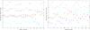 |
Fig. 12 Theoretical fractional abundances ratios for the grid of UCL_CHEM models at low AV (2 mag; left panel) and at high AV (10 mag; right panel). The black squares are CO/HCO+ ratios; red stars = CO/HCN; green crosses = CO/CS; cyan triangles = HCN/CS; blue triangles = HCN/HCO+. |
UCL_CHEM is a 1D time dependent gas-grain chemical and shock model. It is an ab initio model in that it computes the evolution as a function of time and density of chemical abundances of the gas and on the ices starting from a complete diffuse and atomic gas. For the present calculations we used the code in a single point mode (i.e. depth-independent) and was run in two Phases in time (which we shall call Phases I and II) so that: the initial density in Phase I was ~100 cm-3. During Phase I, the high density gas is achieved by means of a free-fall (or modified) collapse, in a time determined by the final density (which we varied). The temperature during this phase is kept constant at 10 K, and the cosmic ray ionization rates and radiation fields are at their standard Galactic values of ζ = 5 × 10-17 s-1 and 1 Draine, or 2.74 × 10⁻³ erg/s/cm2, respectively. Note that the collapse in Phase I is not meant to represent the formation of protostars, but it is simply a way to compute the chemistry of high density gas in a self-consistent way starting from a diffuse atomic gas, i.e. without assuming the chemical composition at its final density. In reality, we do not know how the gas reached its high density and we could have assumed any other number of density functions with time. For simplicity, we adopt free-fall collapse. Atoms and molecules are allowed to freeze onto the dust grains forming icy mantles. Non-thermal evaporation is also included (Roberts et al. 2007). Both gas and surface chemistry are self-consistently computed. Once the gas is in dynamical equilibrium again, Phase I is either allowed to continue at constant density for a further million of years, or is stopped. In Phase II, UCL_CHEM computes the chemical evolution of the gas and the dust after either an assumed burst of star formation or AGN activity has occurred. The temperature of the gas increases from 10 K to a value set by the user, and sublimation from the icy mantles occurs. The chemical evolution of the gas is then followed for about 5 × 10⁶ years. In both phases of the UCL_CHEM model, the chemical network is based on a modified UMIST data base (Woodall et al. 2007). The surface reactions included in this model are assumed to be mainly hydrogenation reactions, allowing chemical saturation when possible.
There are several free parameters involved in the setting up of chemical models. We have kept fixed the initial elemental abundances at the standard solar metallicity ISM abundances compared to the total number of hydrogen nuclei; here we list the most abundant initial elemental abundances, namely, C, O, N and S which are, respectively, 2.7 × 10⁻⁴, 4.9 × 10⁻⁴, 6.8 × 10⁻⁵ and 1.3 × 10⁻⁵; see Asplund et al. (2009) for a complete list. We then explored the parameter space for the quantities listed in Table 10. In particular, we varied:
-
1.
The final gas density at the end of the collapse. Note that for themodels where a shock is simulated this density corresponds to thepre-shock density.
-
2.
The temperature, 100 K and 200 K, during Phase II; the range of final densities and temperatures in Phase II explored reflect the best fits found in this and previous studies of NGC 1068.
-
3.
The radiation field (G°); although the range of radiation fields investigated is somewhat arbitrary, our aim was to explore the influence of relatively high values, typical of starburst galaxies, on the observed molecules, and hence we picked three representative values of a low (1 Draine), medium (10 Draine) and high (500 Draine) radiation field.
-
4.
The cosmic ray ionization rate (ζ); note that in our chemical models the cosmic ray ionization flux is also used to “mimic” an enhanced X-ray flux, which is why we choose such a large range. This approximation has its limitations because X-rays ionize and heat gas much more efficiently than cosmic rays; however, the trends in some ions, including HCO+, are the same for CRs and X-rays for a fixed gas temperature, which is what is assumed in these models.
-
5.
The length of time at which the dense gas is quiescent in Phase I, where either Phase I was stopped once the final density was reached (we shall call these the S models), or we allowed Phase I to run for a further 1–2 × 10⁶ years (L models). Phase I in the S models lasts for different times depending on the final density; for reference, 5 × 10⁶ yrs for a final density of 104 cm-3 up to 5.4 × 10⁶ yrs for a final density of 2 × 106 cm-3. However, since models differing only in this parameter gave very similar solutions we shall not discuss this parameter any further.
-
6.
Finally we also ran some models simulating the presence of shocks (in Phase II). For these models we adopted a representative shock velocity of 40 km s-1. The shocks in UCL_CHEM are treated in a parametric form as in Jimenez-Serra et al. (2008), which considers a plane-parallel C-Shock propagating with a velocity vs through the ambient medium.
Details of this version of UCL_CHEM can be found in Viti et al. (2011).
Before performing a qualitative comparison we need to note explicitly that even at the highest spatial resolution of the ALMA data, the gas is extended to ~35 pc and hence the emission cannot be from a single density component: hence we do not expect one chemical model to fit all the molecular ratios. Moreover, without any further information of the size/geometry we are constrained in using ratios of fractional abundances, which do not necessarily represent the ratio of column densities if the emission region varies from molecule to molecule. Hence, we ran each model for different sizes to achieve two representative visual extinctions of 2 and 10 mag, for the same gas density. The exact choice of Av is not important for these calculations because we are then using column density ratios. However, it is important to choose an Av below and one above the typical extinction at which the gas is shielded by UV radiation. Note that all the analysis and comparisons of the abundances from the chemical models are performed at the last time step of Phase II. In fact, as discussed later, and as also discussed in Aladro et al. (2013) and more generally in Bayet et al. (2008) and Meijerink et al. (2013), the effects of time dependence cannot be ignored in energetic extragalactic environments such as AGNs.
We shall now compare theoretical ratios (in log in Fig. 12) with the RADEX solutions from Sect. 3.2.2 as well as Sect. 3.2.3. As the chemical model is single point, we estimated the theoretical column densities, a posteriori, from the fractional abundances using the “on the spot” approximation:  (4)where Av is the visual extinction and N(H2) is equal to 1.6 × 1021 cm-2, the hydrogen column density corresponding to AV = 1 mag (Dyson & Williams 1997). Hence, the column density derived is not cumulative, but the column density at a particular visual extinction. Of course, the derived and cumulative column densities would be equivalent if the fractional abundance of species X were the same at all the Av (which is not the case). In Fig. 12 the left and right panels correspond to models ran at low and high Av, respectively. It is worth noting that since we are using logarithmic values of column density ratios, we are “insensitive” to small differences. Note also that Models 25–27 are not shown in the figure, but will be discussed below.
Our multi-species RADEX analyses give several possible solutions for the molecular line ratios (e.g. Table 8), which we will now compare with the grid of chemical models from Fig. 12. We report our results in Tables 11 and 12, where we compare the log of the molecular ratios from our chemical models with the solutions from Sects. 3.2.2 and 3.2.3, respectively.
Tables 11 and 12 are hard to interpret because not only can each region be fitted by more than one set of column densities but also, as expected, there is no one single model that can explain the set of all ratios; this is of course consistent with the fact that we need more than one gas component to characterize each sub-region. We now attempt to remove some of the chemical model solutions by taking into consideration the density constraints provided by the RADEX analyses: the latter analysis exclude a density ≤104 cm-3, therefore, we shall exclude a priori all models with a gas density of 104 cm-3. For the matching of the ratios involving HCO+, we shall also exclude chemical models where neither the radiation field nor the cosmic ray ionization rate are enhanced: this implies that the CO/HCO+ abundance ratio in all regions can be matched by Model 9 for Set 7. The ratio in the E Knot can also be matched by Model 5 for Sets 1 or 2, and in the W Knot and the CND-S by Model 5 for Set 2; and, finally, for the AGN by Model 15 for Set 4. The other ratio involving HCO+ is the HCN/HCO+ ratio: this ratio can only be matched by Model 15 for all our regions with different sets, implying that the gas emitting HCO+ in the CND must be subjected to an enhanced cosmic ray ionization field but that it must also be quite dense. We note that Set 7 cannot match the CO/HCN ratio, which is well matched by Model 15 for all our regions but, again, for different sets. The CO/CS can only be matched by models with high temperatures (24 for the E Knot with Set 1, and 18 or 24 for the AGN for Sets 3 or 6) or very high densities (e.g. Model 6 for the CND-S for Set 2). The HCN/CS ratio, for most best fit models, seems to require the presence of shocks i.e. if HCN and CS are co-spatial then shocks must be invoked. The presence of shocks is consistent with the findings from Paper I. Considering the many possible combinations of chemical sets and chemical models one can have for each sub-region we cannot draw any further conclusions. Nevertheless, the message that can be extracted from our chemical modelling is that the chemistry is not the same in every sub-region of the CND, and that provided there is chemical differentiation across the CND then a simplified picture with three dominant gas phases emerges for all regions: a “low” density (105 cm-3) region, and a higher density (≥106 cm-3) region, both with a cosmic ray ionization rate (and/or X-ray activity) enhanced by a least a factor of 10, as well as a component of shocked gas. We cannot draw conclusions on differences in gas densities, temperatures or energetics within the CND from this preliminary modelling. While it may not be surprising that the chemistry differs across the CND, this is the first chemical study that, using high spatial resolution observations coupled with a chemical model that includes gas-grain interactions, explicitly disentangles the different chemistries, albeit in a qualitative manner.
Summary of the best fit chemical model(s) for the molecular ratios in the different components in the CND using the best fit RADEX solutions from Sect. 3.2.3.
There are several caveats that should be considered when comparing chemical models with RADEX results. Firstly, while RADEX provides a solution for the average density and temperature, these chemical models calculate the chemistry at a fixed, homogeneous density, and temperature. Therefore they do not calculate the average molecular ratios across the regions, but the molecular ratio at a particular density, visual extinction, and temperature. Hence it is reasonable to employ multiple chemical models to reproduce the chemical composition of our gas. Secondly, as RADEX is an excitation and radiative transfer model, the chemical effects of an enhanced UV, cosmic ray or X-ray irradiation on the chemistry are “embedded” in the input column densities. While we have not, by any means, exhausted the parameter space of chemical modelling, we confirm that within each CND component more than one gas phase is present and that more transitions of the same species need to be observed with ALMA resolution to determine the physical characteristics across the CND with confidence. Moreover, we note that the models used here are time dependent, while we only compared ratios at chemical equilibrium. In fact, some of our ratios, in particular HCN/HCO+, are well known to be very time dependent in both dense gas (see Fig. 1 from Bayet et al. 2008) as well as in X-ray dominated environments, such as AGNs, (see Meijerink et al. 2013) so multiple gas phases can co-exist spatially and temporally. This attempt at chemical modelling was preliminary and a proper theoretical investigation including PDR, gas-grain, and XDR models will be presented in a forthcoming paper.
5. Conclusions
We performed a chemical analysis of the dense gas within the CND and the SB ring with the aim of quantifying the chemical differentiation across the CND, and we attempt a determination of the chemical origin of such differentiation. From our analysis we can draw the following conclusions:
-
A simple LTE analysis shows that: the E Knot has aricher molecular content than the rest of the CND, and the leastchemically rich region is CND-S. The SB ring hasa lower molecular content than the CND. From the CO/HCNratios, as derived from the transitions observed with ALMA, wemay deduce that the E Knot is the most abundant inhigh density molecular tracers, while the W Knotis the least abundant; from the CO/HCO+ ratio, we see that the AGN and the E Knot are the regions where most energetic activity is happening; from the CO/CS high J column density ratio, we also deduce that the E Knot may be the coolest region, while the AGN and the CND-S may be the hottest.
-
A rotation diagram analysis of CO leads to the following rotational temperatures: 58 K, 41 K, 50 K, 52 K, and 37 K for the E Knot, W Knot, AGN, CND-N, and CND-S, respectively, with typical errors of 5–7 K. The rotational temperatures are lower limits, assuming that the emission is optically thin and in LTE.
-
A RADEX analysis of the CO ratios, including rare isotopologues, indicates that the lowest temperature component within the CND is the E Knot, which also has the lowest CO column density. The AGN, the W Knot, and possibly the CND-N positions have the highest temperatures (Tk> 150 K). The average gas density is always above 104 cm-3.
-
A RADEX analysis of all the independent ratios with the species CO, HCN, HCO+, and CS gives multiple solutions in terms of column densities as well as densities and temperatures. From this analysis alone we cannot discern whether the differences in molecular ratios across the CND are due to chemical diversity or differences in physical conditions or a combination of the two (which of course are not independent).
-
A RADEX analysis performed with a reduced number of ratios using only ALMA data at the highest spatial resolution gives better contraints, in particular in terms of absolute values for the column densities, although the E Knot and the W Knot still have multiple solutions for the ratios of column densities. With this analysis, we confirm our LTE findings that the AGN has the lowest CO/HCO+, CO/HCN, and CO/CS ratios, while the E Knot and W Knot have the highest CO/HCO+ ratio and the W Knot, and possibly the E Knot, have the highest CO/HCN ratio. This analysis yields a lower limit for the gas density of 5 × 105 cm-3 for the E Knot and higher densities for all the other components. The hottest region is the AGN, while the coolest is the E Knot.
-
A RADEX analysis of the SB ring leads to the conclusion that it may be chemically similar to the W Knot, but with substantially lower gas density and temperature.
-
Finally, we attempt to determine the main driver of the chemistry in the CND with a time dependent gas-grain chemical models, UCL_CHEM. We compare a relatively large grid of chemical models with solutions provided by the RADEX grids. This comparison proves to be rather difficult and does not lead to any strong quantitative conclusion. However, chemical modelling seems to indicate that there has to be a pronounced chemical differentiation across the CND and that each sub-region could be characterized by a three-phase component ISM. In this scenario, we find that two of the gas phases are at different densities but are both subjected to a high ionization rate, and one gas component is comprised of shocked gas where most likely the CS (and possibly some of the HCN) arises from.
In conclusion, the LTE, RADEX, and chemical analysis all indicate that more than one gas-phase component is necessary to fit all the available molecular ratios uniquely. With the improved spatial resolution of ALMA, we expect this result to be confirmed by studies of other extragalactic systems also. Chemically this is certainly not unexpected. For example, HCO+ is usually the product of ion-molecule reactions involving C+ and CO+. These ions are only abundant in regions where CO can efficiently dissociate via reactions with He+; while high fluxes of cosmic and/or X-rays can lead to a high ionization fraction even in dense environments, usually they also lead to low abundances of HCN and CS (e.g. Bayet et al. 2011). Even for the same molecular species, radiative transfer studies of multi-transition observations of nearby starburst galaxies have shown that different J lines will peak at different gas densities and temperatures. Hence, our somewhat degenerate results are consistent with multiple gas phases spatially and temporally co-existing. Finally, we emphasize that this analysis did not take into consideration infrared pumping, which in fact may be responsible for the excitation of several of the observed transitions, as has been recently shown to be the case for high-lying H2O lines (González-Alfonso et al. 2014).
It is clear from our preliminary analysis that a higher number of molecular transitions, including vibrationally excited transitions, at ALMA resolution is necessary to determine the chemical and physical characteristics of each sub-region within the CND. In a future paper, we shall attempt a more thorough modelling, that will include 2D maps as well as principal component analysis to investigate the relationship between the different species across the structures in the maps, as well as a detailed analysis of the individual spectra with the use of a larger suite of chemical, PDR, XDR and non LVG line radiative transfer models.
Online material
Total beam averaged column densities (in cm-2) for CO, HCO+, HCN, and CS derived using single transitions for a range of temperature assuming LTE and optically thin emission for the CND components, as well as for the SB ring.
Physical and chemical characteristics of the five selected sub-regions within the CND (see Fig. 6) as derived by a RADEX analysis of the CO emission only.
The seven sets of RADEX models using all available transitions. Columns 2–5 are the adopted column densities, in units of cm-2 where a(b) stands for a × 10b.
Physical and chemical characteristics of the five sub-regions within the CND as derived by a RADEX analysis of the all the available independent ratios, and using the lower limit of the gas density as derived by the CO RADEX fitting as a constraint.
Physical and chemical characteristics of the five sub-regions within the CND as derived by a RADEX analysis of only the high resolution ALMA ratios, and using the lower limit of the gas density as derived by the CO RADEX fitting as a constraint.
Grid of chemical models.
Summary of the best fit chemical model(s) for the molecular ratios as derived from the RADEX analysis in Sect. 3.2.2.
Acknowledgments
We thank the staff of ALMA in Chile and the ARC-people at IRAM-Grenoble in France for their invaluable help during the data reduction process. A.U. and P.P. acknowledge support from Spanish grants AYA2012-32295 and FIS2012-32096. This paper makes use of the following ALMA data: ADS/JAO.ALMA#2011.0.00083.S. ALMA is a partnership of ESO (representing its member states), NSF (USA) and NINS (Japan), together with NRC (Canada) and NSC and ASIAA (Taiwan), in cooperation with the Republic of Chile. The Joint ALMA Observatory is operated by ESO, AUI/NRAO and NAOJ. The National Radio Astronomy Observatory is a facility of the National Science Foundation operated under cooperative agreement by Associated Universities, Inc. Some of the observations used were carried out with the IRAM Plateau de Bure Interferometer. IRAM is supported by INSU/CNRS (France), MPG (Germany) and IGN (Spain). S.G.B. and I.M. acknowledge support from Spanish grants AYA2010-15169, AYA2012-32295 and from the Junta de Andalucia through TIC-114 and the Excellence Project P08-TIC-03531. S.G.B. and A.F. acknowledge support from MICIN within program CONSOLIDER INGENIO 2010, under grant “Molecular Astrophysics: The Herschel and ALMA Era–ASTROMOL” (ref. CSD2009-00038).
References
- Aalto, S., Costagliola, F., van der Tak, F., et al. 2011, A&A, 527, A69 [NASA ADS] [CrossRef] [EDP Sciences] [Google Scholar]
- Aalto, S., García-Burillo, S., Muller, S., et al. 2012, A&A, 537, A44 [NASA ADS] [CrossRef] [EDP Sciences] [Google Scholar]
- Aladro, R., Viti, S., Bayet, E., et al. 2013, A&A, 549, A39 [NASA ADS] [CrossRef] [EDP Sciences] [Google Scholar]
- Asplund, M., Grevesse, N., Sauval, A. J., & Scott, P. 2009, ARA&A, 47, 481 [NASA ADS] [CrossRef] [Google Scholar]
- Bayet, E., Viti, S., Williams, D. A., & Rawlings, J. M. C. 2008, ApJ, 676, 978 [NASA ADS] [CrossRef] [Google Scholar]
- Bayet, E., Viti, S., Williams, D. A., Rawlings, J. M. C., & Bell, T. 2009, ApJ, 696, 1466 [NASA ADS] [CrossRef] [Google Scholar]
- Bayet, E., Williams, D. A., Hartquist, T. W., & Viti, S. 2011, MNRAS, 414, 627 [NASA ADS] [CrossRef] [Google Scholar]
- Cicone, C., Maiolino, R., Sturm, E., et al. 2014, A&A, 562, A21 [NASA ADS] [CrossRef] [EDP Sciences] [Google Scholar]
- Combes, F. 2006, Astrophys. Update, 2, 159 [NASA ADS] [CrossRef] [Google Scholar]
- Combes, F., García-Burillo, S., Casasola, V., et al. 2013, A&A, 558, A124 [NASA ADS] [CrossRef] [EDP Sciences] [Google Scholar]
- Costagliola, F., Aalto, S., Rodriguez, M. I., et al. 2011, A&A, 528, A30 [NASA ADS] [CrossRef] [EDP Sciences] [Google Scholar]
- Dyson, J. E., & Williams, D. A. 1997, The Physics of the Interstellar Medium (Taylor & Francis) [Google Scholar]
- Feruglio, C., Maiolino, R., Piconcelli, E., et al. 2010, A&A, 518, A155 [Google Scholar]
- Fuente, A., García-Burillo, S., Usero, M., et al. 2008, A&A, 492, 675 [NASA ADS] [CrossRef] [EDP Sciences] [Google Scholar]
- García-Burillo, S., Martín-Pintado, J., Fuente, A., Usero, A., & Neri, R. 2002, ApJ, 575, L55 [NASA ADS] [CrossRef] [Google Scholar]
- García-Burillo, S., Combes, F., Gracía-Carpio, J., et al. 2008, A&AS, 313, 261 [Google Scholar]
- García-Burillo, S., Usero, A., Fuente, A., et al. 2010, A&A, 519, A2 [NASA ADS] [CrossRef] [EDP Sciences] [Google Scholar]
- García-Burillo, S., Combes, F., Usero, A., et al. 2014, A&A, 567, A125 (Paper I) [NASA ADS] [CrossRef] [EDP Sciences] [Google Scholar]
- Goldsmith, P. F., & Langer, W. D. 1999, ApJ, 517, 209 [NASA ADS] [CrossRef] [Google Scholar]
- González-Alfonso, E., Fischer, J., Aalto, S., & Falstad, N. 2014, A&A, 567, A91 [NASA ADS] [CrossRef] [EDP Sciences] [Google Scholar]
- Hailey-Dunsheath, S., Sturm, E., Fisher, J., et al. 2012, ApJ, 755, 57 [NASA ADS] [CrossRef] [Google Scholar]
- Henkel, C., Asiri, H., Ao, Y., et al. 2014, A&A, 565, A3 [NASA ADS] [CrossRef] [EDP Sciences] [Google Scholar]
- Israel, F. P. 2009, A&A, 493, 525 [NASA ADS] [CrossRef] [EDP Sciences] [Google Scholar]
- Jimenez-Serra, I., Caselli, P., Martín-Pintado, J., & Hartquist, T. W. 2008, A&A, 482, 549 [NASA ADS] [CrossRef] [EDP Sciences] [Google Scholar]
- Kamenetzky, J., Glenn, J., Maloney, P. R., et al. 2011, ApJ, 731, 83 [NASA ADS] [CrossRef] [Google Scholar]
- Krips, M., Neri, R., García-Burillo, S., et al. 2008, ApJ, 677, 262 [NASA ADS] [CrossRef] [Google Scholar]
- Krips, M., Martín, S., Eckart, A., et al. 2011, ApJ, 736, 37 [NASA ADS] [CrossRef] [Google Scholar]
- Loenen, A. F., Spaans, M., Baan, W. A., & Meijerink, R. 2008, A&A, 488 [Google Scholar]
- Martín, S., Krips, M., Martín-Pintado, J., et al. 2011, A&A, 527, A36 [NASA ADS] [CrossRef] [EDP Sciences] [Google Scholar]
- Meier, D. S., & Turner, J. L. 2005, ApJ, 618, 259 [NASA ADS] [CrossRef] [Google Scholar]
- Meier, D. S., & Turner, J. L. 2012, ApJ, 755, 104 [NASA ADS] [CrossRef] [Google Scholar]
- Meijerink, R., & Spaans, M. 2005, A&A, 436, 397 [NASA ADS] [CrossRef] [EDP Sciences] [Google Scholar]
- Meijerink, R., Spaans, M., & Israel, F. P. 2007, A&A, 461, 793 [NASA ADS] [CrossRef] [EDP Sciences] [Google Scholar]
- Meijerink, R., Spaans, M., Loenen, A. F., & van der Werf, P. P. 2011, A&A, 525, A119 [NASA ADS] [CrossRef] [EDP Sciences] [Google Scholar]
- Meijerink, R., Spaans, M., Kamp, I., et al. 2013, J. Phys. Chem. A, 117, 9593 [CrossRef] [Google Scholar]
- Milam, S. N., Savage, C., Brewster, M. A., et al. 2005, ApJ, 634, 1126 [NASA ADS] [CrossRef] [Google Scholar]
- Omont, A. 2007, Rep. Prog. Phys., 70, 1099 [NASA ADS] [CrossRef] [Google Scholar]
- Papadopoulos, P. P., & Seaquist, E. R. 1999, ApJ, 516, 114 [NASA ADS] [CrossRef] [Google Scholar]
- Roberts, J. F., Rawlings, J. M. C., Viti, S., & Williams, D. A. 2007, MNRAS, 382, 733 [NASA ADS] [CrossRef] [Google Scholar]
- Sakamoto, S., Aalto, S., Evans, A. S., et al. 2010, ApJ, 725 [Google Scholar]
- Schinnerer, E., Eckart, A., Tacconi, L., et al. 2000, ApJ, 533, 850 [NASA ADS] [CrossRef] [Google Scholar]
- Schöier, F. L., van der Tak, F. F. S., van Dishoeck, E. F., & Black, J. H. 2005, A&A, 432, 369 [NASA ADS] [CrossRef] [EDP Sciences] [Google Scholar]
- Tacconi, L. J., Genzel, R., Blietz, M., et al. 1994, ApJ, 426 [Google Scholar]
- Tacconi, L. J., Gallimore, J. F., Genzel, R. C., et al. 1997, Ap&SS, 248, 59 [NASA ADS] [CrossRef] [Google Scholar]
- Tsai, M., Hwang, C.-Y., Matsushita, S., et al. 2012, ApJ, 746, 129 [NASA ADS] [CrossRef] [Google Scholar]
- Usero, A., García-Burillo, S., Fuente, A., Martín-Pintado, J., & Rodríguez-Fernández, N. J. 2004, A&A, 419, 897 [NASA ADS] [CrossRef] [EDP Sciences] [Google Scholar]
- Usero, A., García-Burillo, S., Martín-Pintado, J., Fuente, A., & Neri, R. 2006, A&A, 448, 457 [NASA ADS] [CrossRef] [EDP Sciences] [Google Scholar]
- van der Tak, F. F. S., Black, J. H., Schöier, F. L., Jansen, D. J., & van Dishoeck, E. F. 2007, A&A, 468, 627 [NASA ADS] [CrossRef] [EDP Sciences] [Google Scholar]
- Veilleux, S., Meléndez, M., Sturm, E., et al. 2013, ApJ, 776, 27 [NASA ADS] [CrossRef] [Google Scholar]
- Viti, S., Collings, M. P., Dever, J. W., McCoustra, M. R. S., & Williams, D. A. 2004, MNRAS, 354, 1141 [NASA ADS] [CrossRef] [Google Scholar]
- Viti, S., Jimenez-Serra, I., Yates, J. A., et al. 2011, ApJ, 740, 3 [Google Scholar]
- Wang, J. 2004, ApJ, 614, L21 [NASA ADS] [CrossRef] [Google Scholar]
- Watanabe, Y., Sakai, N., Sorai, K., & Yamamoto, S. 2014, ApJ, 788, 4 [NASA ADS] [CrossRef] [Google Scholar]
- Woodall, J., Agúndez, M., Markwick-Kemper, A. J., & Millar, T. J. 2007, A&A, 466, 1197 [NASA ADS] [CrossRef] [EDP Sciences] [Google Scholar]
- Zinnecker, H., & Yorke, H. W. 2007, ARA&A, 45, 481 [NASA ADS] [CrossRef] [Google Scholar]
All Tables
Original spatial resolution in parsecs for all (ALMA as well as PdBI) molecular transitions used in this paper.
Coordinates, and RA and Dec offsets relative to the AGN, of the five regions within the CND and the star-forming knot of the SB ring.
Molecular velocity-integrated intensities, measured in K km s-1, for each region within the CND as well as in the starburst ring.
Molecular ratios of velocity-integrated intensities (and their error in brackets – see Sect. 2.2), measured in K km s-1, rounded to the first decimal point in most cases, for each region within the CND as well as in the starburst ring.
Summary of the best fit chemical model(s) for the molecular ratios in the different components in the CND using the best fit RADEX solutions from Sect. 3.2.3.
Total beam averaged column densities (in cm-2) for CO, HCO+, HCN, and CS derived using single transitions for a range of temperature assuming LTE and optically thin emission for the CND components, as well as for the SB ring.
Physical and chemical characteristics of the five selected sub-regions within the CND (see Fig. 6) as derived by a RADEX analysis of the CO emission only.
The seven sets of RADEX models using all available transitions. Columns 2–5 are the adopted column densities, in units of cm-2 where a(b) stands for a × 10b.
Physical and chemical characteristics of the five sub-regions within the CND as derived by a RADEX analysis of the all the available independent ratios, and using the lower limit of the gas density as derived by the CO RADEX fitting as a constraint.
Physical and chemical characteristics of the five sub-regions within the CND as derived by a RADEX analysis of only the high resolution ALMA ratios, and using the lower limit of the gas density as derived by the CO RADEX fitting as a constraint.
Summary of the best fit chemical model(s) for the molecular ratios as derived from the RADEX analysis in Sect. 3.2.2.
All Figures
|
Fig. 1 CO (3–2) velocity-integrated intensity map, measured in Jy/beam km s-1 over a 460 km s-1 window, obtained with ALMA (see Paper I Fig. 4 for more details). The central position is the phase tracking center (J2000( RA◦, Dec◦) = (02h42m40 |
| In the text | |
|
Fig. 2 Left: velocity-integrated intensity ratios CO(3–2)/CO(1–0) in the CND as well as in the SB ring. Right: CO(6–5)/CO(3–2) and CO(2–1)/CO(1–0) in the CND. The filled ellipses represent the spatial resolutions used to derive the line ratio maps: 2′′ × 1.1′′PA = 22° for CO(3–2)/CO(1–0) and CO(2–1)/CO(1–0); 0.6′′ × 0.5′′PA = 60° for CO(6–5)/CO(3–2). |
| In the text | |
|
Fig. 3 Velocity-integrated intensity ratios HCN(4–3)/HCN(1–0) (left) and HCO+(4–3)/HCO+(1–0) (right) across the CND as well as in the SB ring. The filled ellipses in the lower right corners represent the spatial resolutions used to derive the line ratio maps: 6.6′′ × 5.1′′ PA = 157°, for both panels. |
| In the text | |
|
Fig. 4 Zoomed in velocity-integrated intensity ratios HCN(4–3)/HCN(1–0), HCO+(4–3)/HCO+(1–0) and CS(7–6)/CS(2–1) in the CND. The filled ellipses represent the spatial resolutions used to derive the line ratio maps: 2′′ × 0.8′′, PA = 19° for HCN(4–3)/HCN(1–0) and HCO+(4–3)/HCO+(1–0); 6.6′′ × 3.2′′ PA = 16° for CS(7–6)/CS(2–1). |
| In the text | |
|
Fig. 5 HCN(4–3)/CO(3–2), CS(7–6)/CO(3–2) and HCN(4–3)/ HCO+(4–3) velocity-integrated intensity ratios in the CND. The filled ellipses represent the spatial resolutions used to derive the line ratio maps: 0.6′′ × 0.5′′ PA = 60°, for all panels. |
| In the text | |
|
Fig. 6 HCN(1–0)/HCO+(1–0) velocity-integrated intensity ratio (left) and the HCN(1–0)/CO(1–0) velocity-integrated intensity ratio (right) in the SB ring. The filled ellipses represent the spatial resolutions used to derive the line ratio maps: 6.6′′ × 5.1′′ PA = 157°. |
| In the text | |
|
Fig. 7 Rotation diagrams for CO in the AGN (top left); E Knot (top middle); W Knot (top right); CND-S (bottom left); CND-N (bottom right). The black solid squares show the data with error bars, which correspond to those of the integrated intensities (errors are of the order of 10–30%). |
| In the text | |
|
Fig. 8 χ2 fit results from the RADEX CO simulations of the excitation conditions within the E Knot (top left), W Knot (top middle), AGN (top right), CND-S (bottom left) and CND-N (bottom middle and right). |
| In the text | |
|
Fig. 9 Log of χ2 fits results from the RADEX simulations of the excitation conditions within the E Knot (top left and middle), the W Knot (top right), the AGN (middle row), the CND-S (bottom left and middle), the CND-N (bottom right) using all the available transitions. |
| In the text | |
|
Fig. 10 Log of reduced χ2 fits results from the RADEX simulations of the excitation conditions within the E Knot (top left and middle), the W Knot (top right and bottom left), the AGN (bottom middle), the CND-S (bottom right) using ALMA data only (apart from one isotopic ratio – see text). |
| In the text | |
|
Fig. 11 Log of the reduced χ2 fit results from the RADEX simulations of the excitation conditions of the SB ring. |
| In the text | |
|
Fig. 12 Theoretical fractional abundances ratios for the grid of UCL_CHEM models at low AV (2 mag; left panel) and at high AV (10 mag; right panel). The black squares are CO/HCO+ ratios; red stars = CO/HCN; green crosses = CO/CS; cyan triangles = HCN/CS; blue triangles = HCN/HCO+. |
| In the text | |
Current usage metrics show cumulative count of Article Views (full-text article views including HTML views, PDF and ePub downloads, according to the available data) and Abstracts Views on Vision4Press platform.
Data correspond to usage on the plateform after 2015. The current usage metrics is available 48-96 hours after online publication and is updated daily on week days.
Initial download of the metrics may take a while.