| Issue |
A&A
Volume 570, October 2014
|
|
|---|---|---|
| Article Number | A109 | |
| Number of page(s) | 11 | |
| Section | Interstellar and circumstellar matter | |
| DOI | https://doi.org/10.1051/0004-6361/201423369 | |
| Published online | 31 October 2014 | |
Molecular gas associated with IRAS 10361-5830⋆
1
Instituto Argentino de Radioastronomía,
CONICET, CCT La Plata, C.C.5,
1894
Villa Elisa,
Argentina
e-mail:
This email address is being protected from spambots. You need JavaScript enabled to view it.
2
Facultad de Ciencias Astronómicas y Geofísicas, Universidad
Nacional de la Plata, Paseo del
Bosque s/n, 1900
La Plata,
Argentina
3
Departamento de Astronomía, Universidad de Chile,
Casilla 36-D Santiago, Chile
Received: 3 January 2014
Accepted: 30 June 2014
Abstract
Aims. We analyze the distribution of the molecular gas and dust in the molecular clump linked to IRAS 10361-5830, located in the environs of the bubble-shaped Hii region Gum 31 in the Carina region, with the aim of determining the main parameters of the associated material and of investigating the evolutionary state of the young stellar objects identified there.
Methods. Using the APEX telescope, we mapped the molecular emission in the J = 3−2 transition of three CO isotopologues, 12CO, 13CO and C18O, over a 1.́5 × 1.́5 region around the IRAS position. We also observed the high-density tracers CS and HCO+ toward the source. The cold- dust distribution was analyzed using submillimeter continuum data at 870 μm obtained with the APEX telescope. Complementary IR and radio data at different wavelengths were used to complete the study of the interstellar medium.
Results. The molecular gas distribution reveals a cavity and a shell-like structure of ~0.32 pc in radius centered at the position of the IRAS source, with some young stellar objects projected onto the cavity. The total molecular mass in the shell and the mean H2volume density are ~40 M⊙ and ~(1−2) × 103 cm-3. The cold-dust counterpart of the molecular shell has been detected in the far-IR at 870 μm and in Herschel data at 350 μm. Weak extended emission at 24 μm from warm dust is projected onto the cavity, as well as weak radio continuum emission.
Conclusions. A comparison of the distribution of cold and warm dust, and molecular and ionized gas allows us to conclude that a compact Hii region has developed in the molecular clump, indicating that this is an area of recent massive star formation. Probable exciting sources capable of creating the compact Hii region are investigated. The 2MASS source 10380461-5846233 (MSX G286.3773-00.2563) seems to be responsible for the formation of the Hii region.
Key words: ISM: molecules / stars: protostars / HII regions / ISM: individual objects: IRAS 10361-5830
FITS files with datacubes corresponding to 12CO, 13CO, C180 maps are only available at the CDS via anonymous ftp to cdsarc.u-strasbg.fr (130.79.128.5) or via http://cdsarc.u-strasbg.fr/viz-bin/qcat?J/A+A/570/A109
© ESO, 2014
1. Introduction
The borders of expanding Hii regions have proved to be excellent environs for the formation of dense molecular clumps where conditions for the triggering of new generations of stars are favored (Elmegreen & Lada 1977). Dense molecular clumps and cores can be studied through the line emission from low- and high-density tracers, such as CS, HCO+, and C18O (e.g., Dedes et al. 2011). The cold-dust counterparts of these dense regions, responsible for their high visual extinction, can be detected by their continuum emission at submillimeter wavelengths (Sánchez-Monge et al. 2008; Beltrán et al. 2006).
High-density clumps where star formation is active can be identified by the presence of infrared point sources whose spectral energy distributions are typical of young stellar objects (YSOs), by OH- and/or H2O-maser emission, and by bipolar outflows detected in CO, SiO y HCO+ lines (e.g., Dionatos et al. 2010).
In this paper we report on the results of a high angular resolution molecular line and dust continuum study of one of the high-density clumps identified in the environs of the bubble-shaped Hii region Gum 31. This Hii region is located in the Carina spiral arm and is excited by the open cluster NGC 3324. Distance estimates for NGC 3324 and Car OB1 are in the range 1.8−3.6 kpc (see Cappa et al. 2008 (hereafter CNAV08) and Ohlendorf et al. 2013 for a discussion of the distance of the nebula). Following Yonekura et al. (2005) and Barnes et al. (2011), we adopt a distance d = 2.5 kpc, with an uncertainty of ±0.5 kpc.
Yonekura et al. (2005) and CNAV08 analyzed the molecular environment of Gum 31 using C18O(1−0) and 12CO(1−0) line data obtained with the NANTEN telescope with an angular resolution of 2.́7. CNAV08 found an expanding molecular envelope encircling the ionized region detected in the velocity interval from –27.2 to –14 km s-1 with (7.6 ± 3.4) × 104 M⊙ (at d = 2.5 kpc) and an H2 density of 230 cm-3. The brighter CO(1−0) emission regions coincide with dense C18O(1−0) clumps identified by Yonekura et al. (2005).
Here, we investigate the distribution of the molecular gas and cold dust in clump number 6 from the list of Yonekura et al. (2005), named BYF 77 in the Census of High-and Medium-mass Protostars (ChaMP, Barnes et al. 2011). Figure 1 shows the 12CO(1−0) line emission distribution of clump 6 extracted from CNAV08 in contours and grayscale. Using CLUMPFIND algorithm, Barnes et al. (2011) detected four cores in the HCO+ data of BYF 77 obtained with MOPRA, with an angular resolution of 36′′. Yonekura et al. (2005) found the highest density section of the clump using the H13CO+ line 1.́6 to the west and south of the IRAS position. From their CO data they estimated a mean H2 column density of 12.8 × 1021 cm-2, an H2 mass of 3700 M⊙, and an H2 volume density of 1600 cm-3, adopting a radius of 1.8 pc for the clump and d = 2.5 kpc.
An infrared cluster spatially coincident with this clump was identified by Dutra et al. (2003, (DBS2008) 128), while an X-ray clustering was identified by Preibisch et al. (2014).
Cappa et al. (2008) showed that this clump coincides with a number of YSOs detected in the IRAS, MSX, and 2MASS databases, indicating that star formation is active in this area. Its location on the molecular envelope bordering Gum 31 suggests that star formation in the clump was triggered by the expansion of the Hii region. This clump coincides with IRAS 10361-5830, centered at RA, Dec(J2000) = (10h38m04.0s, –58°46′17 8), and with the IR point-like sources MSX G286.3579-00.2933, MSX G286.3747-00.2636, MSX G286.3773-00.2563, 2MASS 10375219-5847133, and 2MASS 10381461-5844416. All of these were classified as candidate YSOs based on photometric criteria and are listed in Table 3 of CNAV08. Following Yamaguchi et al. (2001), the IR luminosity of IRAS 10361-5830 is 2 × 10⁴L⊙, suggesting massive star formation.
An analysis aimed at characterizing the protostellar and young stellar population of NGC 3324 and its environs was recently performed by Ohlendorf et al. (2013), who detected a dozen infrared point sources projected onto the dense clump using the Spitzer, WISE, and Herschel databases. They found some Class I objects and concluded that MSX G286.3773-00.2563 (=J10380461-5846233) is a Class II object. The position of the candidate YSOs projected onto clump 6 identified by CNAV08 and Ohlendorf et al. (2013) is also shown with different symbols in Fig. 1.
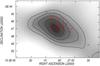 |
Fig. 1 12CO(1−0) line emission distribution toward clump number 6 from the list of Yonekura et al. (2005), in RA, Dec(J2000) coordinates, extracted from CNAV08. Contour lines go from 4.0 to 8.0 K in steps of 1 K. The 4.0 K contour delineates approximately the clump as defined in C18O. The grayscale goes from 0 to 10 K. The large square indicates the region observed in molecular lines with APEX (see Sect. 2.1). The triangle indicates the position of IRAS 10361-5530. The different symbols mark the location of candidate YSOs identified by CNAV08 and Ohlendorf et al. (2013): MSX sources (circles), 2MASS sources (crosses), Herschel sources (diamonds), and WISE sources (plus signs). |
The characteristics of this dense clump make it an interesting object in which to investigate in more detail the molecular gas and dust distribution in the environs of the candidate YSOs, with the aim of analyzing the morphology and kinematics of the associated dense gas, and achieving additional insight into the evolutionary status of the inner sources.
2. Observations
2.1. Molecular line data
To accomplish this study we surveyed a region of 90′′×90′′ centered on the IRAS position in the 12CO(3−2), 13CO(3−2), and C18O(3−2) lines using the APEX-2 (SHeFI) receiver (system temperature Tsys ~ 300 K) of the Atacama Pathfinder EXperiment (APEX) telescope, in December 2010. One single pointing was also observed toward the position of the IRAS source in the CS(7−6) and HCO+(4−3) lines. The surveyed region is indicated in Fig. 1 by the large square.
The frequency of the observed lines, the integration time τ, and the half-power beam-width (HPBW) are indicated in Table 1. The data were acquired with a fast Fourier transform spectrometer, consisting of 4090 channels, with a total bandwidth of ~800 km s-1, which provides a velocity resolution of 0.20 km s-1. The observations were performed in position-switching mode with full sampling (i.e., with a separation of 10′′). The off-source position free of CO emission is located at RA, Dec(J2000) = (10h38m53.46s, –59°18′48 6).
Calibration was performed using the planet Saturn, and the RAFGL5254 and RAFGL4211 sources. Pointing was checked twice during observations using X-TrA, Venus, and VY-CMa. The intensity calibration has an uncertainty of 10%.
The spectra were reduced using the Continuum and Line Analysis Single-dish Software (CLASS) of the Grenoble Image and Line Data Analysis Software (GILDAS)1. A linear baseline fitting was applied to the data. The root mean square (rms) noise of the profiles after baseline subtraction and calibration is listed in Table 1. The observed line intensities are expressed as main-beam brightness-temperatures Tmb, by dividing the antenna temperature  by the main-beam efficiency ηmb, equal to 0.82 for APEX-2 (Vassilev et al. 2008). The Astronomical Image Processing System (AIPS) package and CLASS software were used to perform the analysis.
Observational parameters of the rotational lines.
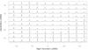 |
Fig. 2 13CO(3−2) profiles observed in a 1.́5 × 1.́5 region around IRAS 10361-5830. Each profile shows Tmb in the interval from –1 to 25 K vs. LSR velocity in the range from –30 to –15 km s-1. The (0, 0) position coincides with the position of the IRAS source in J2000 equatorial coordinates. |
2.2. Submillimeter continuum data
We also mapped the submillimeter emission in a field of 180′′× 180′′ in size centered on the IRAS position with an angular resolution of 19 2 (HPBW), using the LArge Apex Bolometer Camera (LABOCA; Siringo et al. 2009) at 870 μm (345 GHz) operating with 295 pixels at the APEX telescope. The field was observed during 1.9 h in October 2011. The atmospheric opacity was measured every 1 h with skydips. Atmospheric conditions were very good (τzenith ≃ 0.15). Focus was optimized once on Mars during observations. The absolute calibration uncertainty is estimated to be 10%. Data reduction was performed using The Comprehensive Reduction Utility for SHARC-2 software (CRUSH)2. The noise level is in the range 15−20 mJy beam-1.
2.3. Complementary data
The millimeter and submillimeter data were complemented with Spitzer images at 3.6, 4.5, 5.8, and 8.0 μm from the Galactic Legacy Infrared Mid-Plane Survey Extraordinaire (GLIMPSE; Benjamin et al. 2003), and images at 24 μm from the MIPS Inner Galactic Plane Survey (MIPSGAL; Carey et al. 2009). In addition an image at 843 MHz from the Sydney University Molonglo Sky Survey (SUMSS, Mauch et al. 2003, synthesized beam =43″ × 43″ cosec(δ)) was used.
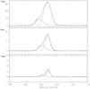 |
Fig. 3 12CO(3−2), 13CO(3−2), and C18O(3−2) averaged profiles in black lines. Gaussian fittings are overlaid in red and blue lines. The sum of the Gaussian components in each profile is shown in green. |
Parameters of the Gaussian fittings to the averaged spectra.
3. Results
3.1. Spectral analysis
Figure 2 displays the 13CO(3−2) spectra obtained for the observed region. The spatial separation between these profiles is 10′′. Relative coordinates are expressed in arcseconds, with respect to the IRAS source position, centered at RA, Dec(J2000) = (10h38m0 4, –58°46′17 8). The individual spectra exhibit two maxima with moderate emission and a separation of a few km s-1 in the central part of the observed region, while the outer regions generally show only one bright velocity component, except in the southeast section, where the two velocity components can be clearly identified.
Figure 3 displays the 12CO(3−2), 13CO(3−2), and C18O(3−2) profiles obtained by averaging the observed spectra. This allows us to distinguish the different components in the observed area and assess of the molecular gas parameters. The figure shows the excellent correspondence of the Gaussian fitting with the averaged spectra, thus indicating the presence of gas at two different velocities in the central part of the observed region. The presence of two components at different velocities in the optically thin lines 13CO(3−2) and C18O(3−2) suggests that the identification of the two components in the 12CO(3−2) spectrum is not caused by self-absorption effects.
The results are summarized in Table 2, which lists the number of Gaussian components, the peak velocity v, the velocity width at half-intensity Δv, the peak temperature Tp, and the integrated emission I (=TpΔv). Values between brackets indicate the errors in the Gaussian parameters.
The emission is concentrated between –28 and –18 km s-1, as estimated from the full width at 3σ of the averaged profiles (10 km s-1 for the 12CO(3−2) spectrum, 7 km s-1 for 13CO, and 5 km s-1 for C18O).
We adopt –25 km s-1 as the velocity of the faintest CO component and –22.8 km s-1 as the velocity of the brightest one. The remarkable decrease in intensity of this last component toward the central region in comparison with the outer regions is clear from Fig. 2. The HCO+ spectra show only one component at −22.6 km s-1, in coincidence with the brightest CO component. The HCO+ spectrum is shown in Fig. 4 overlaid with the 13CO spectrum. No CS emission was detected.
The detection of HCO+ emission and the lack of CS emission indicates a region with densities of about 106 cm-3, compatible with the critical density of HCO+ (ncrit = 1.8 × 106 cm-3).
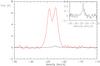 |
Fig. 4 13CO(3−2) spectrum (red) overlaid on the HCO+(4−3) spectrum (black) observed toward IRAS 10361-5830. The inset shows the HCO+ spectrum at an appropriate scale. |
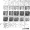 |
Fig. 5 Series of 12CO images showing the emission in the range –27.1 to –19.9 km s-1. The velocity of each panel is shown in the top-left corner of each panel. Contours go from 10 to 60 K in steps of 2 K. The central cross on each panel indicates the position of IRAS 10631-5830. The grayscale is indicated. Note that in this figure, RA increases toward the right. |
Infrared sources and candidate YSOs projected onto the observed region.
3.2. Parameters of the molecular gas: excitation temperature and optical depth
Excitation temperatures Texc and optical depths τav were estimated for the two velocity components of the CO averaged spectra. Texc was evaluated from the optically thick (τ ≫ 1) 12CO emission assuming local thermodynamic equilibrium (LTE), using the expression ![Mathematical equation: \begin{equation} T_{\rm exc} = \frac{T^*} {\ln\left[ \frac{T^*}{T^{12}_{\rm p}+T^*J(T_{\rm rad})^{-1}} + 1 \right]}, \label{eq:texc2} \end{equation}](/articles/aa/full_html/2014/10/aa23369-14/aa23369-14-eq60.png) (1)where
(1)where  ,
,  , ν32 is the frequency of the 12CO(3−2) line (345.79 GHz),
  is the peak temperature of the Gaussian in the 12CO spectrum, and Trad = 2.7 K. The error in Texc was obtained adopting an uncertainty of 10% in .
Averaged optical depths  and
and  for 12CO and 13CO, were derived using the 13CO Gaussian fitting. To estimate we used the equation
 ![Mathematical equation: \begin{equation} \tau^{13}_{\rm av} = - \ln \left[ 1 - \frac{T^{13}_{\rm p}}{T^{*}} \left[ J(T_{\rm exc})- J(T_{\rm rad}) \right]^{-1} \right], \label{eq:tau2} \end{equation}](/articles/aa/full_html/2014/10/aa23369-14/aa23369-14-eq68.png) (2)where the frequency of the 13CO(3−2) line was used in T∗.
(2)where the frequency of the 13CO(3−2) line was used in T∗.
Finally, the optical depth of the 12CO line was estimated from  (3)where Δv12 and Δv13 are the full width at half-maximum obtained from the averaged spectra, ν13 and ν12 are the frequency of the lines, and A = [12CO]/[13CO] = 70 is the isotopic ratio (Langer & Penzias 1990; Wilson & Rood 1994). Results for Texc and τav are included in the last two columns of Table 2.
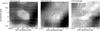 |
Fig. 6 Left panel: average 12CO line emission Tmb−12 within the velocity interval from –27.1 to –19.9 km s-1. Contours go from 14 to 24 K, in steps of 1 K. Middle panel: average image of the 13CO line emission showing Tmb−13 within the velocity interval from –27.1 to –20.8 km s-1. Contours go from 3 to 10 K in steps of 0.5 K. Right panel: average image of the C18O line emission showing Tmb−18 within the velocity interval from –25.0 to –21.1 km s-1. Contours are 0.51, 0.68, 0.85, 1.02, 1.19, 1.70, 2.04, and 2.38 K. The triangle indicates the position of IRAS 10361-5530. The different symbols mark the location of candidate YSOs identified by CNAV08 and Ohlendorf et al. (2013): MSX sources (circles) and WISE sources (plus signs). White contours in the left panel correspond to Tmb ≤ 17 K. |
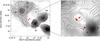 |
Fig. 7 Left panel: 870 μm continuum emission map. Dust clumps are indicated. The grayscale goes from −0.1 to 2.0 Jy beam-1. Contour levels correspond to 0.2, 0.35, 0.5, and 0.7 Jy beam-1, and from 0.75 to 2.0 Jy beam-1 in steps of 0.25 Jy beam-1. The large square indicates the region observed in CO lines and the different symbols have the same meaning as in Fig. 6. Right panel: overlay of the emission at 870 μm (grayscale) and the CO contours of Fig. 6. IR sources listed in Table 3 are indicated. |
3.3. Molecular gas distribution
To study the spatial distribution of the molecular gas, we constructed a series of images of the 12CO emission at different velocities within the velocity interval from –27.1 to –19.9 km s-1 in steps of 0.3 km s-1. These images, which are displayed in Fig. 5, show a low-emission region centered at RA, Dec(J2000) = (10h38m04s, –58°46′′24′), close to the position of the IRAS source (indicated by a cross). The cavity is completely encircled by regions of enhanced emission, defining a molecular envelope. The low-emission region displays its steeper temperature gradient at v = −22.9 ± 0.3 km s-1.
Toward more negative velocities, the cavity and envelope can be clearly followed up to –25.3 km s-1, although faint extensions are present up to –27.1 km s-1, while toward more positive velocities, they extend up to –20.8 km s-1, with weaker extensions up to –19.9 km s-1.
The structure can be imaged by averaging the 12CO emission within the velocity interval from –27.1 to –19.9 km s-1. Figure 6 (left panel) displays the main-beam brightness-temperature Tmb−12 map of the 12CO(3−2) line emission. The position of the IRAS source and the candidate YSOs from CNVA08 and Ohlendorf et al. (2013) are indicated in this figure. The coordinates and names of these sources are listed in Table 3, along with the class-type from Ohlendorf et al. (2013).
The 13CO(3−2) line emission distribution is shown in the center panel of Fig. 6, which displays the spatial distribution of Tmb−13 in the interval from –27.1 to –20.8 km s-1.
The spatial distribution of the 12CO(3−2) line emission clearly shows the area of low intensity (with Tmb−12 ≲ 17 K) centered near the position of the IRAS source, encircled by a shell-like structure. The brightest region is located at RA, Dec(J2000) = (10h37m59s, −58°46′25′′) and reaches about 24 K. Very probably, this bright region corresponds to an extension toward the west of BYF 77b identified by Barnes et al. (2011) in HCO+(1−0) lines. The envelope shows other areas of high emission located at RA, Dec(J2000) = (10h38m8s, –58°45′55′′), coincident with BYF 77c from the list of Barnes et al. (2011), and at (10h38m07s, –58°46′40′′), which have intensities of about 20 K. In this map all the emission is above the rms noise (3σprom = 0.21 K). The analysis of the 13CO(3−2) line emission distribution (Fig. 6, middle panel) leads to a similar conclusion, although in this case the envelope is not complete. Finally, denser regions in the molecular shell are detected in the C18O line (right panel).
It is important to note that the velocity range where the 12CO, 13CO and C18O emissions are detected is compatible with the velocity of the molecular gas associated with Gum 31 (CNAV08, Yonekura et al. 2005; Barnes et al. 2011), indicating that the molecular shell identified with the APEX data is linked to Gum 31. In particular, the velocity of BYF77 derived by Barnes et al. (2011) coincides with the bright component at −22.8 km s-1.
All candidate YSOs except source 3 (see Table 3) coincide with molecular emission. Sources 2 and 4 are projected onto the borders of the molecular emission, while sources 5 and 6 appear projected onto regions of strong molecular emission. It is worth nothing that all class I sources appear to be projected onto the molecular shell.
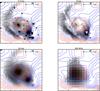 |
Fig. 8 12CO(3−2) contours overlaid onto the IRAC emissions at 3.6 μm (top left panel) and 8 μm (top right panel), at 24 μm from MIPS (bottom left panel), and at 843 MHz from SUMSS (bottom right panel). The molecular cavity is indicated by the central red contours. |
3.4. Cold-dust distribution
The continuum emission in the far-IR allowed us to investigate the distribution of the cold dust in the region. In the left panel of Fig. 7, we display the distribution of the emission at 870 μm, while in the right panel we show an overlay of this emission (in grayscale) and the 12CO emission (in contours) in the region observed in molecular lines, which is indicated with a red square in the left panel. The different symbols mark the position of candidate YSOs.
The image on the left shows dust cores centered at RA, Dec(J2000) = (10h38m00s, –58°46′45′′) (hereafter called D1), RA, Dec(J2000) = (10h37m54s, –58°46′15′′) (D2), RA, Dec(J2000) = (10h38m10s, –58°45′33′′) (D3), and RA, Dec(J2000) = (10h38m05s, –58°45′10′′) (D4). The last two cores appear to be embedded in extended emission. An additional core is detected at RA, Dec(J2000) = (10h37m51s, –58°47′18′′), much farther out of the region observed in molecular lines. The image on the right reveals the remarkable correspondence between the cold-dust emission at 870 μm and the CO emission. In particular, core D1 coincides with the densest section of the molecular shell, seen in the C18O image, and the extended dust emission to the west of the IRAS position agrees with the western section of the molecular shell. Moreover, the central cavity detected in CO lines is also present in the distribution of the continuum emission as a low-emission region. These facts confirm the presence of a cold-dust counterpart to the molecular shell. Finally, there is an excellent correspondence between the emission at 870 μm and the Herschel emission at 350 μm shown by Ohlendorf et al. (2013).
Source 4 is projected onto the border of the extended cold-dust emission. Sources 5 and 6 coincide with D1, while source 2 appears to be projected onto its border. Additionally, J103810.2-584527 and J103807.2-584511 (indicated by diamonds), mentioned by Ohlendorf et al. (2013), are projected onto the borders of D3 and D4. The coincidence of these sources with both molecular gas and cold dust is compatible with their identification as YSOs.
4. Discussion
4.1. Comparison with infrared and radio continuum emissions
Figure 8 shows an overlay of the 12CO contours of Fig. 6 and the emissions at 3.6 μm from IRAC, 8 μm from IRAC, 24 μm from MIPS, and 843 MHz from SUMSS.
In the 3.6 μm image we can see a number of point-like sources spread across the surveyed region, which were identified as belonging to a cluster by Ohlendorf et al. (2013). Source 3 (class II) from Table 3 is projected near the center of the cavity detected in CO lines, and source 2 (class II) appears to be close to the border of the cavity. Sources 4, 5 and 6, classified as class I objects, are projected onto the dense molecular envelope. The arc-like structure mentioned by Ohlendorf et al. (2013) is seen in coincidence with the denser regions of the molecular shell.
The emission at 8 μm arises mainly from both the polycyclic aromatic hydrocarbons (PAHs, Leger & Puget 1984) and from an underlying continuum emission attributed to very small grains, and is typical of photodissociation regions (PDRs). These molecules cannot survive inside Hii regions. They delineate the interface between ionized and molecular gas, indicating a clear interaction between them. Weak 8 μm emission partially coincident with the central cavity is probably located at this interface. The arc-like feature identified at 3.6 μm is also detected at 8 μm and at 5.8 μm (not shown here and also mainly originating from PAH emission), and, as shown by Ohlendorf et al. (2013), can be identified in the MIPS emission at 24 μm and in the Herschel image at 70 μm (see Fig. 12 from Ohlendorf et al. 2013). This arc-like feature appears to be projected onto the bright CO emission regions, which indicates regions where photodissociation of the molecular gas occurs.
The 24 μm emission arises from warm dust. In addition to a diffuse extended emission coincident with the cavity, the image shows that sources 2 and 3 (class II) are the brighter sources in the mid-IR.
The continuum image at 843 MHz indicates the presence of radio emission within the shell. The origin of this emission is probably thermal and due to ionized gas, since it spatially coincides with emission at 24 μm caused by warm dust. The observed full width at half-maximum of the source at 843 GHz is 45″ × 62″. The mean diameter of this source, after deconvolution with the synthesized beam of the telescope (HPBW = 43″ × 43″ cosec(δ)), is ≤25′′. The source is centered at RA, Dec(J2000) = (10h38m053, –58°46′2709), coincident within errors with the position of source 3, suggesting the existence of ionized gas within the cavity and in the close environs of this source. A radio continuum image at higher frequency than 843 MHz with better angular resolution would be useful to investigate the ionized gas distribution within the cavity and to determine its physical parameters, since thermal emission is optically thick below 1 GHz.
The emission distribution at 8 and 24 μm, and in the radio continuum toward this region resembles that seen toward many infrared dust bubbles identified by Churchwell et al. (2006; see Watson et al. 2009), and is indicative of the action of UV photons and stellar winds in the environs of excitation sources. These bubbles also appear to be encircled by molecular gas (see, for example, Zhang et al. 2013).
Parameters of the molecular shell.
4.2. Physical parameters of the molecular gas and dust
As described in previous sections, our APEX data obtained with medium angular resolution revealed a molecular shell within clump 6 from the list of Yonekura et al. (2005; see Fig. 1). In what follows we estimate its main physical parameters, which are summarized in Table 4.
We defined Δvtotal as the velocity range where the shell can be identified. It was estimated as Δvtotal = vi − vf, where vi and vf are the initial and final velocities at which the molecular emission is clearly detected in connection to this shell. These values were estimated from Fig. 5 as vi = −20.8 and vf = −25.3 km s-1.
The radius of the cavity rcav was estimated by taking into account the contour corresponding to Tmb−12 = 17 K as the inner radius of the envelope in the left panel of Fig. 6. The result is given in arcseconds and pc. The outer radius of the envelope rmax was measured following the outer contour of 17 K. Finally, the radius of the shell rshell was estimated as a mean value between rcav and rmax.
The mean column density of 13CO, N13CO, in the observed region was calculated assuming LTE, using the equations of Rohlfs & Wilson (2004) and the image in the middle panel of Fig. 6. For the 13CO(3−2) we obtain ![Mathematical equation: \begin{equation} \left[\frac{N_{\rm 13CO}}{\rm cm^{-2}}\right] = C T_{\rm exc} \int \tau^{13}(\nu){\rm d}\nu \left[ \frac{{\rm e}^{\frac{2h\nu}{kT_{\rm exc}}}}{{\rm e}^{\frac{h \nu}{k T_{\rm exc}}}-1} \right], \label{eq:N13} \end{equation}](/articles/aa/full_html/2014/10/aa23369-14/aa23369-14-eq106.png) (4)where
(4)where  (5)Folowing Rohlfs & Wilson (2004), we can approximate
  (6)As pointed out by Rohlfs & Wilson (2004), this expression helps to eliminate to some extend optical-depth effects. We adopted the optical depth of the 13CO(3−2) line corresponding to the most intense velocity component (see Table 2). Finally, the average H2 column density NH2 = 1.1 × 1022 cm-2 was obtained by adopting NH2 = 7.7 × 10⁵N13CO (Wilson & Rood 1994).
To calculate the total molecular mass MH2 in the observed region we applied ![Mathematical equation: \begin{equation} \left[\frac{M_{\rm H_{2}}}{M_{\odot}}\right] = C' \left[\frac{N_{\rm H_{2}}}{\rm cm^{-2}}\right] \left[\frac{\rm Area}{\arcsec}\right] \left[\frac{d^{2}}{\rm kpc}\right], \label{eq:masa} \end{equation}](/articles/aa/full_html/2014/10/aa23369-14/aa23369-14-eq112.png) (7)where the constant C′ = 5.17 × 10⁻²⁵ includes the value of the solar mass 2×1033 g, the mean molecular weight μ = 2.76, derived after allowance of a relative helium abundance of 25% by mass (Allen 1973), and the hydrogen atomic mass mH = 1.67 × 10⁻²⁴ g. In this expression Area is the area of the molecular emission within a region of 90″ × 90″ in, and d = 2.5 ± 0.5 kpc. We obtained MH2 = 290 ± 110 M⊙. This value includes all the gas in the line of sight toward the observed region, which is ~10−15% of the total area of the clump.
(7)where the constant C′ = 5.17 × 10⁻²⁵ includes the value of the solar mass 2×1033 g, the mean molecular weight μ = 2.76, derived after allowance of a relative helium abundance of 25% by mass (Allen 1973), and the hydrogen atomic mass mH = 1.67 × 10⁻²⁴ g. In this expression Area is the area of the molecular emission within a region of 90″ × 90″ in, and d = 2.5 ± 0.5 kpc. We obtained MH2 = 290 ± 110 M⊙. This value includes all the gas in the line of sight toward the observed region, which is ~10−15% of the total area of the clump.
Derived parameters of the far- IR cores (870 μm).
Then, we derived the ambient density nH2 in the clump as  (8)We distributed the total molecular mass within the volume of a box of cross-section equal to that of the observed area (l2 with l = 90″ = 1.1 pc), and a size of
  or 2.9 pc (L) in the line of sight, which corresponds to the size of clump 6 in the line of sight equal to its minor axis, as evaluated in Fig. 1.
We estimated nH2 ~ 1200 cm-3. This value is compatible with the ambient density obtained by Yonekura et al. (2005; 1600 cm-3) based on C18O(1−0) line data.
A rough estimate of the mass in the shell can be derived from the image in the middle panel of Fig. 6. Adopting the contour line corresponding to  K as the border of the central cavity and using the same equations as Rohlfs & Wilson (2004), we estimate a molecular mass of 40 ± 8 M⊙. The volume density in the shell, nH2−shell, was estimated by distributing the molecular mass within the volume of a ring with inner and outer radii rcav and rmax. This value is 2300 cm-3.
Following Bohlin et al. (1977), the visual absorption in the observed region can be estimated assuming that gas and dust are well mixed from  (9)By neglecting the Hi column density NHI and adopting NH2 = 1.1 × 1022 cm-2, a visual absorption Av = 9 mag is derived, compatible with Av-values estimated by Preibisch et al. (2014).
From the LABOCA data, we determine the dust emission at 870 μm I870 and estimate the H2 column density toward the (sub)mm cores (see Fig. 7) using  (10)where I870 = S870/ Ωbeam, Ωbeam is the beam solid angle, κ870 = 1.0 cm-2 g-1 is the dust opacity per unit mass estimated for dust grains with thin ice mantles in cold clumps (Ossenkopf & Henning 1994), and Rd is the adopted dust-to-gas ratio (=1/100). The core total mass (gas + dust mass) can be obtained from
  (11)Equations (10) and (11) where obtained from Miettinen & Harju (2010).
Table 5 summarizes the main parameters of the dust cores. Columns 1 to 3 identify the core and its coordinates, Col. 4 lists the flux density at 870 μm, Cols. 5 and 6 the total column density and mass. Column 7 gives the effective radius of the core, and Col. 8 the H2 volume density. Derived densities are roughly compatible with the H2 densities estimated from the molecular data. Note, however, that molecular data are available only for D1.
4.3. Proposed scenario
The presence of ionized gas, warm dust, and an extended PDR along with the high density derived for the region point toward the existence of an Hii region, in agreement with the classification of source 3 as a CHII region.
In this context, we propose that the Hii region originated in the photodissociation and ionization of part of the dense molecular clump. This interpretation is compatible with the observed decrease in intensity of the component at −22.8 km s-1 in the inner section of the shell, and the fact that the only component detected in HCO+ coincides with the CO component at −22.8 km s-1, which represents the bulk of the molecular gas in the clump.
It might be that the molecular shell is expanding. Hii regions expand in their vicinity owing to the difference in pressure between the ionized gas and the neutral gas that surrounds it. The difference between the H2 ambient volume density nH2 (~1200 cm-3) and the volume density in the shell nH2−shell (~2300 cm-3) suggests that the ionized region has started its expansion phase. However, an inspection of the position-velocity 12CO maps toward the cavity does not show clear signs of expansion. Moreover, bearing in mind an uncertainty of 20% in distance, errors in derived volume densities may be as high as 140%, and the difference between the two volume densities should be taken with caution. A scenario compatible with our findings suggests that the Hii region is young, close to the end of its formation phase, and/or just starting its expansion phase (see Dyson & Williams 1998).
We have investigated the presence of exciting sources within the cavity using the 2MASS catalog and taking into account sources with excellent photometric quality (AAA). The analysis of the sources was performed in a region of 20′′ in radius centered at RA, Dec(J2000) =(10h38m04s,–58°46′20′′). The color–color (CC) (H − Ks, J − H)- and color magnitude (CM) (H − Ks,Ks)-diagrams (the CC diagram is not shown here) revealed that 2MASS 10380461-5846233, coincident with MSX G286.3773-00.2563, is a candidate O9V star (H − Ks = 0.246, J − H = 0.505). The position of this source in the CM-diagram is indicated in Fig. 9, along with those of the other two AAA-sources found in the region. The 2MASS source 10380616-5846183 is a candidate B star, while 10380371-5846118, would be a later-B star.
Ohlendorf et al. (2013) estimated for 2MASS 10380461-5846233 a stellar mass of ~5.8 M⊙ from a spectral energy distribution obtained using the tool of Robitaille et al. (2007), which is not compatible with an O9V star. However, their result should be taken with caution since the fitting tool has some limitations (Deharveng et al. 2012; Robitaille 2008; Offner et al. 2012).
An Hii region developed within the cavity would have electron densities ne ≃ 2nH2 ≃ 2.4 × 103 cm-3, taking into account that the original material is molecular hydrogen. These electron densities, along with the small radius of the cavity, are roughly compatible with the presence of a compact Hii region (r ≤ 0.25 pc and ne ≥ 5 × 103 cm-3, Kurtz 2005). The diagram of Fig. 10 shows the UV flux NL vs. nH2. The curves indicate the UV photon flux necessary to ionize an Hii region as a function of the H2 ambient density nH2 = ne/2 for Strömgren radii of 0.22, 0.32 and 0.42 pc (corresponding to rcav, rshell and rmax). The horizontal line marks the UV flux corresponding to an O9V-type star (see Martins et al. 2002). According to the diagram, the UV flux NL of an O9V star would be enough to create an Hii region of 0.22 pc in size with a density of ~1.2× 103 cm-3.
We can also speculate that the presence of stellar winds can modify this picture. Stellar winds sweep up the surrounding material and create low-density cavities encircled by expanding shells (Weaver et al. 1977). Thus, the stellar wind from the O9V star may sweep up part of the ionized gas, thus decreasing the density of the Hii region and favoring the formation of an Hii region of 0.22−0.32 pc in radius. Additional studies are necessary to test this possibility.
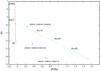 |
Fig. 9 CM diagram for the AAA-sources within the cavity. Absolute magnitudes for the ZAMS in the Ks band were obtained from Koornneef (1983). The green dashed line shows the reddening vector. |
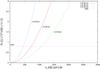 |
Fig. 10 UV photon flux NL vs. H2 ambient density. The curves indicate the UV flux NL as function of nH2 corresponding to different Strömgren radii. The horizontal line shows the theoretical UV flux for an O9V-type star (Smith et al. 2002). |
5. Summary
Based on 12CO, 13CO, C18O, HCO+, and CS line observations and millimeter continuum at 870 μm obtained with the APEX telescope, we analyzed the spatial distribution and the main physical parameters of the molecular gas and the cold dust associated with a dense clump linked to IRAS 10361-5830, located in the environs of the Hii region Gum 31 at 2.5±0.5 kpc.
The study allowed us to identify a molecular shell in the dense clump centered on the IRAS position. The analysis of the molecular emission reveals the existence of two velocity components projected onto the central cavity: a faint component centered at –25 km s-1 and a bright one centered at –22.8 km s-1, while generally only the bright velocity component appears to be projected onto the molecular shell. These velocities coincide with those of the material linked to Gum 31. The cold dust counterpart of the molecular shell is detected at 870 μm, as well as in Herschel data at 350 μm.
A comparison of the spatial distribution of the molecular shell with the emission at 24 μm revealed warm dust inside the molecular shell, suggesting the existence of ionizing sources, while the radio continuum image at 843 MHz showed diffuse emission coincident with the central molecular cavity and MSX G286.3773-00.2563. The Spitzer-IRAC emission at 8 μm showed an arc-like structure, also detected at 3.6, 5.8, and 24 μm, coincident with the densest region in the shell, suggesting the existence of a PDR at the interface between the ionized and molecular material.
The molecular shell has a mean radius of 0.32 pc and is detected within a velocity interval of 6.3 km s-1. We estimated a molecular mass in the shell of 40 ± 8 M⊙.
A number of candidate YSOs classified as class I and II objects appear to be projected onto the central cavity and the molecular shell. The presence of candidate YSOs indicates that star formation is active in this dense clump. The 2MASS source 10380461-5846233 (MSX G286.3773-00.2563), a candidate late O-type star, seems to be responsible for creating a compact Hii region inside the molecular clump.
Acknowledgments
We acknowledge the anonymous referee for useful comments. This project was partially financed by CONICET of Argentina under projects PIP 02488 and PIP 00356, and UNLP under project 11/G120. M.R. is supported by CONICYT of Chile through grant No. 1080335. This publication is based on data acquired with the Atacama Pathfinder Experiment (APEX). APEX is a collaboration between the Max-Planck-Institut fur Radioastronomie, the European Southern Observatory, and the Onsala Space Observatory. This research has made use of the NASA/ IPAC Infrared Science Archive, which is operated by the Jet Propulsion Laboratory, California Institute of Technology, under contract with the National Aeronautics and Space Administration. This work is based [in part] on observations made with the Spitzer Space Telescope, which is operated by the Jet Propulsion Laboratory, California Institute of Technology under a contract with NASA. This publication makes use of data products from the Two Micron All Sky Survey, which is a joint project of the University of Massachusetts and the Infrared Processing and Analysis Center/California Institute of Technology, funded by the National Aeronautics and Space Administration and the National Science Foundation. The MSX mission is sponsored by the Ballistic Missile Defense Organization (BMDO).
References
- Allen, C. W. 1973, Astrophysical quantities, 3rd edn. (London: University of London, Athlone Press) [Google Scholar]
- Barnes, P. J., Yonekura, Y., Fukui, Y., et al. 2011, ApJS, 196, 12 [NASA ADS] [CrossRef] [Google Scholar]
- Beltrán, M. T., Brand, J., Cesaroni, R., et al. 2006, A&A, 447, 221 [NASA ADS] [CrossRef] [EDP Sciences] [MathSciNet] [Google Scholar]
- Benjamin, R. A., Churchwell, E., Babler, B. L., et al. 2003, PASP, 115, 953 [NASA ADS] [CrossRef] [Google Scholar]
- Bohlin, R. C., Savage, B. D., & Drake, J. F. 1977, NASA STI/Recon Technical Report N, 78, 13984 [NASA ADS] [Google Scholar]
- Cappa, C., Niemela, V. S., Amorín, R., & Vasquez, J. 2008, A&A, 477, 173 (CNAV08) [NASA ADS] [CrossRef] [EDP Sciences] [Google Scholar]
- Carey, S. J., Noriega-Crespo, A., Mizuno, D. R., et al. 2009, PASP, 121, 76 [NASA ADS] [CrossRef] [Google Scholar]
- Churchwell, E., Povich, M. S., Allen, D., et al. 2006, ApJ, 649, 759 [NASA ADS] [CrossRef] [Google Scholar]
- Dedes, C., Leurini, S., Wyrowski, F., et al. 2011, A&A, 526, A59 [NASA ADS] [CrossRef] [EDP Sciences] [Google Scholar]
- Deharveng, L., Zavagno, A., Anderson, L. D., et al. 2012, A&A, 546, A74 [NASA ADS] [CrossRef] [EDP Sciences] [Google Scholar]
- Dionatos, O., Nisini, B., Cabrit, S., Kristensen, L., & Pineau Des Forêts, G. 2010, A&A, 521, A7 [NASA ADS] [CrossRef] [EDP Sciences] [Google Scholar]
- Dutra, C. M., Bica, E., Soares, J., & Barbuy, B. 2003, A&A, 400, 533 [NASA ADS] [CrossRef] [EDP Sciences] [Google Scholar]
- Elmegreen, B. G., & Lada, C. J. 1977, ApJ, 214, 725 [NASA ADS] [CrossRef] [Google Scholar]
- Koornneef, J. 1983, A&A, 128, 84 [NASA ADS] [Google Scholar]
- Kurtz, S. 2005, in Massive Star Birth: A Crossroads of Astrophysics, eds. R. Cesaroni, M. Felli, E. Churchwell, & M. Walmsley, IAU Symp., 227, 111 [Google Scholar]
- Langer, W. D., & Penzias, A. A. 1990, ApJ, 357, 477 [NASA ADS] [CrossRef] [Google Scholar]
- Leger, A., & Puget, J. L. 1984, A&A, 137, L5 [NASA ADS] [Google Scholar]
- Martins, F., Schaerer, D., & Hillier, D. J. 2002, A&A, 382, 999 [NASA ADS] [CrossRef] [EDP Sciences] [Google Scholar]
- Mauch, T., Murphy, T., Buttery, H. J., et al. 2003, MNRAS, 342, 1117 [NASA ADS] [CrossRef] [Google Scholar]
- Miettinen, O., & Harju, J. 2010, A&A, 520, A102 [NASA ADS] [CrossRef] [EDP Sciences] [Google Scholar]
- Offner, S. S. R., Robitaille, T. P., Hansen, C. E., McKee, C. F., & Klein, R. I. 2012, ApJ, 753, 98 [NASA ADS] [CrossRef] [Google Scholar]
- Ohlendorf, H., Preibisch, T., Gaczkowski, B., et al. 2013, A&A, 552, A14 [NASA ADS] [CrossRef] [EDP Sciences] [Google Scholar]
- Ossenkopf, V., & Henning, T. 1994, A&A, 291, 943 [NASA ADS] [Google Scholar]
- Preibisch, T., Mehlhorn, M., Townsley, L., Broos, P., & Ratzka, T. 2014, A&A, 564, A120 [NASA ADS] [CrossRef] [EDP Sciences] [Google Scholar]
- Robitaille, T. P. 2008, in Massive Star Formation: Observations Confront Theory, eds. H. Beuther, H. Linz, & T. Henning, ASP Conf. Ser., 387, 290 [Google Scholar]
- Robitaille, T. P., Whitney, B. A., Indebetouw, R., & Wood, K. 2007, ApJS, 169, 328 [NASA ADS] [CrossRef] [Google Scholar]
- Rohlfs, K., & Wilson, T. L. 2004, Tools of radio astronomy, 4th rev. and enl. edn. (Berlin: Springer) [Google Scholar]
- Sánchez-Monge, Á., Palau, A., Estalella, R., Beltrán, M. T., & Girart, J. M. 2008, A&A, 485, 497 [NASA ADS] [CrossRef] [EDP Sciences] [Google Scholar]
- Siringo, G., Kreysa, E., Kovács, A., et al. 2009, A&A, 497, 945 [NASA ADS] [CrossRef] [EDP Sciences] [Google Scholar]
- Smith, L. J., Norris, R. P. F., & Crowther, P. A. 2002, MNRAS, 337, 1309 [NASA ADS] [CrossRef] [Google Scholar]
- Vassilev, V., Meledin, D., Lapkin, I., et al. 2008, A&A, 490, 1157 [NASA ADS] [CrossRef] [EDP Sciences] [Google Scholar]
- Watson, C., Corn, T., Churchwell, E. B., et al. 2009, ApJ, 694, 546 [NASA ADS] [CrossRef] [Google Scholar]
- Weaver, R., McCray, R., Castor, J., Shapiro, P., & Moore, R. 1977, ApJ, 218, 377 [NASA ADS] [CrossRef] [Google Scholar]
- Wilson, T. L., & Rood, R. 1994, ARA&A, 32, 191 [NASA ADS] [CrossRef] [Google Scholar]
- Yonekura, Y., Asayama, S., Kimura, K., et al. 2005, ApJ, 634, 476 [NASA ADS] [CrossRef] [Google Scholar]
- Zhang, C.-P., Wang, J.-J., & Xu, J.-L. 2013, A&A, 550, A117 [NASA ADS] [CrossRef] [EDP Sciences] [Google Scholar]
All Tables
All Figures
|
Fig. 1 12CO(1−0) line emission distribution toward clump number 6 from the list of Yonekura et al. (2005), in RA, Dec(J2000) coordinates, extracted from CNAV08. Contour lines go from 4.0 to 8.0 K in steps of 1 K. The 4.0 K contour delineates approximately the clump as defined in C18O. The grayscale goes from 0 to 10 K. The large square indicates the region observed in molecular lines with APEX (see Sect. 2.1). The triangle indicates the position of IRAS 10361-5530. The different symbols mark the location of candidate YSOs identified by CNAV08 and Ohlendorf et al. (2013): MSX sources (circles), 2MASS sources (crosses), Herschel sources (diamonds), and WISE sources (plus signs). |
| In the text | |
|
Fig. 2 13CO(3−2) profiles observed in a 1.́5 × 1.́5 region around IRAS 10361-5830. Each profile shows Tmb in the interval from –1 to 25 K vs. LSR velocity in the range from –30 to –15 km s-1. The (0, 0) position coincides with the position of the IRAS source in J2000 equatorial coordinates. |
| In the text | |
|
Fig. 3 12CO(3−2), 13CO(3−2), and C18O(3−2) averaged profiles in black lines. Gaussian fittings are overlaid in red and blue lines. The sum of the Gaussian components in each profile is shown in green. |
| In the text | |
|
Fig. 4 13CO(3−2) spectrum (red) overlaid on the HCO+(4−3) spectrum (black) observed toward IRAS 10361-5830. The inset shows the HCO+ spectrum at an appropriate scale. |
| In the text | |
|
Fig. 5 Series of 12CO images showing the emission in the range –27.1 to –19.9 km s-1. The velocity of each panel is shown in the top-left corner of each panel. Contours go from 10 to 60 K in steps of 2 K. The central cross on each panel indicates the position of IRAS 10631-5830. The grayscale is indicated. Note that in this figure, RA increases toward the right. |
| In the text | |
|
Fig. 6 Left panel: average 12CO line emission Tmb−12 within the velocity interval from –27.1 to –19.9 km s-1. Contours go from 14 to 24 K, in steps of 1 K. Middle panel: average image of the 13CO line emission showing Tmb−13 within the velocity interval from –27.1 to –20.8 km s-1. Contours go from 3 to 10 K in steps of 0.5 K. Right panel: average image of the C18O line emission showing Tmb−18 within the velocity interval from –25.0 to –21.1 km s-1. Contours are 0.51, 0.68, 0.85, 1.02, 1.19, 1.70, 2.04, and 2.38 K. The triangle indicates the position of IRAS 10361-5530. The different symbols mark the location of candidate YSOs identified by CNAV08 and Ohlendorf et al. (2013): MSX sources (circles) and WISE sources (plus signs). White contours in the left panel correspond to Tmb ≤ 17 K. |
| In the text | |
|
Fig. 7 Left panel: 870 μm continuum emission map. Dust clumps are indicated. The grayscale goes from −0.1 to 2.0 Jy beam-1. Contour levels correspond to 0.2, 0.35, 0.5, and 0.7 Jy beam-1, and from 0.75 to 2.0 Jy beam-1 in steps of 0.25 Jy beam-1. The large square indicates the region observed in CO lines and the different symbols have the same meaning as in Fig. 6. Right panel: overlay of the emission at 870 μm (grayscale) and the CO contours of Fig. 6. IR sources listed in Table 3 are indicated. |
| In the text | |
|
Fig. 8 12CO(3−2) contours overlaid onto the IRAC emissions at 3.6 μm (top left panel) and 8 μm (top right panel), at 24 μm from MIPS (bottom left panel), and at 843 MHz from SUMSS (bottom right panel). The molecular cavity is indicated by the central red contours. |
| In the text | |
|
Fig. 9 CM diagram for the AAA-sources within the cavity. Absolute magnitudes for the ZAMS in the Ks band were obtained from Koornneef (1983). The green dashed line shows the reddening vector. |
| In the text | |
|
Fig. 10 UV photon flux NL vs. H2 ambient density. The curves indicate the UV flux NL as function of nH2 corresponding to different Strömgren radii. The horizontal line shows the theoretical UV flux for an O9V-type star (Smith et al. 2002). |
| In the text | |
Current usage metrics show cumulative count of Article Views (full-text article views including HTML views, PDF and ePub downloads, according to the available data) and Abstracts Views on Vision4Press platform.
Data correspond to usage on the plateform after 2015. The current usage metrics is available 48-96 hours after online publication and is updated daily on week days.
Initial download of the metrics may take a while.