| Issue |
A&A
Volume 569, September 2014
|
|
|---|---|---|
| Article Number | A65 | |
| Number of page(s) | 11 | |
| Section | Planets and planetary systems | |
| DOI | https://doi.org/10.1051/0004-6361/201424266 | |
| Published online | 24 September 2014 | |
Detecting the spin-orbit misalignment of the super-Earth 55 Cancri e⋆
1 Institut d’astrophysique de Paris,
UMR 7095 CNRS, Université Pierre & Marie Curie, 98bis boulevard Arago, 75014
Paris,
France
e-mail: This email address is being protected from spambots. You need JavaScript enabled to view it.
2 Observatoire de Haute-Provence,
CNRS/OAMP, 04870
Saint-Michel-l’Observatoire,
France
Received:
24
May
2014
Accepted:
25
June
2014
Abstract
We present time-resolved spectroscopy of transits of the super-Earth 55 Cnc e using HARPS-N observations. We devised an empirical correction for the “color effect” on the radial velocity residuals from the Keplerian fit, which significantly improves their dispersion with respect to the HARPS-N pipeline standard data reduction. Using our correction, we were able to detect the smallest Rossiter-McLaughlin anomaly amplitude of an exoplanet so far (~60 cm/s). The super-Earth 55 Cnc e is also the smallest exoplanet with a Rossiter-McLaughlin anomaly detection. We measured the sky-projected obliquity λ = 72.4-11.5+12.7°, indicating that the planet orbit is prograde, highly misaligned and nearly polar compared to the stellar equator. The entire 55 Cancri system may have been highly tilted by the presence of a stellar companion.
Key words: Planets and satellites: dynamical evolution and stability / techniques: radial velocities / stars: individual: 55 Cancri
Table 4 is available in electronic form at http://www.aanda.org
© ESO, 2014
1. Introduction
Spectroscopic observations during the transit of an exoplanet across its host star can measure the sky-projected angle between the spins of the planetary orbit and the stellar rotation (namely the obliquity) through the Rossiter-McLaughlin (RM) effect (Holt 1893; Rossiter 1924; McLaughlin 1924). The occultation of a rotating star by a planet distorts the apparent stellar line shape by removing the profile part emitted by the hidden portion of the star. This induces anomalous stellar radial velocity variations during the transit, which constrain the sky-projected obliquity (λ). Whereas first observed systems revealed aligned, prograde orbits (e.g., Queloz et al. 2000; Winn et al. 2005; Loeillet et al. 2008), first misaligned systems were reported with the cases of XO-3 (Hébrard et al. 2008; Winn et al. 2009c; Hirano et al. 2011) and HD 80606 (Moutou et al. 2009; Pont et al. 2009; Winn et al. 2009a; Hébrard et al. 2010). About thirty misaligned systems have been identified today over more than eighty measured systems1 (Albrecht et al. 2012; Crida & Batygin 2014), including some with retrograde or nearly polar orbits (e.g., Winn et al. 2009b; Narita et al. 2010; Triaud et al. 2010; Hébrard et al. 2011). These unexpected results favor scenarios where close-in massive planets have been brought in by planet-planet (or planet-star) scattering, Kozai migration, and/or tidal friction, rather than more standard scenarios implying disk migration that are expected to conserve the initial alignment between the angular momentums of the disk and of the planetary orbits (see, e.g., Fabrycky & Tremaine 2007; Guillochon et al. 2011), although some models show that the initial misalignment of a planet can be maintained through its interactions with the disk (Teyssandier et al. 2013). Alternatively, it has been proposed that the orbit still reflects the orientation of the disk, with the stellar spin instead having moved away, either early-on through magnetosphere-disk interactions (Lai et al. 2011) or later through elliptical tidal instability (Cébron et al. 2011).
Log of the HARPS-N observations.
Obliquity measurements have mainly been done in single-planet systems, mostly on hot-Jupiters. In recent years, they have been extended to transiting multiplanet systems, most of which host super-Earths. Obliquities have been derived from the RM anomaly in the systems KOI-94 (Hirano et al. 2012; Albrecht et al. 2013) and Kepler-25 (Albrecht et al. 2013), from starspot variations of Kepler-30 (Sanchis-Ojeda et al. 2012), and from the measure of the stellar inclination via asteroseismology in the sytems Kepler-50 and Kepler-65 (Chaplin et al. 2013), and the system Kepler-410 (Van Eylen et al. 2014). These systems have shown coplanar orbits that are well aligned with the stellar equator, hinting that their orbital planes still trace the primordial alignment of the protoplanetary disk responsible for the planets’ migrations, while the apparent isotropic distribution of obliquities of hot-Jupiters is the result of dynamical interactions (Albrecht et al. 2013). This conclusion has recently been put in doubt by the large obliquity of the two-planet system Kepler-56 (Huber et al. 2013) and the possible spin-orbit misalignements of several multicandidate Kepler systems (Walkowicz & Basri 2013; Hirano et al. 2014).
The exoplanet 55 Cnc e offers the opportunity to probe spin-orbit misalignments in the domains of both multiple systems and super-Earths. It is part of a five-planet system, which was first detected and characterized with radial velocity measurements (Fischer et al. 2008). The orbital period of the closest and lightest of them, planet 55 Cnc e, was a subject of debate because of the aliasing in the radial velocity datasets. The value P = 0.7365 days proposed by Dawson & Fabrycky (2010) was confirmed when Winn et al. (2011) with MOST and Demory et al. (2011) with Warm Spitzer, detected photometric transits of planet e at the ephemeris corresponding to that short period. Subsequent studies have refined the orbital and transit parameters of 55 Cnc e using additional photometry and radial velocity measurements (e.g., Demory et al. 2012; Gillon et al. 2012; Endl et al. 2012). Thus, 55 Cnc e is an unusually close-in (a = 0.015 au) super-Earth with a mass Mp = 7.99 ± 0.25 M⊕ (Nelson et al. 2014) and a radius Rp = 1.99 ± 0.08 R⊕ in the optical (Dragomir et al. 2014).
55 Cnc is the only naked-eye star hosting a transiting planet. The brightness of that nearby G8V star (V = 5.95, d = 12.3 pc) makes it a particularly advantageous target for follow-up studies. In particular, it allowed the brightness temperature measurement of 55 Cnc e (T = 2360 ± 300 K) thanks to Spitzer observation of occultations (Demory et al. 2012), as well as the possible detection of H i in the atmosphere of 55 Cnc b (P = 14.652 days, Mp = 7.8 ± 0.6 M⊕) with HST (Ehrenreich et al. 2012), indicating that this planet might host an extended atmosphere and suggesting that the orbits of all the planets of the system are nearly coplanar. The orbital evolution of this closely packed system has motivated several studies that also point toward a coplanar and dynamically stable system (Nelson et al. 2014; Kaib et al. 2011; Boué & Fabrycky 2014). Kaib et al. (2011) show that the 55 Cnc system should be highly misaligned with a true obliquity of ~65°, while Boué & Fabrycky (2014) point out that this requires the stellar spin axis to be weakly coupled to the planets’ orbits. Although the detection of the RM anomaly of planet e is expected to be challenging (amplitude <1 m/s), its short period, small radius, and its part in a complex multiple system makes it a particularly interesting target for investigating misalignment.
We describe in Sect. 2 the observations made with the HARPS-N spectrograph. In Sect. 3 we describe the color effect and its correction, in Sect. 4 we present the detection of the Rossiter-McLaughlin anomaly, and in Sect. 5 we test its robustness. Discussion of the results will be found in Sect. 6.
2. Observations and data reduction
We obtained time to observe a total of eight different transits of 55 Cnc e over three different semesters between late 2012 and early 2014 with the spectrograph HARPS-N at the 3.58-m Telescopio Nazionale Galileo (TNG, La Palma, Spain). HARPS-N is a fiber-fed, cross-dispersed, environmentally stabilized echelle spectrograph dedicated to high-precision radial velocity measurements (Cosentino et al. 2012). It provides the resolution power λ/ Δλ = 115 000. The light is dispersed on 69 spectral orders from 383 to 690 nm. Due to weather and technical problems, three of the eight scheduled transits could not be observed at all. The log of the five observed transits (runs hereafter labeled from A to E) is reported in Table 1. Runs A to D were executed in service mode by the TNG Team, whereas Run E was made in visiting mode by us.
All the observations were sequences of about thirty successive exposures of six-minute durations each. We chose that duration as a compromise between accuracy, temporal resolution, and overheads. Each sequence lasts several hours (about three hours typically, whereas the full transit lasts 1.5 h). For technical reasons, a poor coverage of the transit was obtained during Run A, with only six measurements secured during the transit itself. The four other runs allowed good coverage of the whole transit duration to be obtained. Reference observations were secured immediately before and after the transit for Runs B, D, and E; for Runs A and C, those reference observations were secured mainly after the transit. The observations of Run E had to be stopped earlier than scheduled due to a sudden degradation of the weather conditions after the end of the transit.
The CCD was used in its fast readout mode with a speed of 500 kHz. We used the two 1′′-wide optical-fiber apertures: the first one was on the target, whereas the second one was used for simultaneous radial-velocity reference, using the thorium-argon lamp or the Fabry Perot depending of the run (see Table 1). The two first exposures of Run A are an exception, since they were observed without simultaneous reference, the second aperture being on the nearby sky.
Owing to different weather conditions (seeing and absorption), the signal-to-noise ratios (S/Ns) were different among the five runs. Table 1 reports typical S/Ns for each run in three different parts of the spectra: Runs C and D were obtained in poor conditions and provide data of relatively low accuracy, Runs B and E were obtained in good conditions and provide particularly high-accuracy data, whereas Run A is intermediate.
The S/N values reported in Table 1 are the median among the ~30 exposures of a given run in a given spectral order. In fact, the S/N is varying significantly with time during a given run, and these variations are of different amplitudes from one spectral order to the other. This means that there is a global variation in the flux during a run, but also a variation in the distribution of the flux with the color (hereafter named “color effect”). The global and chromatic S/N variations show random structures on different time scales, which are probably mainly due to short-term variations in the weather conditions. They also show regular, lower-frequency variations that could be explained by the airmass change of the target during each run, which translates into wavelength-dependent throughput variations. The airmass evolution during each run is reported in Table 1. The airmass monotonously varies for all the runs but the first one. In the case of Run A, the target reached the meridian during the sequence; it implied an interruption of the observations after the first seven exposures, then a change in the orientation of the alt-azimuth TNG telescope before starting the observations again. The few radial velocities obtained during transit A were thus secured in different conditions than the reference ones obtained after that transit. Runs B to E were fully executed after the target reached the meridian.
The HARPS-N spectra were extracted from the detector images with the DRS pipeline, which includes localization of the spectral orders on the 2D-images, optimal order extraction, cosmic-ray rejection, corrections of flat-field, wavelength calibration with thorium-argon lamp exposures made during the afternoon, and short-term radial-velocity drift correction from simultaneous references with thorium-argon or Fabry Perot. Then the spectra passed through weighted cross-correlation with a G2-type numerical masks following the method described by Baranne et al. (1996) and Pepe et al. (2002). All the exposures provide a well-defined, single peak in the cross-correlation function (CCF), whose Gaussian fits allow the radial velocities to be measured, together with their associated uncertainties. We tested different kinds of numerical masks as well as removing some low-S/N spectral orders from the cross-correlation; this did not significantly change the observed radial velocity variations. All these procedures were made for Run A using the version 3.6 of the HARPS-N DRS pipeline, which did not include any correction of the color effect. The DRS version 3.7, which includes a correction of the color effect, was available in 2014 and we used it for the data of Runs B to E.
3. Empirical correction of the color effect on the radial velocities
The radial velocities of 55 Cnc were fitted with a Keplerian model taking the five planets of the system into account. For each run the fit was performed on the measurements outside of the transit of planet e, assumed to be on a circular orbit. Its transit epoch, transit duration, and period were taken from Dragomir et al. (2014), and the semi-amplitude of its radial velocity variations from Endl et al. (2012). Parameters for the other planets were also taken from Endl et al. (2012).
We observed a trend over each entire run in the radial velocity residuals from the Keplerian fit (see example for Run A in Fig. 1), which we interpret as being due to the color effect (Sect. 2). The CCF represents a mean profile of the thousands of stellar lines in the 69 HARPS-N spectral orders, whose Gaussian fit provides the radial velocity measurement. Because the flux color balance between the spectra varies during a run, this affects the relative contribution of each spectral order to the mean Doppler shift of the CCF, and thus the measured radial velocity.
To characterize and quantify the chromatic variations, we defined a “color ratio” between the S/Ns associated to the 69 spectral orders: 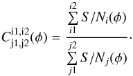 (1)where S/Nk(φ) represents the S/N of spectral order k (k varying from 0 to 68, following the DRS pipeline orders numbering) at orbital phase φ. The S/Ns at the numerator are summed between spectral orders i1 and i2 (included), and the S/Ns at the denominator are summed between j1 and j2. We looked for the combination of spectral orders that gives the best correlation between the color ratio and the RV residuals to the Keplerian fit. For each combination we fitted the data outside of the transit with a polynomial regression, using the Bayesian information criterion (BIC) to prevent over-fitting with a high-order polynomial (Crossfield et al. 2012; Cowan et al. 2012). For each run we found a good correlation between the variations in the color ratio and those of the residuals to the Keplerian fit. As an example, Fig. 1 shows the similarities between the variations in these two quantities in the case of Run A, as well as their linear correlation. This allows us to apply an empirical correction of the color effect to the radial velocities, which improves their adjustment to the Keplerian curve (see, e.g., Run A in Fig. 2). The correlation is also shown in Fig. 3 in the case of Run E. As explained below, this run has the best transit observation.
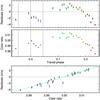 |
Fig. 1 Top: residuals from the Keplerian fit in Dataset A as a function of
orbital phase. Vertical dashed lines show the times of mid-transit, first, and fourth
contacts. The colors of the plotted circles indicate the orbital phases of each
observation. Middle: color ratio
|

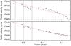 |
Fig. 2 Top: radial velocity measurements without any color-effect correction (black points) and their Keplerian fit (dashed red line) during Run A. Vertical dashed lines show the times of mid-transit, first, and fourth contacts. Bottom: after the empirical color-effect correction, radial velocity measurements outside of the transit are well-adjusted to the Keplerian fit, improving the out-of transit dispersion from 1.92 m/s to 0.23 m/s. |
Best parameters for the empirical correction of the color effect in each run.
Runs B to E include a DRS standard color-effect correction that was not available for Run A (see Sect. 2). We could thus apply our empirical correction on Datasets B to E, extracted without the DRS standard color-effect correction, and compare the two different methods. Table 2 shows the dispersions of the residuals to the Keplerian fit outside of the transit for both color-effect corrections. The dispersion is always smaller in the case of our empirical correction, in some cases decreasing by more than a factor 2. With the present observations of 55 Cnc e, the empirical correction thus appears to give a better correction of the color effect than the DRS standard correction (Fig. 4 shows Dataset E reduced with both methods), and we adopt it hereafter.
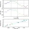 |
Fig. 3 Same plot as in Fig. 1 for Dataset E. Again, there is a linear correlation between the RV residuals and a color ratio, in this case |
We show in Table 2 the best-fit parameters for the empirical correction of each dataset. The best correlation between color ratio and RV residuals is always linear, except for Run B, which requires a third-order polynomial correction. Although this dataset has a high precision, it is apparently affected by additional systematics and shows oscillations with an amplitude up to several dm/s. We did not find any correlation between these oscillations and the color effect or any other parameter, and their origin is unclear. Datasets C and D have low S/Ns and still show a large, uncorrelated dispersion after correction. The last measurement of Dataset D had to be excluded to find an acceptable correlation between color ratio and RV residuals. Dataset A was obtained in different conditions than the other datasets, in particular with data during the transit secured in different conditions than the reference ones outside the transit (see Sect. 2). Run E thus provides the best dataset, with a good sampling and a dispersion of the RV residuals after our empirical correction that is improved to the level where the Rossiter-McLaughlin anomaly can be detected for a super-Earth such as 55 Cnc e (Fig. 4). For these reasons, we first fit the Rossiter-McLaughlin anomaly in Dataset E only (Sect. 4) and then analyze the influence of the other datasets (Sect. 5).
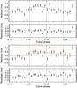 |
Fig. 4 Upper panels: residuals from the Keplerian fit in Dataset E (black diamonds), after the empirical color-effect correction; (top). The dispersion outside the transit is 28 cm/s. The solid red line shows the best fit of the Rossiter-McLaughlin anomaly with |


Parameters for the Rossiter-McLaughlin analysis of 55 Cnc e.
4. Detection of the Rossiter-McLaughlin anomaly and obliquity measurement
After applying the empirical color-effect correction, radial velocities of Dataset E were fitted in order to derive the sky-projected angle λ between the planetary orbital axis and the stellar rotation axis. We applied the analytical approach developed by Ohta et al. (2005) to model the form of the Rossiter-McLaughlin anomaly, which is described by ten parameters: the stellar limb-darkening linear coefficient ϵ, the transit parameters Rp/R∗, ap/R∗, and ip, the parameters of the circular orbit (P, T0, and K), the systemic radial velocity γ, the projected stellar rotation velocity vsini∗, and λ. We adopted a linear limb-darkening correction with ϵ = 0.648 (Dragomir et al. 2014). Parameters for the Keplerian fit are the same as in Sect. 3, and the additional transit parameters for planet e were taken from Dragomir et al. (2014; see Table 3).
We computed the χ2 of the fit on a grid scanning all possible values for λ, vsini∗, and γ. Once the minimum χ2 and corresponding best values for these parameters were obtained, we calculated their error bars from an analysis of the χ2 variation; that is, a given parameter is pegged at various trial values, and for each trial value we run an extra fit, allowing all the other parameters to vary freely. The 1σ error bars for the pegged parameter are then obtained when its value yields a χ2 increase of 1 from the minimum (see, e.g., Hébrard et al. 2002). We detected the RM anomaly with  ° and vsini∗ = 3.3 ± 0.6 km s-1 (Fig. 4). The best fit provides a reduced χ2 of 2.2; to be conservative, we increased the error bars on the radial velocity measurements by a factor
  to obtain a reduced χ2 of 1. As a result, we adopt λ = 72.4
 and vsini∗ = 3.3 ± 0.9 km s-1. The derived vsini∗ agrees with the value 2.5±0.5 km s-1 obtained by Valenti & Fischer (2005). The systemic radial velocity γ was determined with a particularly high precision of ±8 cm/s; however, it depends on the correlation mask, the spectral orders, and the color correction, so the actual barycentric stellar radial velocity is not as accurate. The dispersion of the residuals for the best fit (28 cm/s) is similar to the estimated out-of-transit dispersion (Table 2). Results are summarized in Table 3.
We performed an F-test to evaluate the significance of the RM anomaly detection (see, e.g., Hébrard et al. 2011). We note that in our case the errors may not be normally distributed and independent, and thus the F-test is done as a rough estimate. Including the RM model in the fit improves the χ2 over the 27 measurements secured during Run E from 95.8 to 51.8, for two additional free parameters (λ and vsini∗). The statistical test indicates there is a probability >90% that the χ2 improvement is due to the RM anomaly detected. We thus conclude that we detected the RM anomaly of 55 Cnc e with  . Its orbit is prograde and highly misaligned, the planet transiting mainly the blueshifted regions of the stellar disk (Fig. 5).
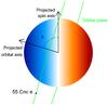 |
Fig. 5 View of 55 Cnc along the line of sight. With the star rotation, the light emitted by the half of the stellar disk moving toward the observer is blueshifted, while the light from the other half that moves away is redshifted. During the transit, the small super-Earth 55 Cnc e (shown as a black disk, to scale) mainly transits the blueshifted half of the stellar disk because of its high sky-projected obliquity λ = 72.4°. |
5. Validation tests
Because of the small radius of the super-Earth 55 Cnc e and the low rotation velocity of its star, the detection of its RM anomaly is challenging. In addition, we applied a new empirical method for correcting the color effect. Thus in this section we check the robustness of the detection of 55 Cnc e RM anomaly presented in Sect. 4. To be conservative, all error bars on the free model parameters hereafter are scaled and enlarged to maintain a reduced χ2 of 1.
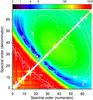 |
Fig. 6 Dependence of the RM anomaly fit on the spectral orders used to compute the color-effect correction (Run E). Two different spectral orders must be used to quantify the color, which explains the white diagonal line where no fits can be done. White contours show the spin-orbit angles obtained for each color ratio (solid lines for positive values, dashed lines for negative values). The colorscale corresponds to the χ2 difference with respect to the best fit, obtained with the spectral orders 21 and 28 (white disk) and λ = 72.4°. Color ratios in the red part of the diagram show no significant correlation between the residuals of the Keplerian fit and the color ratio. Fits at less than about 3σ from the best fit are found in the localized blue area. |
5.1. Analysis of Run E
In a first time we performed five kinds of tests on Dataset E alone.
-
Fitting technique Minimizing the χ2 or the out-of-transit dispersion of the residuals, instead of the BIC, gives the same values for the spectral orders used in the empirical color-effect correction provided the polynomial degree is fixed to prevent overfitting. Calculating the RM model by resampling each six-minute exposure by ten (e.g., Kipping 2010) has no influence on our results. This was expected because the modeled radial velocity variations during the exposure times are smaller than the error bars (see Fig. 4).
-
Ephemeris The empirical color-effect correction is based on measurements outside of the 55 Cnc e transit, to prevent removing its RM anomaly unintentionally. Thus we investigated how our results depend on 55 Cnc e ephemeris, i.e., the mid-transit T0, the period P, and the transit duration tdur. We quadratically propagated the errors on the mid-transit time taking the number of revolutions accomplished by 55 Cnc e between T0 and Run E transit epoch into account. Because we do not have enough measurements to constrain the transit mid-time and the period with high accuracy, we had to choose between the values derived by Dragomir et al. (2014); Gillon et al. (2012). We decided to adopt the values obtained by the former because they used long-time baseline MOST photometry of the 55 Cnc sytem, with data obtained in 2012 in addition to the 2011 MOST data used by Gillon et al. (2012). This reduces the uncertainties on the mid-transit times of our runs, based on their measurement of T0, and provides a higher precision value for the orbital period and planet to star radii ratio of 55 Cnc e. Nonetheless, we also performed the RM anomaly fit using the ephemeris of Gillon et al. (2012). In this case T0(E), the mid-transit time of Run E, is about 11 min later, and the transit duration about 8 min shorter, than with Dragomir et al. (2014). Three measurements switch between inside/outside the transit, and the color correction is thus different. We obtained
 km s-1, and
  ° at 3σ from the previous estimation in Sect. 4. It must be noted that the fit is of lower
quality, with a reduced χ2 of 3.6 and a dispersion of the
residuals to the RM fit of 36 cm/s (instead of χ2 = 2.2
and a dispersion of 28 cm/s). Nonetheless we again detect the RM anomaly with a
highly misaligned orbit, nearly polar. We varied T0(E) within its
1σ
error bars using the ephemeris measured by Dragomir
et al. (2014). Because of the large number of revolutions (1065)
accomplished by 55 Cnc e since the measure of T0, the
uncertainty on T0(E) is about
5.5 min, roughly twice that of T0. We also increased the transit
duration by its upper 1σ error bar (~5 min). We found that using
lower values for T0(E) has no
significant impact on our results, whereas with higher values there are not enough
measurements after the transit to properly correct for the color effect. This shows
that enough measurements must be taken both before and after the transit for the
color-effect correction to be efficient.
° at 3σ from the previous estimation in Sect. 4. It must be noted that the fit is of lower
quality, with a reduced χ2 of 3.6 and a dispersion of the
residuals to the RM fit of 36 cm/s (instead of χ2 = 2.2
and a dispersion of 28 cm/s). Nonetheless we again detect the RM anomaly with a
highly misaligned orbit, nearly polar. We varied T0(E) within its
1σ
error bars using the ephemeris measured by Dragomir
et al. (2014). Because of the large number of revolutions (1065)
accomplished by 55 Cnc e since the measure of T0, the
uncertainty on T0(E) is about
5.5 min, roughly twice that of T0. We also increased the transit
duration by its upper 1σ error bar (~5 min). We found that using
lower values for T0(E) has no
significant impact on our results, whereas with higher values there are not enough
measurements after the transit to properly correct for the color effect. This shows
that enough measurements must be taken both before and after the transit for the
color-effect correction to be efficient. -
Color-effect correction We fitted the RM anomaly to the data extracted with the DRS standard color-effect correction (Fig. 4). The anomaly is detected with vsini∗ = 2.9 ± 1.3 km s-1 and λ = 88.6
 °. This prograde, highly misaligned orbit is in good agreement
with the RM anomaly detected after the empirical color-effect correction, although
as expected the quality of the fit is lower with a reduced χ2 of 3.6
and a dispersion of the residuals to the RM fit of 39 cm/s. We investigated how our
results depend on the spectral orders used for the empirical color correction. We
fixed a linear correction and calculated the best-fit parameters of the RM anomaly
with all possible color ratios. To keep things simple, the color ratios are
calculated with only two spectral orders (i.e. i1 =
i2, j1 = j2). The results are
shown in Fig. 6. As expected, the diagram is
roughly symmetric, which shows that fits performed with a color ratio or its inverse
(e.g.,
°. This prograde, highly misaligned orbit is in good agreement
with the RM anomaly detected after the empirical color-effect correction, although
as expected the quality of the fit is lower with a reduced χ2 of 3.6
and a dispersion of the residuals to the RM fit of 39 cm/s. We investigated how our
results depend on the spectral orders used for the empirical color correction. We
fixed a linear correction and calculated the best-fit parameters of the RM anomaly
with all possible color ratios. To keep things simple, the color ratios are
calculated with only two spectral orders (i.e. i1 =
i2, j1 = j2). The results are
shown in Fig. 6. As expected, the diagram is
roughly symmetric, which shows that fits performed with a color ratio or its inverse
(e.g.,  and
and  ) have about the same quality and give similar
values for λ. For most ratios, λ is obtained with a
high value between 50 and 110° and stellar velocities between 0.5 and 5 km s-1. Only a specific range
of spectral orders provides an acceptable adjustment to the data, all with
λ-values around 70°. In this range, the best adjustments
are obtained with a short separation between the spectral orders at the numerator
and the denominator of the color ratio, as expected from our results for all
datasets in Table 2.
) have about the same quality and give similar
values for λ. For most ratios, λ is obtained with a
high value between 50 and 110° and stellar velocities between 0.5 and 5 km s-1. Only a specific range
of spectral orders provides an acceptable adjustment to the data, all with
λ-values around 70°. In this range, the best adjustments
are obtained with a short separation between the spectral orders at the numerator
and the denominator of the color ratio, as expected from our results for all
datasets in Table 2. -
Model parameters The derived values remained within their uncertainties when we varied the limb-darkening coefficient ϵ between 0.1 and 0.9. This was expected from the precision of our measurements during the ingress and egress. Increasing the eccentricity of the orbit up of 0.06 (e.g., Demory et al. 2012) and using other values for the semi-amplitude of planet e (e.g., Nelson et al. 2014) does not change the shape of the Keplerian fit significantly during and around the transit, and has thus little infuence on our results. The same is true for the parameters of the outer planets. Varying Rp/R∗ and ap/R∗ within their small 1σ error bars has no significant influence on our results. We used the values of Dragomir et al. (2014) for these two parameters, since the radius in particular is measured in the optical bandpass of MOST and is more appropriate to our analysis based on HARPS-N data than the radius measured in the infrared with Spitzer (Gillon et al. 2012). We noted that the obliquity is sensitive to the inclination. While the quality of the fit remains unchanged, varying the inclination ip between the 1σ error bars obtained by Dragomir et al. (2014) results in uncertainties of +10.3/−7.2° for λ. These uncertainties are calculated as the differences between the best-fit values in Sect. 4 and those obtained while varying ip. They are similar to the uncertainties derived in Sect. 4.
-
Convective blueshift Because of the small amplitude of the measured RM anomaly (~60 cm/s), our interpretation of the radial velocity measurements may also be sensitive to the impact of the convective blueshift (CB) effect. We included the calculation of the CB radial velocity blueshift in our model, following the prescription of Shporer & Brown (2011). Assuming a solar value for the local convective blueshift (−300 m/s) and a linear limb-darkening law, we found that the CB effect has little influence on our results, with a maximum amplitude of about 4 cm/s at the center of the transit which is well below the error bars on the radial velocity measurements. Since the distortion due to the CB effect increases with higher orbital inclinations, we performed the fit again while varying ip between its 1σ error bars. Even then, results were similar to those obtained when varying ip without CB effect, the derived uncertainties varying by less than 1° for λ and 0.1 km s-1 for vsini∗). We also note that 55 Cnc is a G8 star, and thus its local convective blueshift is likely lower than for the Sun.
 . We caution that the value of vsini∗ may not be well
constrained by our data, although this has no impact on the obliquity. While the analytic
formula derived by Ohta et al. (2005) has been
known to underestimate the velocity anomaly (e.g., Triaud
et al. 2009; Hirano et al. 2010), it
provides a good approximation when the stellar spin velocity is low enough. Increasing our
best-fit value for vsini∗ by 10% (i.e.,
the systematic error in the case of HD 209458b, which rotates faster than 55 Cnc; Winn et al. 2005) was found to have no influence on the
inferred obliquity. The value of 2.5 ±
0.5 km s-1 obtained by Valenti
& Fischer (2005) may actually be a hint that our value for vsini∗ is overestimated.
Assuming vsini∗ =
2 km s-1, we
obtained an obliquity of 62°
which remains within the derived uncertainties. Smaller vsini∗ values do not
provide a good fit to the data, considering that the RM anomaly is detected with a
significant amplitude.
. We caution that the value of vsini∗ may not be well
constrained by our data, although this has no impact on the obliquity. While the analytic
formula derived by Ohta et al. (2005) has been
known to underestimate the velocity anomaly (e.g., Triaud
et al. 2009; Hirano et al. 2010), it
provides a good approximation when the stellar spin velocity is low enough. Increasing our
best-fit value for vsini∗ by 10% (i.e.,
the systematic error in the case of HD 209458b, which rotates faster than 55 Cnc; Winn et al. 2005) was found to have no influence on the
inferred obliquity. The value of 2.5 ±
0.5 km s-1 obtained by Valenti
& Fischer (2005) may actually be a hint that our value for vsini∗ is overestimated.
Assuming vsini∗ =
2 km s-1, we
obtained an obliquity of 62°
which remains within the derived uncertainties. Smaller vsini∗ values do not
provide a good fit to the data, considering that the RM anomaly is detected with a
significant amplitude.
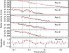 |
Fig. 7 Best model of the RM anomaly when fitting Datasets A to E simultaneously. Black points show radial velocity measurements as a function of the orbital phase (see Table 4), overlaid with the five-planet Keplerian fit ignoring the transit (dashed, red line), and the final fit including the model of the RM anomaly (solid, red line). Vertical dotted lines show the times of mid-transit, first, and fourth contacts. The simultaneous fit to the five runs provides similar results to the fit to Run E alone. The bottom panel shows the error-weighted average of the Keplerian residuals over all runs (residuals from the Keplerian fit are first calculated in each run and grouped in common phase bins of width 0.01). Although the combined residuals are dominated by systematic errors, the RM anomaly is clearly visible. |
5.2. Analysis of all runs
Although Runs A to D have lower qualities than Run E (Sect. 3), we checked their consistency with the RM anomaly detected on Dataset E. First we fit all datasets simultaneously, taking into account the five planets of the system in the Keplerian model. The radial velocity measurements after correction of the color effect are reported in Table 4 and displayed in Fig. 7. The error-weighted average of the Keplerian residuals over all runs clearly shows the RM anomaly detection despite the systematic errors (lower panel in Fig. 7). The results are within 1σ of those obtained with Dataset E only with λ = 68.3 ± 6.6°, but the dispersion of the RV residuals to the RM fit is much higher (71 cm/s). We obtained similar results when fitting all runs simultaneously except Run E, with λ = 65.2 ± 8.4° and a dispersion of 77 cm/s.
Second we attempted to fit each dataset independently. Run A poorly samples the transit and was observed in two different modes; in addition the data secured during the transit were obtained in a different configuration than the reference data obtained after the transit. This makes Run A suspicious for the RM study, and indeed the fit did not succeed. As mentioned previously (Sect. 3), Run B shows radial velocity oscillations of unclear origin. This may be due to the presence of starspots or granulation on the stellar surface (e.g., Boisse et al. 2011; Dumusque et al. 2011) or an instrumental effect. Despite these perturbations, the empirical color-effect correction allows detecting the RM anomaly with λ = 77.1 ± 7.3° but a larger dispersion of the residuals than in Run E (54 cm/s instead of 28 cm/s). We obtain similar results with Dataset C, although the presence of an outlier at orbital phase 0 results in an abnormally high value for vsini∗. Removing this outlier, we obtain λ = 65.9 ± 15.2° and a dispersion of 72 cm/s. Finally we performed an F-test for the RM anomaly in Run D in the same way as in Sect. 4, and found a 50% false positive probability due to the high noise in this dataset, indicating that the anomaly is likely not detected in this run.
We conclude that given their lower quality, Datasets A to D agrees with the RM anomaly detected in Run E.
6. Discussion
We report the detection of the Rossiter-McLaughlin anomaly of the super-Earth 55 Cnc e, with a sky-projected obliquity  . The planet is on a prograde and highly misaligned orbit, nearly polar. This detection is mainly based on one high-accuracy transit observed with HARPS-N, and thus more observations of the same quality as Run E are needed to confirm the detection. The super-Earth 55 Cnc e is the smallest exoplanet for which the projected spin-orbit alignment has been measured2, and is also the planet with the smallest RM anomaly amplitude detected (~0.6 m/s) below the Neptune-like exoplanet HAT-P-11 b (1.5 m/s; Winn et al. 2010b) and Venus (1 m/s; Molaro et al. 2013). We were able to detect the RM anomaly by devising an empirical color-effect correction for the chromatic variations known to affect radial velocity measurements. This correction is based on the S/Ns associated to HARPS-N spectral orders, and it may prove a useful tool for improving the accuracy of RV measurements from other stars or instruments. Indeed in the present study our empirical correction was found to improve the dispersion of the RV measurements with respect to the standard DRS correction, and with observing sequences of a few hours we detected the RM anomaly of 55 Cnc e with high accuracy (<30 cm/s).
The 55 Cnc system is well approximated by a coplanar system (Kaib et al. 2011; Ehrenreich et al.
2012; Nelson et al. 2014), and thus all its
planets are likely highly misaligned with the stellar spin axis. While most multiplanet
systems have been found aligned with the stellar equator, this is the second occurrence of a
highly misaligned one after Kepler-56 (Huber et al.
2013). This is a hint that large obliquities are not restricted to isolated
hot-Jupiters as a consequence of a dynamical migration scenario. The high obliquity of 55
Cnc e agrees with lower mass planets being either prograde and aligned, or strongly
misaligned (Hébrard et al. 2010, 2011), although that trend was mainly seen on isolated,
Jupiter-mass planets. It is also a new exception to the apparent trend that misaligned
planets tend to orbit hot stars (Winn et al. 2010a;
the effective temperature of 55 Cnc derived by von Braun et
al. 2011 is Teff = 5196 K). That tidal interactions
did not align the system (Barker & Ogilvie 2009)
during its long lifetime (10.2 Gy; von Braun et al.
2011) may be due to the low mass of its star, the low mass of its closest companion
55 Cnc e, and the complex dynamical interactions within this compact multiple system (Nelson et al. 2014). The particularity of the 55 Cnc and
Kepler-56 systems may be the presence of a wide-orbit companion. Although such companions
may be present in other multiple systems, none have been detected. If the companion is
initially inclined with respect to the protoplanetary disk, or with the inner planets around
the primary star, it may misalign their orbital planes while preserving their coplanarity
(e.g., Batygin 2012; Kaib et al. 2011). Kaib et al. (2011)
investigated this scenario in the case of the 55 Cnc system, whose stellar companion 55 Cnc
B was detected at a projected distance of 1065 AU (Mugrauer
et al. 2006). With a semi-major axis lower than about 4000 au the gravitational
influence of 55 Cnc B is strong enough to significantly alter the alignment of the system,
provided the star is on a highly eccentric orbit (e ≳ 0.95; Boué & Fabrycky
2014). Kaib et al. (2011) predict a true
obliquity of ~65°,
which is remarkably consistent with the sky-projected obliquity of 72.4 we derived, and indicate that the rotation axis of 55 Cnc
A is probably not inclined much toward the line of sight.
Online material
Online material
The Holt-Rossiter-McLaughlin Encyclopaedia: http://www.physics.mcmaster.ca/~rheller/
Stellar obliquities have been measured for the host stars of three smaller planets (Kepler-50b, 1.71 R⊕; Kepler-65b, 1.42 R⊕; Kepler-65d, 1.52 R⊕) using asteroseismology (Chaplin et al. 2013), but this technique does not provide a direct measurement of the projected spin-orbit angle.
Acknowledgments
We deeply thank the referee T. Hirano for his thoughtful comments. We would also like to thank J.-M. Almenara, F. Bouchy, M. Deleuil, R. F. Díaz, A. Lecavelier des Étangs, G. Montagnier, C. Moutou, and A. Santerne for their help and advice. This publication is based on observations collected with the the HARPS-N spectrograph on the 3.58-m Italian Telescopio Nazionale Galileo (TNG) operated on the island of La Palma by the Fundación Galileo Galilei of the INAF (Instituto Nazionale di Astrofisica) at the Spanish Observatorio del Roque de los Muchachos of the Instituto de Astrofisica de Canarias (programs OPT12B_13, OPT13B_30, and OPT14A_34 from OPTICON common time allocation process for EC supported trans-national access to European telescopes). We thank the TNG staff for support. The authors acknowledge the support of the French Agence Nationale de la Recherche (ANR), under program ANR-12-BS05-0012 “Exo-Atmos”.
References
- Albrecht, S., Winn, J. N., Johnson, J. A., et al. 2012, ApJ, 757, 18 [NASA ADS] [CrossRef] [Google Scholar]
- Albrecht, S., Winn, J. N., Marcy, G. W., et al. 2013, ApJ, 771, 11 [NASA ADS] [CrossRef] [Google Scholar]
- Baranne, A., Queloz, D., Mayor, M., et al. 1996, A&AS, 119, 373 [NASA ADS] [CrossRef] [EDP Sciences] [Google Scholar]
- Barker, A. J., & Ogilvie, G. I. 2009, MNRAS, 395, 2268 [NASA ADS] [CrossRef] [Google Scholar]
- Batygin, K. 2012, Nature, 491, 418 [NASA ADS] [CrossRef] [PubMed] [Google Scholar]
- Boisse, I., Bouchy, F., Hébrard, G., et al. 2011, A&A, 528, A4 [NASA ADS] [CrossRef] [EDP Sciences] [Google Scholar]
- Boué, G., & Fabrycky, D. C. 2014, ApJ, 789, 111 [NASA ADS] [CrossRef] [Google Scholar]
- Cébron, D., Moutou, C., Le Bars, M., Le Gal, P., & Fares, R. 2011 [arXiv:1101.4531] [Google Scholar]
- Chaplin, W. J., Sanchis-Ojeda, R., Campante, T. L., et al. 2013, ApJ, 766, 101 [NASA ADS] [CrossRef] [Google Scholar]
- Cosentino, R., Lovis, C., Pepe, F., et al. 2012, in SPIE Conf. Ser., 8446 [Google Scholar]
- Cowan, N. B., Machalek, P., Croll, B., et al. 2012, ApJ, 747, 82 [NASA ADS] [CrossRef] [Google Scholar]
- Crida, A., & Batygin, K. 2014, A&A, 567, A42 [NASA ADS] [CrossRef] [EDP Sciences] [Google Scholar]
- Crossfield, I. J. M., Knutson, H., Fortney, J., et al. 2012, ApJ, 752, 81 [NASA ADS] [CrossRef] [Google Scholar]
- Dawson, R. I., & Fabrycky, D. C. 2010, ApJ, 722, 937 [NASA ADS] [CrossRef] [Google Scholar]
- Demory, B.-O., Gillon, M., Deming, D., et al. 2011, A&A, 533, A114 [NASA ADS] [CrossRef] [EDP Sciences] [Google Scholar]
- Demory, B.-O., Gillon, M., Seager, S., et al. 2012, ApJ, 751, L28 [Google Scholar]
- Dragomir, D., Matthews, J. M., Winn, J. N., & Rowe, J. F. 2014, in IAU Symp. 293, ed. N. Haghighipour, 52 [Google Scholar]
- Dumusque, X., Santos, N. C., Udry, S., Lovis, C., & Bonfils, X. 2011, A&A, 527, A82 [NASA ADS] [CrossRef] [EDP Sciences] [Google Scholar]
- Ehrenreich, D., Bourrier, V., Bonfils, X., et al. 2012, A&A, 547, A18 [NASA ADS] [CrossRef] [EDP Sciences] [Google Scholar]
- Endl, M., Robertson, P., Cochran, W. D., et al. 2012, ApJ, 759, 19 [NASA ADS] [CrossRef] [Google Scholar]
- Fabrycky, D., & Tremaine, S. 2007, ApJ, 669, 1298 [NASA ADS] [CrossRef] [Google Scholar]
- Fischer, D. A., Marcy, G. W., Butler, R. P., et al. 2008, ApJ, 675, 790 [NASA ADS] [CrossRef] [Google Scholar]
- Gillon, M., Demory, B.-O., Benneke, B., et al. 2012, A&A, 539, A28 [NASA ADS] [CrossRef] [EDP Sciences] [Google Scholar]
- Guillochon, J., Ramirez-Ruiz, E., & Lin, D. 2011, ApJ, 732, 74 [NASA ADS] [CrossRef] [Google Scholar]
- Hébrard, G., Lemoine, M., Vidal-Madjar, A., et al. 2002, ApJS, 140, 103 [NASA ADS] [CrossRef] [Google Scholar]
- Hébrard, G., Bouchy, F., Pont, F., et al. 2008, A&A, 488, 763 [NASA ADS] [CrossRef] [EDP Sciences] [Google Scholar]
- Hébrard, G., Désert, J.-M., Díaz, R. F., et al. 2010, A&A, 516, A95 [NASA ADS] [CrossRef] [EDP Sciences] [Google Scholar]
- Hébrard, G., Ehrenreich, D., Bouchy, F., et al. 2011, A&A, 527, L11 [NASA ADS] [CrossRef] [EDP Sciences] [Google Scholar]
- Hirano, T., Suto, Y., Taruya, A., et al. 2010, ApJ, 709, 458 [NASA ADS] [CrossRef] [Google Scholar]
- Hirano, T., Narita, N., Sato, B., et al. 2011, PASJ, 63, L57 [NASA ADS] [Google Scholar]
- Hirano, T., Narita, N., Sato, B., et al. 2012, ApJ, 759, L36 [NASA ADS] [CrossRef] [Google Scholar]
- Hirano, T., Sanchis-Ojeda, R., Takeda, Y., et al. 2014, ApJ, 783, 9 [NASA ADS] [CrossRef] [Google Scholar]
- Holt, J. R. 1893, A&A, 12, 646 [Google Scholar]
- Huber, D., Carter, J. A., Barbieri, M., et al. 2013, Science, 342, 331 [NASA ADS] [CrossRef] [PubMed] [Google Scholar]
- Kaib, N. A., Raymond, S. N., & Duncan, M. J. 2011, ApJ, 742, L24 [NASA ADS] [CrossRef] [Google Scholar]
- Kipping, D. M. 2010, MNRAS, 408, 1758 [NASA ADS] [CrossRef] [Google Scholar]
- Lai, D., Foucart, F., & Lin, D. N. C. 2011, MNRAS, 412, 2790 [NASA ADS] [CrossRef] [Google Scholar]
- Loeillet, B., Shporer, A., Bouchy, F., et al. 2008, A&A, 481, 529 [NASA ADS] [CrossRef] [EDP Sciences] [Google Scholar]
- McLaughlin, D. B. 1924, ApJ, 60, 22 [NASA ADS] [CrossRef] [Google Scholar]
- Molaro, P., Monaco, L., Barbieri, M., & Zaggia, S. 2013, MNRAS, 429, L79 [NASA ADS] [CrossRef] [Google Scholar]
- Moutou, C., Hébrard, G., Bouchy, F., et al. 2009, A&A, 498, L5 [NASA ADS] [CrossRef] [EDP Sciences] [Google Scholar]
- Mugrauer, M., Neuhäuser, R., Mazeh, T., et al. 2006, Astron. Nachr., 327, 321 [NASA ADS] [CrossRef] [Google Scholar]
- Narita, N., Hirano, T., Sanchis-Ojeda, R., et al. 2010, PASJ, 62, L61 [NASA ADS] [Google Scholar]
- Nelson, B. E., Ford, E. B., Wright, J. T., et al. 2014, MNRAS [arXiv:1402.6343] [Google Scholar]
- Ohta, Y., Taruya, A., & Suto, Y. 2005, ApJ, 622, 1118 [NASA ADS] [CrossRef] [Google Scholar]
- Pepe, F., Mayor, M., Galland, F., et al. 2002, A&A, 388, 632 [NASA ADS] [CrossRef] [EDP Sciences] [Google Scholar]
- Pont, F., Hébrard, G., Irwin, J. M., et al. 2009, A&A, 502, 695 [NASA ADS] [CrossRef] [EDP Sciences] [Google Scholar]
- Queloz, D., Eggenberger, A., Mayor, M., et al. 2000, A&A, 359, L13 [NASA ADS] [Google Scholar]
- Rossiter, R. A. 1924, ApJ, 60, 15 [NASA ADS] [CrossRef] [Google Scholar]
- Sanchis-Ojeda, R., Fabrycky, D. C., Winn, J. N., et al. 2012, Nature, 487, 449 [NASA ADS] [CrossRef] [PubMed] [Google Scholar]
- Shporer, A., & Brown, T. 2011, ApJ, 733, 30 [NASA ADS] [CrossRef] [Google Scholar]
- Teyssandier, J., Terquem, C., & Papaloizou, J. C. B. 2013, MNRAS, 428, 658 [NASA ADS] [CrossRef] [Google Scholar]
- Triaud, A. H. M. J., Queloz, D., Bouchy, F., et al. 2009, A&A, 506, 377 [NASA ADS] [CrossRef] [EDP Sciences] [Google Scholar]
- Triaud, A. H. M. J., Collier Cameron, A., Queloz, D., et al. 2010, A&A, 524, A25 [NASA ADS] [CrossRef] [EDP Sciences] [Google Scholar]
- Valenti, J. A., & Fischer, D. A. 2005, ApJS, 159, 141 [NASA ADS] [CrossRef] [MathSciNet] [Google Scholar]
- Van Eylen, V., Lund, M. N., Silva Aguirre, V., et al. 2014, ApJ, 782, 14 [NASA ADS] [CrossRef] [Google Scholar]
- von Braun, K., Boyajian, T. S., ten Brummelaar, T. A., et al. 2011, ApJ, 740, 49 [NASA ADS] [CrossRef] [Google Scholar]
- Walkowicz, L. M., & Basri, G. S. 2013, MNRAS, 436, 1883 [NASA ADS] [CrossRef] [Google Scholar]
- Winn, J. N., Noyes, R. W., Holman, M. J., et al. 2005, ApJ, 631, 1215 [NASA ADS] [CrossRef] [Google Scholar]
- Winn, J. N., Howard, A. W., Johnson, J. A., et al. 2009a, ApJ, 703, 2091 [NASA ADS] [CrossRef] [Google Scholar]
- Winn, J. N., Johnson, J. A., Albrecht, S., et al. 2009b, ApJ, 703, L99 [NASA ADS] [CrossRef] [Google Scholar]
- Winn, J. N., Johnson, J. A., Fabrycky, D., et al. 2009c, ApJ, 700, 302 [NASA ADS] [CrossRef] [Google Scholar]
- Winn, J. N., Fabrycky, D., Albrecht, S., & Johnson, J. A. 2010a, ApJ, 718, L145 [NASA ADS] [CrossRef] [Google Scholar]
- Winn, J. N., Johnson, J. A., Howard, A. W., et al. 2010b, ApJ, 723, L223 [NASA ADS] [CrossRef] [Google Scholar]
- Winn, J. N., Matthews, J. M., Dawson, R. I., et al. 2011, ApJ, 737, L18 [NASA ADS] [CrossRef] [Google Scholar]
All Tables
All Figures
|
Fig. 1 Top: residuals from the Keplerian fit in Dataset A as a function of
orbital phase. Vertical dashed lines show the times of mid-transit, first, and fourth
contacts. The colors of the plotted circles indicate the orbital phases of each
observation. Middle: color ratio
|
| In the text | |
|
Fig. 2 Top: radial velocity measurements without any color-effect correction (black points) and their Keplerian fit (dashed red line) during Run A. Vertical dashed lines show the times of mid-transit, first, and fourth contacts. Bottom: after the empirical color-effect correction, radial velocity measurements outside of the transit are well-adjusted to the Keplerian fit, improving the out-of transit dispersion from 1.92 m/s to 0.23 m/s. |
| In the text | |
|
Fig. 3 Same plot as in Fig. 1 for Dataset E. Again, there is a linear correlation between the RV residuals and a color ratio, in this case |
| In the text | |
|
Fig. 4 Upper panels: residuals from the Keplerian fit in Dataset E (black diamonds), after the empirical color-effect correction; (top). The dispersion outside the transit is 28 cm/s. The solid red line shows the best fit of the Rossiter-McLaughlin anomaly with |
| In the text | |
|
Fig. 5 View of 55 Cnc along the line of sight. With the star rotation, the light emitted by the half of the stellar disk moving toward the observer is blueshifted, while the light from the other half that moves away is redshifted. During the transit, the small super-Earth 55 Cnc e (shown as a black disk, to scale) mainly transits the blueshifted half of the stellar disk because of its high sky-projected obliquity λ = 72.4°. |
| In the text | |
|
Fig. 6 Dependence of the RM anomaly fit on the spectral orders used to compute the color-effect correction (Run E). Two different spectral orders must be used to quantify the color, which explains the white diagonal line where no fits can be done. White contours show the spin-orbit angles obtained for each color ratio (solid lines for positive values, dashed lines for negative values). The colorscale corresponds to the χ2 difference with respect to the best fit, obtained with the spectral orders 21 and 28 (white disk) and λ = 72.4°. Color ratios in the red part of the diagram show no significant correlation between the residuals of the Keplerian fit and the color ratio. Fits at less than about 3σ from the best fit are found in the localized blue area. |
| In the text | |
|
Fig. 7 Best model of the RM anomaly when fitting Datasets A to E simultaneously. Black points show radial velocity measurements as a function of the orbital phase (see Table 4), overlaid with the five-planet Keplerian fit ignoring the transit (dashed, red line), and the final fit including the model of the RM anomaly (solid, red line). Vertical dotted lines show the times of mid-transit, first, and fourth contacts. The simultaneous fit to the five runs provides similar results to the fit to Run E alone. The bottom panel shows the error-weighted average of the Keplerian residuals over all runs (residuals from the Keplerian fit are first calculated in each run and grouped in common phase bins of width 0.01). Although the combined residuals are dominated by systematic errors, the RM anomaly is clearly visible. |
| In the text | |
Current usage metrics show cumulative count of Article Views (full-text article views including HTML views, PDF and ePub downloads, according to the available data) and Abstracts Views on Vision4Press platform.
Data correspond to usage on the plateform after 2015. The current usage metrics is available 48-96 hours after online publication and is updated daily on week days.
Initial download of the metrics may take a while.