| Issue |
A&A
Volume 568, August 2014
|
|
|---|---|---|
| Article Number | A50 | |
| Number of page(s) | 12 | |
| Section | Interstellar and circumstellar matter | |
| DOI | https://doi.org/10.1051/0004-6361/201424036 | |
| Published online | 13 August 2014 | |
Cosmic ray induced ionisation of a molecular cloud shocked by the W28 supernova remnant
1 Univ. Grenoble Alpes/CNRS, IPAG, 38000 Grenoble, France
e-mail: This email address is being protected from spambots. You need JavaScript enabled to view it.
2 APC, AstroParticule et Cosmologie, Université Paris Diderot, CNRS, CEA, Observatoire de Paris, Sorbonne Paris, 75205 Paris, France
3 Institut d’Astrophysique de Paris, 98bis Bd Arago, 75014 Paris, France
Received: 19 April 2014
Accepted: 5 June 2014
Abstract
Cosmic rays are an essential ingredient in the evolution of the interstellar medium, as they dominate the ionisation of the dense molecular gas, where stars and planets form. However, since they are efficiently scattered by the galactic magnetic fields, many questions remain open, such as where exactly they are accelerated, what is their original energy spectrum, and how they propagate into molecular clouds. In this work we present new observations and discuss in detail a method that allows us to measure the cosmic ray ionisation rate towards the molecular clouds close to the W28 supernova remnant. To perform these measurements, we use CO, HCO+, and DCO+ millimetre line observations and compare them with the predictions of radiative transfer and chemical models away from thermodynamical equilibrium. The CO observations allow us to constrain the density, temperature, and column density towards each observed position, while the DCO+/HCO+ abundance ratios provide us with constraints on the electron fraction and, consequently, on the cosmic ray ionisation rate. Towards positions located close to the supernova remnant, we find cosmic ray ionisation rates much larger (≳100) than those in standard galactic clouds. Conversely, towards one position situated at a larger distance, we derive a standard cosmic ray ionisation rate. Overall, these observations support the hypothesis that the γ rays observed in the region have a hadronic origin. In addition, based on CR diffusion estimates, we find that the ionisation of the gas is likely due to 0.1−1 GeV cosmic rays. Finally, these observations are also in agreement with the global picture of cosmic ray diffusion, in which the low-energy tail of the cosmic ray population diffuses at smaller distances than the high-energy counterpart.
Key words: ISM: clouds / cosmic rays / ISM: supernova remnants / ISM: individual objects: W28
© ESO, 2014
1. Introduction
Cosmic rays (CRs) are energetic charged particles that reach the Earth as an isotropic flux. They pervade the Galaxy and play a crucial role in the evolution of the interstellar medium, because they dominate the ionisation of molecular clouds where the gas is shielded from the UV radiation field. The ionisation degree in the molecular gas is a fundamental parameter throughout the star and planet forming process. First, ions couple the gas to the magnetic field and, therefore, they regulate the gravitational collapse of the cloud. In addition, ions sustain turbulence within protoplanetary discs and introduce non-ideal magnetohydrodynamics effects, which influence the accretion rate onto the protostar (Balbus & Hawley 1998; Lesur et al. 2014). Finally, the CR induced ions initiate efficient chemical reactions in the cold molecular clouds, which eventually lead to the formation of complex molecules, which enrich the gas even up to the first stages of planet formation.
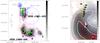 |
Fig. 1 Left: the W28 complex on large scales. Grayscale (in σ) and thick contours show TeV emission as seen by HESS (levels are 4−6σ). Red contours show the CO(1−0) emission (Dame et al. 2001) integrated over 15−25 km s-1 and magenta contours trace the emission integrated over 5−15 km s-1 (levels are 40−70 K km s-1 by 5 K km s-1). Crosses show the positions observed with the IRAM 30m telescope and discussed in this paper. The blue contours show the 20 cm free-free emission in the M20 region (Yusef-Zadeh et al. 2000). The blue circle gives the approximate radio boundary of the SNR W28 (Brogan et al. 2006). Right: the northern cloud in the W28 complex (zoom on the black box). The red contours show the CO(3−2) emission in K km s-1, integrated over 15−25 km s-1 (levels are 15−130 K km s-1 by 5 K km s-1) (Lefloch et al. 2008). Diamonds show the locations of OH masers in the region (Claussen et al. 1997). |
However, in order to fully understand the influence of CRs on the above processes across the Galaxy, it is necessary to know where CRs are accelerated and how they propagate through the gas. Unfortunately, since CRs are scattered by magnetic fields all along their path through the Galaxy, the production sites of CRs cannot be observed directly, and the diffusion of CRs also makes the evolution of the energy spectrum during their propagation difficult to determine observationally.
However, we can detect indirect signatures of the interaction of hadronic CRs (essentially protons) with matter. Protons above a kinetic energy threshold of ≈280 MeV produce π0 pions when they collide with particles in the molecular cloud. Each pion then decays into two γ-ray photons (π0 → 2γ), each with a typical energy that thoseis ~10% that of the colliding proton. Bright γ-ray sources thus indicate regions with a large density of protons with energies above 0.28 GeV. In these regions, the observed γ-ray photon spectrum can, in addition, be used to derive the spectrum of the parental CR particles, before the scattering and propagation within the Galaxy (Ackermann et al. 2013).
Supernova remnants (SNR) are thought to be the sources of CRs. In this scenario, protons are accelerated in the expanding shell of the SNR, following the diffusive shock acceleration process (Bell 1978). Supporting this scenario, there is now clear evidence that SNR are spatially associated with GeV to TeV sources (Aharonian 2013). Moreover, several SNR are close to the molecular cloud that gave birth to the SN precursor. These molecular clouds now act as reservoirs of target material for the freshly accelerated protons, thus enhancing the production rate of γ rays. Although it is compatible with γ-ray observations, the hadronic scenario is challenged by the leptonic scenario involving electron CRs. In this alternative scenario, the γ-ray emission can be explained mainly by inverse Compton scattering of the cosmic microwave background (e.g. Morlino et al. 2009; Abdo et al. 2011). Yet, this scenario cannot explain the spatial correlation of TeV emission with molecular clouds. Moreover, recent observations of the IC443 and W44 SNR with the Fermi-LAT telescope (Ackermann et al. 2013) specifically support a hadronic origin of γ rays, consistent with the so-called SNR paradigm for the origin of primary CR (see e.g. Hillas 2005,for a review).
Cosmic ray protons with kinetic energy below the ≈280 MeV threshold of π0 production cannot be traced by the emission of γ-rays. Nevertheless, recent calculations suggest that the ionisation of UV-shielded gas is mostly due to keV-GeV protons (Padovani et al. 2009). Accordingly, low-energy CR protons can be traced indirectly by measuring the ionisation fraction of the dense gas. It has thus been proposed that an enhanced electron abundance in molecular clouds located in the vicinity of SNR could be the smoking gun for the presence of freshly accelerated CRs, with energies ≲1 GeV.
This idea was put forward by Ceccarelli et al. (2011, hereafter CC2011), who measured the ionisation fraction xe = n(e−)/nH in the W51C molecular cloud, located in the vicinity of the W51 SNR. The detection of TeV emission by both HESS and MAGIC telescopes close to the molecular cloud is evidence of a physical interaction with the SNR. This supports the idea of the pion-decay production of γ rays with W51C acting as a γ-ray emitter. In CC2011, an enhanced ionisation fraction was reported towards one position, W51C-E, which required a CR ionisation rate two orders of magnitude larger than the typical value of 1 × 10-17 s-1 in molecular clouds. This observational evidence strongly supports the hadronic scenario of γ-ray production, at least for W51.
Complementary studies of the CR ionisation rate in several diffuse clouds close to SNR have been carried out using different techniques, such as  absorption (McCall et al. 2003). These studies also show an enhancement of a factor of 10−100 of the CR ionisation rate (Indriolo et al. 2010; Indriolo & McCall 2012) with respect to the canonical value. However, the interpretation is not straightforward, as Padovani et al. (2009) showed that the penetration into the cloud of high energy CRs results into an enhanced CR ionisation rate in low density molecular clouds even in absence of an increased CR flux.
The combined observations of two extreme energy ranges, namely TeV and millimetre, seems a powerful method to characterise an enhanced concentration of proton CRs. It also gives additional evidence supporting a physical interaction of the SNR shock with molecular clouds. From a theoretical point of view, it is expected that the most energetic CR protons diffuse at larger distances ahead of the SNR shock front, whilst the low-energy tail of the distribution remains closer. As a consequence, one expects that any ionisation enhancement by low energy CRs should be localised accordingly. In CC2011, however, only one location could be used to derive the ionisation fraction, and no constraint could be given regarding the spatial distribution of the ionisation and therefore the diffusion properties of CRs.
Molecular transitions observed with the IRAM 30 m telescope.
The aim of this paper is to present measurements of the ionisation fraction within the molecular clouds in the vicinity of the W28 SNR. The paper is organized as follows. In Sect. 2, the W28 association is presented, with particular emphasis on the physical link between the SNR and the molecular clouds. In Sect. 3, the millimetre observations are described. The derivation of the physical conditions is presented in Sect. 4. The derivation of the ionisation fraction and the CR ionisation rates are described in Sects. 5 and 6, where we stress the strengths and limitations of the method. The results are discussed in Sect. 7.
2. The W28 association
The W28 SNR has an age greater than 104 yr, and is likely in the Sedov or radiative phase (Westerhout 1958; Lozinskaya 1974). Its distance is estimated between 1.6 kpc and 4 kpc, based on kinematic determinations and Hα observations (Goudis 1976; Lozinskaya 1981). The LSR velocity, based on Hα and [NII] observations, is estimated to be 18 ± 5 km s-1 (Lozinskaya 1974). In the remainder of the text, all velocities will refer to the local standard of rest (LSR) and projected distances will be given for distances of both 1.6 and 4 kpc. The boundary diameter of the SNR is 42 arcmin, corresponding to a linear radius of 9.6 to 24 pc (Fig. 1).
The large-scale region towards W28 contains a variety of objects such as HII regions (e.g. M8, M20, W28A2), molecular clouds, SNR, and new SNR candidates (Brogan et al. 2006). Molecular gas, as seen in CO(1−0) (Wootten 1981; Dame et al. 2001), coincides spatially with the W28 SNR, suggesting a physical association, and supporting a view in which the W28 SNR is interacting with its parental molecular cloud. Probably related is the fact that ongoing massive star formation has been observed in these molecular clouds, consistent with the triggered star formation scenario (Elmegreen 1998). The molecular gas located towards the north-east of the SNR boundary was mapped at high spatial resolution, in the CO(3−2) rotational line, by Lefloch et al. (2008) revealing a fragmented filamentary structure elongated north-south (Fig. 1).
In γ rays, the high spatial resolution H.E.S.S. imaging array of Cherenkov telescopes has revealed the presence of extended TeV emission (Aharonian et al. 2008), which splits into two components, separated by 14−34 pc: HESS J1801-233, in the north, and HESS J1800-240 in the south. The latter further splits into three well-separated components (Fig. 1). In projection, the entire TeV emission coincides with the molecular gas seen in CO(1−0) which also appears to bridge the northern and southern TeV components. The molecular gas coinciding with the northern TeV component J1801-233 shows velocities predominantly from 15 km s-1 to 25 km s-1, as does the southern J1801-240 A component observed in CS(1−0) by Nicholas et al. (2012). However, the southern components J1801-240 B and C coincide with molecular emission characterised by somewhat lower velocities, from 5 km s-1 to 15 km s-1.
Whether the TeV emission is physically associated with the molecular clouds is of utmost importance, for the question of pion-decay production. However, there are several indications, based on kinematic information, that this may well be the case.
First, when inspected in velocity space, the CO(1−0) emission covers the entire range from 5 to 25 km s-1 continuously (Fukui et al. 2012a). This indicates that the molecular emission, traced either by CS or CO, is physically linked over the entire region, and not only in projection.
Second, OH masers have been reported towards the northern component (Claussen et al. 1997; Hewitt et al. 2008), with velocities ranging from 7.1 km s-1 to 15.2 km s-1. Such OH masers are thought to trace the interaction of the SNR shock with the molecular gas, an interpretation which is consistent with the velocity range of the CO(1−0) emission.
Finally, velocity differences observed between the northern and southern clouds are compatible with the differences up to ~6 km s-1 observed in the M20 map of CO(3−2), encompassing the northern TeV component (Lefloch et al. 2008), indicating that velocity shifts of several km s-1 are found which could be due to an interaction with the SNR.
Taken all together, these data strongly suggest a 3D picture in which the SNR is interacting with surrounding molecular clouds covering a wide and continuous velocity range, typically from 5 km s-1 to 25 km s-1, and characterised by large variations along the line of sight.
It is therefore most likely that the W28 association displays the interaction of the SNR with molecular clouds, and thus is an excellent target in which to study the ionisation by CRs.
3. Observations and data reduction
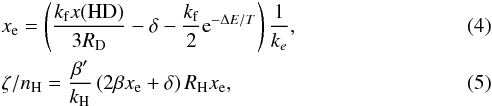
Observations were carried out over 40 h in December, 2011, and March, 2012, with the IRAM 30 m telescope. We used the EMIR bands with the Fast Fourier Transform Spectrometer as a backend in the position-switching mode, using OFF positions about 1000′′ to the east. Amplitude calibration was done typically every 15 min, and pointing and focus were checked every 1 and 3 h, respectively, ensuring ≈2′′ pointing accuracy. All spectra were reduced using the CLASS package of the GILDAS1 software (Pety 2005). Residual bandpass effects were subtracted using low-order (≤3) polynomials. The weather was good and Tsys values were lower than 220 K. The observed molecular transitions used in the present work are listed in Table 1, along with the associated system temperature and sensitivity ranges Tsys and σrms obtained during the successive runs of observations. All spectra are presented on the main-beam temperature scale, 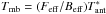 , with Feff and Beff the forward and main-beam efficiencies of the telescope, respectively.
We observed towards 16 positions, of which 10 are located in the northern cloud and 6 in the southern cloud. The coordinates of these positions are listed in Table 2. The two lowest rotational transitions of 13CO and C18O are used to derive the physical conditions in the cloud, while H13CO+(1−0) and DCO+(2−1) are used to derive the cosmic ray ionisation rate.
J2000 coordinates of the 16 observed positions.
4. Results
4.1. Observed spectra
The resulting spectra towards all positions are shown in Fig. 2. The 13CO and C18O spectra show multiple velocity components, most likely associated with several clouds along the line of sight. In some instances, negative features are apparent, which are due to emission from the reference position at different velocities. Isotopologues 13CO and C18O are detected towards 12 of the 16 positions, and the spectra show clearly two main components. The velocity of the dominant component varies between the northern (≲21 km s-1) and southern (≳7 km s-1) cloud, as presented in Sect. 2. At most positions, the rarer C17O isotopologue is also detected, although the hyperfine structure of the (1−0) transition is not always well resolved. The H13CO+(1−0) and DCO+(2−1) emission lines have only one velocity component, at 21 km s-1. The C18O(1−0) and (2−1) lines show a clear distinction between the northern positions, where the line emission is the strongest, and southern positions. The compound H13CO+ is detected towards all northern positions but N8. However, DCO+ is detected only towards three positions, N2, N5, and N6. Southern positions display much weaker emission and SE1 is detected in both H13CO+ and DCO+.
The analysis was essentially driven by the H13CO+ and DCO+ lines which are the main focus of the present work. The velocity of the dominant CO transition always corresponds to the velocity of the H13CO+ line when detected. When more velocity components are detected in CO, we limited the Gaussian fits to the first two dominant components. Upper limits are given at the 1σ level for Tpeak, and for the integrated intensity W by assuming Δv = 3 km s-1. The results from the Gaussian fits are summarised in Table 3 (CO isotopologues) and Table 4 (H13CO+, DCO+).
In the following, we describe the two-step analysis of the measured line intensities. First, the physical conditions are derived according to the 13CO and C18O lines. Second, the HCO+/DCO+ abundance ratio is compared with model predictions computed using the derived physical conditions.
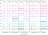 |
Fig. 2 Observations of millimetre emission lines towards all positions. The intensities are in units of main-beam temperature (K). For readibility, a multiplicative factor was applied to the spectra and is given under each transition line label. This factor was decreased for position N2 (protostar) where the signal is very strong. Vertical dashed lines indicate the two extreme velocity components of the complex at 7 and 21 km s-1. |
Results from the Gaussian fits of the emission lines of 13CO and C18O towards the 12 positions where they are detected.
4.2. Determination of physical conditions
The physical conditions prevailing at the various locations were determined based on the 13CO (1−0) and (2−1) lines and the C18O (1−0) and (2−1) lines. To accomplish this, we performed non-local thermal equilibrium (non-LTE) calculations of the rotational level populations under the large velocity gradient (LVG) approximation (Ceccarelli et al. 2003). The H2 density, gas kinetic temperature Tkin, and total column density of each species covered a large parameter space. For each set of input parameters, the expected line intensities and integrated intensities were computed adopting the linewidth Δv derived from the Gaussian fits (Table 3), and taking into account beam dilution effects by varying the size of the emitting regions. A simple χ2 minimization was then used to constrain the physical conditions that best reproduce the observed intensities. The LVG analysis was performed towards positions where all four lines were detected. We considered collisions of 13CO and C18O with both para and ortho H2, assuming an ortho-to-para ratio in Boltzmann equilibrium. Hence, in the temperature range considered here, H2 is mainly in its para configuration. We used the collisional cross sections from Yang et al. (2010).
In this process, the relative abundances of C18O to 13CO need to be known, and we have assumed that the molecular isotopic ratios are equal to the elemental isotopic ratios, namely that ![Mathematical equation: \begin{equation} \frac{[\cdo]}{[\thco]} = \frac{[\cdo]}{[\docseo]} \times \frac{[\docseo]}{[\thco]} \approx \left(\frac{\huo}{\seo}\right) \times \left(\frac{\doc}{\trc}\right)\cdot \end{equation}](/articles/aa/full_html/2014/08/aa24036-14/aa24036-14-eq55.png) (1)It is known that isotopic ratios may vary with the position within the Milky Way, resulting from the gradual depletion of 12C and enrichment of 13C with the cycling of gas through stars (e.g. Wilson & Rood 1994; Frerking et al. 1982). In addition, local variations are also possible, resulting from the competition of chemical fractionation and selective photodissociation (van Dishoeck & Black 1988; Federman et al. 2003). The dependence of the 12C/13C isotopic ratio on galactocentric distance was studied by Milam et al. (2005). Applying their results to W28, which is 4−6 kpc from the Galactic center, one gets 12C /13C = 50 ± 7. In practice, in our non-LTE analysis, we varied the 13C /12C ratio. The best χ2 values were obtained using an isotopic ratio of 50, consistent with the above expectation, which we therefore adopted in what follows. Regarding the 16O /18O isotopic ratio, we adopted the value of 500 representative of the solar neighborhood.
(1)It is known that isotopic ratios may vary with the position within the Milky Way, resulting from the gradual depletion of 12C and enrichment of 13C with the cycling of gas through stars (e.g. Wilson & Rood 1994; Frerking et al. 1982). In addition, local variations are also possible, resulting from the competition of chemical fractionation and selective photodissociation (van Dishoeck & Black 1988; Federman et al. 2003). The dependence of the 12C/13C isotopic ratio on galactocentric distance was studied by Milam et al. (2005). Applying their results to W28, which is 4−6 kpc from the Galactic center, one gets 12C /13C = 50 ± 7. In practice, in our non-LTE analysis, we varied the 13C /12C ratio. The best χ2 values were obtained using an isotopic ratio of 50, consistent with the above expectation, which we therefore adopted in what follows. Regarding the 16O /18O isotopic ratio, we adopted the value of 500 representative of the solar neighborhood.
The results of the LVG analysis are summarised in Table 5. At each position, the size of the emitting regions was found to be larger than the beam size. Position N2, which is considered a protostar in Lefloch et al. (2008), shows a peculiar behaviour with a visual extinction at least 5 times higher than for the other positions. Overall, the density and kinetic temperature we derived are typical of dense molecular clouds with visual extinctions larger than 10 mag. We also note that the H2 densities we derived in the northern cloud are consistent with values published by Lefloch et al. (2008).
4.3. The DCO+/HCO+ abundance ratio
The species DCO+ was detected towards four positions, for which it was possible to derive values of the DCO+/ HCO+ abundance ratio. For all other positions where H13CO+ was detected, upper limits at the 1σ level on the abundance ratio we derived. We determined the column densities of H13CO+ and DCO+ from the same non-LTE LVG calculation, using the collisional cross sections from Flower (1999) and the physical conditions derived from the CO observations (Table 5). We derived the observed DCO+/ HCO+ abundance ratio for each set of physical conditions (nH2,T), assuming 12C /13C = 50 (see Sect. 4.2). The uncertainty in the abundance ratio is dominated by the uncertainties in the physical conditions. Results are listed in Table 5 and will be used in the next section to constrain the CR ionisation rate.
5. Methods to measure the CR ionisation rate ζ
5.1. Analytical method
In their seminal paper, Guélin et al. (1977, hereafter G77) suggested that the abundance ratio of DCO+ to HCO+, which we denote RD = DCO+/ HCO+, can be used to measure the ionisation fraction in molecular clouds, xe = n(e−) /nH. Subsequently, Caselli et al. (1998, hereafter C98) proposed using the RH = HCO+/ CO abundance ratio in combination with RD to derive both xe and ζ in dark clouds. The basic idea is that DCO+ and HCO+ are chemically linked, and depend on a reduced number of chemical reactions where the CR ionisation rate plays a crucial role, through the ionisation of H2 into H (Herbst & Klemperer 1973), leading to the formation of the pivotal H
 ion. The fast ion-neutral reaction of H with HD produces the deuterated ion H2D+ which then initiates the formation of several deuterated species, including DCO+. In a similar fashion, HCO+ is formed by the reaction of H with CO. This forms the basis of the method of C98 which uses CO, DCO+, and HCO+ to derive xe and ζ. The full set of reactions used in the C98 analysis is given in Table A.1 with updated reaction rates.
The steady-state abundance ratios RH = HCO+/ CO and RD = DCO+/ HCO+ can be analytically derived from this network, provided that HCO+ and DCO+ are predominantly formed and destroyed by reactions 1−4 and 7−9, respectively. One then finds that ![Mathematical equation: \begin{equation} \label{eq:RH} R_{\rm H} = \frac{[\hcop]}{[\co]} = \frac{k_{\rm H}}{\beta'} \frac{x(\htrp)}{\xe} \approx \frac{k_{\rm H}}{(2 \beta \xe + \delta) \beta'}\frac{\zeta/n_\h}{\xe} , \end{equation}](/articles/aa/full_html/2014/08/aa24036-14/aa24036-14-eq69.png) (2)and
(2)and ![Mathematical equation: \begin{equation} \label{eq:RD2} \rd = \frac{[\dcop]}{[\hcop]} \approx \frac{1}{3}\frac{x(\hhdp)}{x(\htrp)} \approx \frac{1}{3} \frac{k_{\rm f} x(\hd)}{k_{\rm e} \xe+\delta+k_{\rm f}^{-1}/2}, \end{equation}](/articles/aa/full_html/2014/08/aa24036-14/aa24036-14-eq70.png) (3)where n(X) is the number density of species X and x(X) = n(X) /nH its fractional abundance. In the following, we will assume that the gas is fully molecular such that nH = 2n(H2). The coefficients β, β′, and k are the reaction rates listed in Table A.1. Finally,
(3)where n(X) is the number density of species X and x(X) = n(X) /nH its fractional abundance. In the following, we will assume that the gas is fully molecular such that nH = 2n(H2). The coefficients β, β′, and k are the reaction rates listed in Table A.1. Finally,  is the total destruction rate of or H2D+ by neutrals. Provided that RH, RD, nH, and the kinetic temperature are known, xe and ζ can then be derived as
 where ΔE = 220 K, such that at sufficiently low temperatures the last term in brackets in Eq. (4) becomes negligible. Equation (4) demonstrates that xe only depends on the abundance ratio RD and the gas kinetic temperature, as originally proposed by G77.
Results from the Gaussian fits of the emission lines of H13CO+ and DCO+ towards the nine positions where H13CO+ is detected.
Figure 3 shows xe as a function of RD, as predicted from Eq. (4), assuming a kinetic temperature of 20 K (blue dashed line). We note two regimes in the dependence of xe on RD. For low RD values (≲10-2), xe is proportional to 1 /RD with a factor that depends on the chemical reaction rates and the HD abundance. For higher RD values, xe drops sharply. In this regime, xe varies by more than two orders of magnitude when RD is changed by only a factor of two. The slope becomes steeper with increasing temperature, due to the predominance of the reverse reaction of the formation of H2D+ (Table A.1). This indicates that accurate values of xe in dark clouds through this method require extremely accurate values of RD. It also suggests that in regions with higher ionisation, where xe is proportional to 1 /RD, DCO+ will be difficult to detect.
Physical conditions and cosmic ray ionisation rates.
5.2. Numerical models
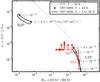 |
Fig. 3 xe = n(e−) /nH as a function of RD. Values from the analytical method (G77) in Sect. 5.1 are given at T = 20 K (dashed line). Results from our calculation (see Sect. 5.2) for temperatures between 7 K and 20 K are contained within the solid lines. ζ values are given for nH = 104 cm-3, although the model only depends on the ζ/nH ratio (see text). RD values or upper limits as derived from observations are indicated by the red symbols; see Sect. 6.1. |
To assess the validity of the analytical approach of G77 and C98, we have solved the OSU 20092 chemical network for the abundances of DCO+, HCO+, and e−, using the astrochem3 code. The time evolution of the gas-phase abundances was followed until a steady state was reached, after typically 10 Myr. The underlying hypothesis is that the cloud was already molecular when it was irradiated by the CRs emitted at the SN explosion. The chemical changes caused by the sudden CR irradiation are dominated by ion-neutral reactions, whose timescale is only ~102 yr, much shorter than the W28 SNR age (~104 yr; see Introduction). Details of the models are given in Appendix A. In one calculation, the gas is shielded by 20 mag of visual extinction, such that UV photons can safely be ignored.
As anticipated from Eq. (2), we found that the abundances mostly depend on the ζ/nH ratio, rather than on ζ and nH separately. This behaviour is similar to photon-dominated regions in which a good parameter is the ratio of the UV radiation field to the total density. For each temperature from 7 K to 20 K, a series of calculations with ζ/nH increasing from 10-22 cm3 s-1 to 10-18 cm3 s-1 were performed, and the steady-state values of xe and RD were recorded.
In these calculations, we assumed a standard CO abundance of ~7.3 × 10⁻⁵ in the cloud. Indeed, since the density of the studied clouds is relatively low (Table 5), we do not expect CO depletion to play an important role here. However, in general, one has to take into account this uncertainty. In addition, our calculations do not consider separately the H2 ortho-to-para ratio, which is known to affect the DCO+/HCO+ abundance ratio when it is larger than about 0.1 (e.g. Pagani et al. 2011). Our choice here is based on the published observations that indicate that the H2 ortho-to-para ratio is smaller than about 0.01 in molecular clouds (e.g Troscompt et al. 2009; Dislaire et al. 2012).
5.3. A new view of the DCO+/HCO+ method
The results of the numerical models are shown in Fig. 3. As expected, the ionisation fraction xe increases with ζ/nH, with RD decreasing in the process. There is good overall agreement between the analytical and numerical predictions for RD ≳ 2 × 10⁻². In this high-RD regime, the small differences between analytical and numerical values are due to the abundances of HD and CO not being constant as originally assumed by G77 and C98. Instead, as ζ/nH and xe increase, atomic deuterium becomes more abundant. Similarly, the CO abundance decreases because of the dissociating action of CRs. When RD decreases and reaches ≈2 × 10⁻², the abundances predicted by the numerical model change dramatically to a regime characterised by large values of xe and low values of RD. This jump corresponds to the well-known transition from the so-called low ionisation phase (LIP) to the high ionisation phase (HIP) (Pineau des Forêts et al. 1992; Le Bourlot et al. 1993), and is due to the sensitivity of interstellar chemical networks to ionisation. The LIP is associated with RD larger than 10-2, whilst the HIP is characterised by RD ≲ 10-4. In our calculations, the LIP-HIP transition occurs at ζ/nH ~ 3 × 10-19 cm3 s-1, and we note that this value depends only slightly on the temperature, although it is known to depend on other parameters such as the gas-phase abundance of metals (Wakelam et al. 2006a). A detailed analysis of the LIP-HIP transition is, however, not the aim of this study. Here, it is rather the existence of this instability which is of interest since it produces a sharp difference between the analytical and the numerical predictions from the ionisation point of view. Application to a practical case shows that what changes is not the jump itself but (slightly) the ζ at which it occurs (see e.g. Ceccarelli et al. 2011). In the former, the variations of xe and RD are continuous and, as already mentioned, predict xe ~ 1 /RD in the low-RD regime. This scaling is, however, not observed in the numerical models, and is replaced by a discontinuous variation of both xe and RD. The present calculations show that the LIP is characterised by RD = 10-2− 10-1, xe ≲ 5 × 10⁻⁷, and the HIP is characterised by RD ≈ few 10-5 and xe ≈ few 10-5.
As shown in Fig. 4, the low values of RD in the HIP are due to a very low abundance of DCO+, whilst the abundance of HCO+ decreases by a smaller amount. This has important consequences when using the DCO+/HCO+ method to derive the ionisation fraction and CR ionisation rate. First, it must be recognised that this method may provide a value of xe only for LIP-dominated gas conditions. In other words, where DCO+ is detected, the line of sight is dominated by low-xe gas. For lines of sight dominated by HIP gas, the abundance of DCO+ is expected to be well below detectable thresholds, such that only upper limits on RD can be derived. Yet, an upper limit on RD still provides essential information, since it is associated with a lower limit on xe, which in turn corresponds to a lower limit of ζ/nH. On the contrary, for LIP-dominated lines of sight, the value of xe and ζ/nH may be derived directly from RD, although xe is extremely sensitive to uncertainties on RD in this regime.
6. The CR ionisation rate in W28
6.1. Constant density and temperature cloud analysis
A new view of the DCO+/HCO+ method thus emerges, which stresses its strengths and limitations. The method allows the determination of the ionisation fraction xe and the ζ/nH ratio for gas in the LIP, and provides lower limits of xe and ζ/nH for gas in the HIP. In the following, we apply this method to the sample of observed points, using the constraints on the gas temperature and density, and the RD value in each point (Table 5). We emphasise that the model calculations summarised in Fig. 3 assumed constant density and gas temperature. In the next section, we will discuss how the DCO+/HCO+ method can be used to constrain xe and ζ/nH, taking into account the thermal structure of the cloud.
Of the 16 lines of sight initially observed in CO, 12 were also detected in H13CO+, of which 4 led to RD determinations and 5 to upper limits (Table 5). The four points with measured RD are N5, N6, SE1, and N2. In the following analysis, we exclude N2 as it coincides with a protostar, which means that a more accurate analysis taking into account the structure of the protostar and the inner ionisation is necessary. The values obtained towards N5, N6, and SE1 are shown in Fig. 3.
The SE1 point lies on the LIP branch, enabling a determination of the ionisation fraction xe = (0.15−4) × 10-7 and of the CR ionisation rate ζ = (0.2−20) × 10-17 s-1. On the contrary, the values of RD towards N5 and N6 lie in the gap between the LIP and HIP branches, even when considering a kinetic temperature as high as 20 K, a temperature which is larger than the values derived for these positions. In these cases, adopting nH = 2n(H2) ≳ 4 × 103 cm-3 (Table 5), Fig. 3 provides the following lower limits: xe ≳ 4 × 10⁻⁷ and ζ ≳ 1.3 × 10⁻¹⁵ s-1 for both points. We note that the detection of DCO+ indicates that the line of sight includes a non-negligible amount of LIP, which can serve to further constrain the value of ζ/nH. This can be seen in Fig. 4, which shows RD and DCO+ as a function of ζ, for a density and temperature appropriate to position N5 (Table 5). The measured RD intersects the model predictions at the edge of the LIP/HIP jump, at ζ ≈ 2.5 × 10⁻¹⁵ s-1. More importantly, the figure shows that the gas is neither entirely in the LIP nor HIP state as expected from the detection of DCO+. A similar plot has also been obtained for N6, leading to the same conclusion.
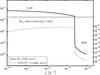 |
Fig. 4 RD = DCO+/ HCO+ (thick line, left axis) and x(DCO+) = n(DCO+) /nH (dashed line, right axis) as a function of ζ, for T = 10 K and nH = 8 103 cm-3, i.e. the physical conditions characterising position N5. The HIP and LIP are marked. The hatched area shows the range of observed RD at that position. |
Finally, the non-detection of DCO+ in the other lines of sight leads to upper limits on RD that are well outside the LIP branch. At these positions, the gas is very likely to be almost entirely in the HIP state, which means that ζ/nH ≳ 3 × 10-19 cm3 s-1. An exception is the point SW4, where an extremely energetic outflow has been detected (Harvey & Forveille 1988), and where the HCO+ is therefore likely contaminated by the outflowing material.
6.2. Constant density cloud analysis
As discussed in the previous section, the points N5 and N6 are likely composed of a mixture of gas in the LIP and HIP state. This is similar to the situation observed in W51C-E (CC2011). In that case, ζ was estimated with a model that takes into account the thermal and chemical structure of a constant density cloud, where a fraction (the deepest) is in the LIP and the rest in the HIP (Fig. 2 in CC2011). Here, we do a similar analysis, using basic arguments instead of a sophisticated model, and we show that it leads to similar results, namely the determination of ζ to within a factor of 2. The advantage of this analysis is that it shows in a straightforward way the uncertainty due to the model parameters.
The crucial point is understanding what causes the gas to flip from the HIP to the LIP state going deeper into the cloud. Since the column density is too low to appreciably reduce ζ across the cloud, the only macroscopic quantity that changes is the gas temperature. Specifically, the temperature increases by a few K (in the UV-shielded region) going deeper into the cloud because the CO line opacity increases and, consequently, the line cooling becomes less efficient. The effect is larger for larger ζ as the heating, dominated by the CR ionisation, is less compensated by the line cooling.
It is instructive to see how the RD ratio changes as a function of the gas temperature for different ζ. This is shown in Fig. 5, for a range of temperatures (5−80 K) and ζ/nH (2–5 × 10-19 cm3 s-1, appropriate to the N5 and N6 points). In these calculations, we consider a cell of gas of constant density, shielded by 20 mag of visual extinctions as before, such that the ionisation is driven by the CRs. The figure shows important features:
-
i)
for ζ/nH ≲ 2 × 10-19 cm3 s-1, the cloud is always in the LIP, regardless of the temperature;
-
ii)
for ζ/nH ≳ 5 × 10-19 cm3 s-1, the cloud is always in the HIP for temperatures lower than 50 K;
-
iii)
for intermediate values of ζ/nH, the gas flips from HIP to LIP with increasing temperature, and the larger ζ is, the larger the temperature where the flip occurs.
These calculations show that there is a range of ionisation rates in which the gas is extremely sensitive to temperature variations. A tiny increase in temperature is sufficient to make the gas flip from the HIP to the LIP. In particular, for position N5, there is such a combination of values of RD, Tkin, and ζ/nH (see Fig. 5) that places it precisely in a region where the transition from HIP to LIP can be triggered by an increase in Tkin as small as a few K. A similar argument applies to N6. In addition, in regions exposed to an enhanced CR ionisation rate, the outer part characterised by large ionisation fractions will be extended farther into the cloud, thus decreasing the relative amount of LIP with respect to the HIP.
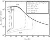 |
Fig. 5 RD as a function of the gas temperature Tkin for different values of ζ/nH: from 2 to 5 × 10-19 s-1, as marked. Note that for ζ/nH ≤ 2 × 10-19 cm3 s-1 (thick solid line), the cloud is always in the LIP, regardless of the temperature. For ζ/nH> 5 × 10-19 cm3 s-1 (thin dashed curve), the cloud is always in the HIP for temperatures ≤50 K. Hatched areas show observations of N5 and N6. We assume AV = 20 mag. |
Based on the derived kinetic temperatures and values of RD (Table 5) and using Fig. 5, we can further constrain the value of ζ/nH. Towards N5, the temperature was found to be 10 ± 2 K, while RD = 0.014−0.020. When inserted into Fig. 5, these delineate a region that is compatible with a narrow range of ζ/nH = (2.8−3.0) × 10-19 cm3 s-1. For the N6 line of sight, we find similar values, (2.9−3.2) × 10-19 cm3 s-1. The densities derived from the analysis and their uncertainties then lead to cosmic ray ionisation rates of (1.3−3.3) × 10-15 s-1 and (1.3−4.0) × 10-15 s-1 for N5 and N6 respectively. Results are summarised in Table 5 and are included in Figs. 6 and 7.
7. Discussion
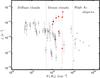 |
Fig. 6 Compilation of measured ζ in different objects (open squares), as reported by Padovani & Galli (2013). The black filled square denotes W51 (Ceccarelli et al. 2011). Red points and lower limits report the values derived in this work. The dashed lines show the range of column densities (0.5−10) × 1022 cm-2, typical of dense molecular clouds, corresponding to visual extinctions of 5 and 100 mag, respectively. On the left lie the diffuse clouds and on the right highly obscured environments such as infrared dark clouds or protoplanetary discs. |
Table 5 lists the observed positions and the corresponding CR ionisation rates derived using the method described in the previous section. With the exception of the SE1 point, in all other points ζ is at least 10 to 260 times larger than the standard value (1 × 10-17 s-1) in Galactic clouds. This is shown in Fig. 6, where we present a compilation of the ζ measured in various objects (from Padovani & Galli 2013), plus our measurements. In the range of column densities (0.5−10) × 1022 cm-2, typical of dense molecular clouds, the points in which we derived ζ are those with the highest values, together with the CC2011 point (filled square). The first conclusion of this work is, therefore, that clouds next to SNR are indeed irradiated by an enhanced flux of CRs of relatively low energy (see below for a more quantitative statement on the CR particle energies).
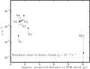 |
Fig. 7 CR ionisation rate ζ as a function of the approximate projected distance from the SNR radio boundary (blue circle in Fig. 1), assuming a W28 distance of 2 pkc. We note that the ζ error bars are dominated by the uncertainties on the H2 densities (see text). |
The dependence of ζ on the projected distance from the SNR radio boundary (assuming a W28 distance of 2 kpc) is shown in Fig. 7. Remarkably, the point farthest (~10 pc) from the SNR edge is the one with the lowest ζ. Actually, it is the only point where the gas is predominantly in the LIP state. All other points, at distances ≲3 pc, have at least a fraction of the gas in the HIP, namely they have a larger xe and ζ. Of course, this analysis does not take into account the 3D structure of the SNR complex. Yet, this can still provide us with constraints on the propagation properties of CRs, as will be discussed in the following.
Valuable additional information is provided by observations in the γ-ray domain. Both the northern and southern clouds coincide with sources of TeV emission, as seen by HESS. This means that the clouds are illuminated by very high energy (≳10 TeV) CRs, which already escaped the SNR expanding shell and travelled the ≳10 pc (or more, if projection effects play a role) to the southern cloud. Conversely, the low CR ionisation rate measured in SE1 tells us that the ionising lower energy CRs remain confined closer to the SNR. In the same vein, GeV emission has been detected towards the northern region but only towards a part of the southern one. This difference between the GeV and TeV γ-ray morphology has been interpreted as a projection effect: the portion of the southern region that exhibits a lack of GeV emission is probably located at a distance from the shock significantly larger than the projected one, >10 pc, and thus can be reached by ≳TeV CRs but not by ≳GeV ones (Gabici et al. 2010; Li & Chen 2010; Nava & Gabici 2013). Remarkably, the SE1 point is located in the region where the lack of GeV emission is observed.
The picture that emerges is that of a stratified structure with CRs of larger and larger energies occupying larger and larger volumes ahead of the shock. Within this framework, it is possible to estimate the CR diffusion coefficient in the region. This can be done by recalling that in a given time t, CRs diffuse over a distance  , where D is the energy dependent diffusion coefficient. For the situation under examination, one gets
 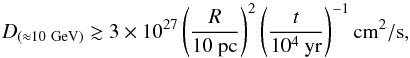 (6)where D(≈ 10 GeV) is the diffusion coefficient of ≈10 GeV CRs, which are those responsible for the ≈GeV γ-ray emission, and t is the time elapsed since the escape of CRs from the SNR. The value obtained in Eq. (6) is in substantial agreement with more accurate studies (see e.g. Nava & Gabici 2013).
The diffusion coefficient obtained in Eq. (6) can then be rescaled to lower energies, according to D ∝ psβ, where p is the particle momentum, β = v/c its velocity in units of the speed of light, and s depends on the spectrum of the ambient magnetic turbulence. The typical value of s in the interstellar medium is poorly constrained to be in the range 0.3 to 0.7 (Castellina & Donato 2011). In the following, we adopt s = 0.5. To estimate the diffusion length of low energy CRs, one has to keep in mind that, while CRs with energies above ≈GeV are virtually free from energy losses (the energy loss time for proton–proton interactions in a density nH ≈ 103 cm-3 is comparable to the age of the SNR), lower energy CRs suffer severe ionisation losses over a short timescale (Berezinskii et al. 1990): 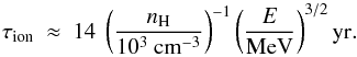 (7)This approximate expression is sufficiently accurate in the range of energies spanning 1−100 MeV. The diffusion length of low energy CRs can then be estimated by equating the diffusion time
  to the energy loss time τion, which gives Rd ≈ 0.02, 0.3, and 3 pc for CRs of energy 1, 10, and 100 MeV, respectively. This implies that only CRs with energies ≳100 MeV can escape the shock and spread over a distance of 3 pc or more, and thus these are the CRs that play a major role in ionising the gas. Whether the ionisation of the gas is due directly to these CRs or to the products of their interaction with the gas (namely slowed down lower energy CRs) remains an open question. It is remarkable that the particle energies of ionising CRs (≈0.1−1 GeV) also make them capable of producing sub–GeV γ rays, given that the kinetic energy threshold for π0 production is ≈280 MeV.
Of course, the order of magnitude estimates discussed in this section cannot substitute in any way more sophisticated calculations, yet they clearly indicate an intriguing possible link between low and high energy observations of SNR environments. In fact, in the scenario described above, the very same CRs are responsible for both ionisation of the gas and production of low energy γ rays. If confirmed, such a link would constitute robust evidence for the presence of accelerated protons in the environment of the SNR W28, a thing that would bring further support to the idea that SNR are the sources of Galactic CRs. Additional theoretical investigations are needed in order to examine and possibly rule out alternative scenarios which may include other contributions to the ionisation rate (e.g. CR electrons, X-ray photons) or different means of propagation (e.g. straight-line or advective propagation of low energy CRs).
8. Conclusion
In this work, we presented new observations to measure the CR ionisation rate in molecular clouds close to supernova remnants (SNR). In doing so, the DCO+/HCO+ method was also revisited. The major results may be summarised as follows.
-
1)
We observed the two lowest rotational transitions of13CO and C18O towards 16 positions in the northern and southern clouds close to theSNR W28. The four lines were detected in emission towards 12 of these positions, where we could, therefore, derive the physical conditions using a non-LTE LVG analysis. With the exception of one position (N2) coinciding with a proto-star in the region, we derived H2 densities and temperatures typical of molecular clouds, namely nH2 = (0.2−10) × 103 cm-3 and T = 6−24 K. We searched for H13CO+ and DCO+ line emission in the above 12 positions, and detected it in 9 and 4, respectively. From these data, we could derive the RD = DCO+/ HCO+ in 4 positions, one of which coincides with the protostar, and give upper limits for the remaining 5 positions.
-
2)
We reinvestigated the DCO+/HCO+ method used to derive the ionisation fraction xe = n(e−) /nH and the relevant CR ionisation rate ζ causing it. To this aim, we compared the steady-state abundances of HCO+, DCO+, and e− as predicted by the analytical model of G77, to numerical calculations, assuming constant density and gas temperature. The numerical model leads to two well separated regimes of ionisation, also known as the low- and high-ionisation phases (LIP and HIP; Pineau des Forêts et al. 1992). In the context of this work, these two phases lead to two separated regimes in terms of ζ and RD values:
-
i)
for ζ/nH ≲ 3 × 10-19 cm3 s-1, the gas is in the LIP, where RD ≳ 2 × 10⁻² and xe ≲ 6 × 10⁻⁷. In this regime, the dependence of xe on RD is very steep leading to large uncertainties on xe;
-
ii)
for ζ/nH ≳ 3 × 10-19 cm3 s-1, the gas is in the HIP, where RD ≲ 10-4 and xe ≳ 2 × 10⁻⁵. In this regime, DCO+ is not detectable and the numerical prediction for xe differs significantly from the analytical one.
Therefore, the DCO+/HCO+ abundance ratiocan provide a measure of xe and ζ in the LIP, and only lower limits if the gas is in the HIP.
-
i)
-
3)
We found only one position, SE1, in the LIP, where RD = 0.032−0.05, xe = (0.3−4) × 10-7 and ζ = (0.2−20) × 10-17 s-1. Two positions, N5 and N6, lie in the gap between the LIP and HIP, namely the gas is neither entirely in the LIP nor in the HIP, although it certainly contains a fraction of gas in the LIP, where DCO+ is detectable (and detected). The jump from the HIP to the LIP when penetrating farther into the cloud is associated with an increase in the temperature, and we showed that model calculations at several temperatures further constrain the value of ζ. The uncertainty in ζ towards these positions is dominated by the uncertainty in the H2 density and the derived values are ζ = (1.3−3.3) and (1.3−4.0)× 10-15 s-1 for N5 and N6, respectively. Towards the remaining 5 positions with upper limits on RD, the derived ζ values are at least 10 to 260 times higher than the standard value of 1 × 10-17 s-1.
-
4)
The points of the northern cloud have the largest CR ionisation rates measured so far in the Galaxy. The point towards the southern cloud is, on the contrary, consistent with the average galactic CR ionisation rate of molecular clouds not interacting with a SNR. Since the northern and southern clouds have projected distances from the SNR shock of ≤3 and ~10 pc, respectively, this can be explained by the fact that the low energy ionising CRs have not reached the southern cloud yet. On the other hand, the observations show that both the northern and southern clouds coincide with TeV emission sources, suggesting that high ≳10 TeV CRs have reached both. This is also consistent with γ-ray emission sources inciding with the northern cloud but only partially with the southern cloud, indicating that the former is irradiated by ≈0.1−1 GeV CRs, while only the nearest portion of the southern cloud is so affected.
-
5)
The emerging picture is that of energy-dependent diffusion properties of hadronic CRs. The high-energy CRs responsible for TeV γ-ray emission through π0-decay can diffuse far ahead of the SNR shock, while the low-energy CRs (0.1−1 GeV), responsible for both the low γ-ray emission and the ionisation of the gas, remain closer to the SNR shock. The present work thus gives first observational evidence to the theoretical predictions that hadrons of energy 0.1−1 GeV contribute most to the ionisation in dense gas (Padovani et al. 2009).
Acknowledgments
We warmly thank Marco Padovani for providing us with his compilation and for useful discussions. This work has been financially supported by the Programme National Hautes Énergies (PNHE). Based on observations carried out with the IRAM 30 m telescope. IRAM is supported by INSU/CNRS (France), MPG (Germany) and IGN (Spain). S. Gabici acknowledges the financial support of the UnivEarthS Labex Program at Sorbonne Paris Cité (ANR-10-LABX-0023 and ANR-11-IDEX-0005-02).
References
- Abdo, A. A., Ackermann, M., Ajello, M., et al. 2010, ApJ, 718, 348 [Google Scholar]
- Abdo, A. A., Ackermann, M., Ajello, M., et al. 2011, ApJ, 734, 28 [NASA ADS] [CrossRef] [Google Scholar]
- Ackermann, M., Ajello, M., Allafort, A., et al. 2013, Science, 339, 807 [NASA ADS] [CrossRef] [PubMed] [Google Scholar]
- Aharonian, F. A. 2013, Astropart. Phys., 43, 71 [NASA ADS] [CrossRef] [Google Scholar]
- Aharonian, F., Akhperjanian, A. G., Bazer-Bachi, A. R., et al. 2008, A&A, 481, 401 [NASA ADS] [CrossRef] [EDP Sciences] [MathSciNet] [PubMed] [Google Scholar]
- Arikawa, Y., Tatematsu, K., Sekimoto, Y., & Takahashi, T. 1999, PASJ, 51, L7 [Google Scholar]
- Asplund, M., Grevesse, N., Sauval, A. J., & Scott, P. 2009, ARA&A, 47, 481 [NASA ADS] [CrossRef] [Google Scholar]
- Balbus, S. A., & Hawley, J. F. 1998, Rev. Mod. Phys., 70, 1 [Google Scholar]
- Bell, A. R. 1978, MNRAS, 182, 147 [NASA ADS] [CrossRef] [Google Scholar]
- Berezinskii, V. S., Bulanov, S. V., Dogiel, V. A., & Ptuskin, V. S. 1990, Cosmic ray astrophysics (Amsterdam: North Holland) [Google Scholar]
- Boger, G. I., & Sternberg, A. 2006, ApJ, 645, 314 [NASA ADS] [CrossRef] [Google Scholar]
- Bolatto, A. D., Wolfire, M., & Leroy, A. K. 2013, ARA&A, 51, 207 [Google Scholar]
- Brogan, C. L., Gelfand, J. D., Gaensler, B. M., Kassim, N. E., & Lazio, T. J. W. 2006, ApJ, 639, L25 [NASA ADS] [CrossRef] [Google Scholar]
- Caselli, P., Walmsley, C. M., Terzieva, R., & Herbst, E. 1998, ApJ, 499, 234 [Google Scholar]
- Castellina, A., & Donato, F. 2011, Planets, Stars and Stella Systems (Springer-Verlag) [arXiv:1110.2981] [Google Scholar]
- Ceccarelli, C., Maret, S., Tielens, A. G. G. M., Castets, A., & Caux, E. 2003, A&A, 410, 587 [NASA ADS] [CrossRef] [EDP Sciences] [Google Scholar]
- Ceccarelli, C., Hily-Blant, P., Montmerle, T., et al. 2011, ApJ, 740, L4 [Google Scholar]
- Claussen, M. J., Frail, D. A., Goss, W. M., & Gaume, R. A. 1997, ApJ, 489, 143 [NASA ADS] [CrossRef] [Google Scholar]
- Dame, T. M., Hartmann, D., & Thaddeus, P. 2001, ApJ, 547, 792 [NASA ADS] [CrossRef] [Google Scholar]
- Dislaire, V., Hily-Blant, P., Faure, A., et al. 2012, A&A, 537, A20 [NASA ADS] [CrossRef] [EDP Sciences] [Google Scholar]
- Elmegreen, B. G. 1998, ASP Conf. Ser., 148, 150 [NASA ADS] [Google Scholar]
- Federman, S. R., Lambert, D. L., Sheffer, Y., et al. 2003, ApJ, 591, 986 [NASA ADS] [CrossRef] [Google Scholar]
- Ferrière, K. M. 2001, Rev. Mod. Phys., 73, 1031 [NASA ADS] [CrossRef] [Google Scholar]
- Flower, D. R. 1999, MNRAS, 305, 651 [NASA ADS] [CrossRef] [Google Scholar]
- Frail, D. A., Goss, W. M., & Slysh, V. I. 1994, ApJ, 424, L111 [NASA ADS] [CrossRef] [Google Scholar]
- Frerking, M. A., Langer, W. D., & Wilson, R. W. 1982, ApJ, 262, 590 [NASA ADS] [CrossRef] [Google Scholar]
- Fukui, Y., Sano, H., Sato, J., et al. 2012a, ARA&A, 746, 82 [Google Scholar]
- Fukui, Y., Sano, H., Sato, J., et al. 2012b, ApJ, 746, 82 [NASA ADS] [CrossRef] [Google Scholar]
- Gabici, S., Casanova, S., Aharonian, F. A., & Rowell, G. 2010, in SF2A-2010: Proc. of the Annual meeting of the French Society of Astronomy and Astrophysics, eds. S. Boissier, M. Heydari-Malayeri, R. Samadi, & D. Valls-Gabaud, 313 [Google Scholar]
- Giuliani, A., Tavani, M., Bulgarelli, A., et al. 2010, A&A, 516, L11 [Google Scholar]
- Goudis, C. 1976, Ap&SS, 45, 133 [NASA ADS] [CrossRef] [Google Scholar]
- Graedel, T. E., Langer, W. D., & Frerking, M. A. 1982, ApJS, 48, 321 [NASA ADS] [CrossRef] [Google Scholar]
- Guélin, M., Langer, W. D., Snell, R. L., & Wootten, H. A. 1977, ApJ, 217, L165 [NASA ADS] [CrossRef] [Google Scholar]
- Harvey, P. M., & Forveille, T. 1988, A&A, 197, L19 [NASA ADS] [Google Scholar]
- Herbst, E., & Klemperer, W. 1973, ApJ, 185, 505 [NASA ADS] [CrossRef] [Google Scholar]
- Hewitt, J. W., Yusef-Zadeh, F., & Wardle, M. 2008, ARA&A, 683, 189 [Google Scholar]
- Hillas, A. M. 2005, J. Phys. G Nucl. Phys., 31, 95 [Google Scholar]
- Ilovaisky, S. A., & Lequeux, J. 1972, A&A, 18, 169 [NASA ADS] [Google Scholar]
- Indriolo, N., & McCall, B. J. 2012, ApJ, 745, 91 [NASA ADS] [CrossRef] [Google Scholar]
- Indriolo, N., Blake, G. A., Goto, M., et al. 2010, ApJ, 724, 1357 [NASA ADS] [CrossRef] [Google Scholar]
- Kaspi, V. M., Lyne, A. G., Manchester, R. N., et al. 1993, ApJ, 409, L57 [NASA ADS] [CrossRef] [Google Scholar]
- Le Bourlot, J., Pineau des Forêts, G., Roueff, E., & Schilke, P. 1993, ApJ, 416, L87 [NASA ADS] [CrossRef] [Google Scholar]
- Le Bourlot, J., Pineau des Forêts, G., & Roueff, E. 1995a, A&A, 297, 251 [NASA ADS] [Google Scholar]
- Le Bourlot, J., Pineau des Forêts, G., Roueff, E., & Flower, D. R. 1995b, A&A, 302, 870 [NASA ADS] [Google Scholar]
- Lee, H. H., Roueff, E., Pineau des Forêts, G., et al. 1998, A&A, 334, 1047 [NASA ADS] [Google Scholar]
- Lefloch, B., Cernicharo, J., & Pardo, J. R. 2008, A&A, 489, 157 [NASA ADS] [CrossRef] [EDP Sciences] [Google Scholar]
- Lesur, G., Kunz, M. W., & Fromang, S. 2014, A&A, 566, A56 [NASA ADS] [CrossRef] [EDP Sciences] [Google Scholar]
- Li, H., & Chen, Y. 2010, MNRAS, 409, L35 [NASA ADS] [CrossRef] [Google Scholar]
- Linsky, J. L., & Wood, B. 1995, in Am. Astron. Soc. Meet. Abstr., 27, 1347 [Google Scholar]
- Lozinskaya, T. A. 1974, Sov. Astron., 17, 603 [NASA ADS] [Google Scholar]
- Lozinskaya, T. A. 1981, Sov. Astron. Lett., 7, 17 [NASA ADS] [Google Scholar]
- McCall, B. J., Huneycutt, A. J., Saykally, R. J., et al. 2003, Nature, 422, 500 [NASA ADS] [CrossRef] [PubMed] [Google Scholar]
- Milam, S. N., Savage, C., Brewster, M. A., Ziurys, L. M., & Wyckoff, S. 2005, ApJ, 634, 1126 [NASA ADS] [CrossRef] [Google Scholar]
- Milne, D. K., & Wilson, T. L. 1971, A&A, 10, 220 [NASA ADS] [Google Scholar]
- Morlino, G., Amato, E., & Blasi, P. 2009, MNRAS, 392, 240 [NASA ADS] [CrossRef] [Google Scholar]
- Nava, L., & Gabici, S. 2013, MNRAS, 429, 1643 [NASA ADS] [CrossRef] [Google Scholar]
- Nicholas, B. P., Rowell, G., Burton, M. G., et al. 2012, ARA&A, 419, 251 [Google Scholar]
- Padovani, M., & Galli, D. 2013, Astrophys. Space Sci. Proc., 34, 61 [Google Scholar]
- Padovani, M., Galli, D., & Glassgold, A. E. 2009, A&A, 501, 619 [NASA ADS] [CrossRef] [EDP Sciences] [Google Scholar]
- Padovani, M., Hennebelle, P., & Galli, D. 2013, in SF2A-2013: Proc. of the Annual meeting of the French Society of Astronomy and Astrophysics. eds. L. Cambresy, F. Martins, E. Nuss, & A. Palacios, 409 [Google Scholar]
- Pagani, L., Roueff, E., & Lesaffre, P. 2011, ApJ, L35 [Google Scholar]
- Pety, J. 2005, SF2A-2005: Semaine de l’Astrophysique Francaise (EDP Sciences), Conf. Ser., 721 [Google Scholar]
- Pineau des Forêts, G., Roueff, E., & Flower, D. R. 1992, MNRAS, 258, 45 [NASA ADS] [CrossRef] [Google Scholar]
- Reynolds, S. P. 2008, ARA&A, 46, 89 [Google Scholar]
- Rho, J., & Borkowski, K. J. 2002, ApJ, 575, 201 [Google Scholar]
- Roberts, H., & Millar, T. J. 2000, A&A, 361, 388 [NASA ADS] [Google Scholar]
- Taquet, V., Ceccarelli, C., & Kahane, C. 2012, ApJ, 748, L3 [NASA ADS] [CrossRef] [Google Scholar]
- Troscompt, N., Faure, A., Maret, S., et al. 2009, A&A, 506, 1243 [NASA ADS] [CrossRef] [EDP Sciences] [Google Scholar]
- van Dishoeck, E. F., & Black, J. H. 1988, ApJ, 334, 771 [NASA ADS] [CrossRef] [Google Scholar]
- Velázquez, P. F., Dubner, G. M., Goss, W. M., & Green, A. J. 2002, AJ, 124, 2145 [NASA ADS] [CrossRef] [Google Scholar]
- Wakelam, V., Herbst, E., & Selsis, F. 2006a, A&A, 451, 551 [NASA ADS] [CrossRef] [EDP Sciences] [Google Scholar]
- Wakelam, V., Herbst, E., Selsis, F., & Massacrier, G. 2006b, A&A, 459, 813 [NASA ADS] [CrossRef] [EDP Sciences] [Google Scholar]
- Westerhout, G. 1958, Bull. Astron. Inst., 14, 215 [Google Scholar]
- Wilson, T. L., & Rood, R. 1994, ARA&A, 32, 191 [NASA ADS] [CrossRef] [Google Scholar]
- Wootten, A. 1981, ApJ, 245, 105 [NASA ADS] [CrossRef] [Google Scholar]
- Yang, B., Stancil, P. C., Balakrishnan, N., & Forrey, R. C. 2010, ApJ, 718, 1062 [NASA ADS] [CrossRef] [Google Scholar]
- Yusef-Zadeh, F., Shure, M., Wardle, M., & Kassim, N. 2000, ApJ, 540, 842 [NASA ADS] [CrossRef] [Google Scholar]
Appendix A: Chemical models
We solved the OSU 20094 chemical network using the astrochem5 code.
astrochem is a numerical code that computes the time-dependent chemical abundances in a cell of gas shielded by a given visual extinction AV and with given physical parameters: the total H density nH, the gas kinetic temperature Tkin, and the dust temperature Td. It also takes as an input the initial chemical abundances and the CR ionisation rate. We followed the abundance until a steady state was reached, for a grid of models covering a large range of physical conditions (nH,Tkin) and CR ionisation rates ζ, at a given AV = 20 mag, far inside the cloud, where the gas is shielded from the UV radiation field and the ionisation is dominated by CRs. The results only depend on the ζ/nH ratio (see Sect. 5.2). The role of the dust in astrochem is limited to the absorption and desorption processes, namely no grain surface chemistry is considered. As discussed in Sect. 5.2, neither process is relevant to the present discussion. Initial conditions were taken from the low-metal abundances as in Graedel et al. (1982) and Wakelam et al. (2006b) using an updated He/H relative abundance of 0.09 (Asplund et al. 2009). In Table A.2, we list the range of physical parameters used in this study.
The OSU network contains 6046 reactions involving 468 species. We appended 12 reactions labeled 7−14 in Table A.1 involving the deuterated species: D, HD, H2D+, and DCO+. Chemical rates are taken from Roberts & Millar (2000).
Reduced chemical network for the analytical derivation of DCO+/HCO+.
Range of initial physical parameters used in the astrochem code.
All Tables
Results from the Gaussian fits of the emission lines of 13CO and C18O towards the 12 positions where they are detected.
Results from the Gaussian fits of the emission lines of H13CO+ and DCO+ towards the nine positions where H13CO+ is detected.
All Figures
|
Fig. 1 Left: the W28 complex on large scales. Grayscale (in σ) and thick contours show TeV emission as seen by HESS (levels are 4−6σ). Red contours show the CO(1−0) emission (Dame et al. 2001) integrated over 15−25 km s-1 and magenta contours trace the emission integrated over 5−15 km s-1 (levels are 40−70 K km s-1 by 5 K km s-1). Crosses show the positions observed with the IRAM 30m telescope and discussed in this paper. The blue contours show the 20 cm free-free emission in the M20 region (Yusef-Zadeh et al. 2000). The blue circle gives the approximate radio boundary of the SNR W28 (Brogan et al. 2006). Right: the northern cloud in the W28 complex (zoom on the black box). The red contours show the CO(3−2) emission in K km s-1, integrated over 15−25 km s-1 (levels are 15−130 K km s-1 by 5 K km s-1) (Lefloch et al. 2008). Diamonds show the locations of OH masers in the region (Claussen et al. 1997). |
| In the text | |
|
Fig. 2 Observations of millimetre emission lines towards all positions. The intensities are in units of main-beam temperature (K). For readibility, a multiplicative factor was applied to the spectra and is given under each transition line label. This factor was decreased for position N2 (protostar) where the signal is very strong. Vertical dashed lines indicate the two extreme velocity components of the complex at 7 and 21 km s-1. |
| In the text | |
|
Fig. 3 xe = n(e−) /nH as a function of RD. Values from the analytical method (G77) in Sect. 5.1 are given at T = 20 K (dashed line). Results from our calculation (see Sect. 5.2) for temperatures between 7 K and 20 K are contained within the solid lines. ζ values are given for nH = 104 cm-3, although the model only depends on the ζ/nH ratio (see text). RD values or upper limits as derived from observations are indicated by the red symbols; see Sect. 6.1. |
| In the text | |
|
Fig. 4 RD = DCO+/ HCO+ (thick line, left axis) and x(DCO+) = n(DCO+) /nH (dashed line, right axis) as a function of ζ, for T = 10 K and nH = 8 103 cm-3, i.e. the physical conditions characterising position N5. The HIP and LIP are marked. The hatched area shows the range of observed RD at that position. |
| In the text | |
|
Fig. 5 RD as a function of the gas temperature Tkin for different values of ζ/nH: from 2 to 5 × 10-19 s-1, as marked. Note that for ζ/nH ≤ 2 × 10-19 cm3 s-1 (thick solid line), the cloud is always in the LIP, regardless of the temperature. For ζ/nH> 5 × 10-19 cm3 s-1 (thin dashed curve), the cloud is always in the HIP for temperatures ≤50 K. Hatched areas show observations of N5 and N6. We assume AV = 20 mag. |
| In the text | |
|
Fig. 6 Compilation of measured ζ in different objects (open squares), as reported by Padovani & Galli (2013). The black filled square denotes W51 (Ceccarelli et al. 2011). Red points and lower limits report the values derived in this work. The dashed lines show the range of column densities (0.5−10) × 1022 cm-2, typical of dense molecular clouds, corresponding to visual extinctions of 5 and 100 mag, respectively. On the left lie the diffuse clouds and on the right highly obscured environments such as infrared dark clouds or protoplanetary discs. |
| In the text | |
|
Fig. 7 CR ionisation rate ζ as a function of the approximate projected distance from the SNR radio boundary (blue circle in Fig. 1), assuming a W28 distance of 2 pkc. We note that the ζ error bars are dominated by the uncertainties on the H2 densities (see text). |
| In the text | |
Current usage metrics show cumulative count of Article Views (full-text article views including HTML views, PDF and ePub downloads, according to the available data) and Abstracts Views on Vision4Press platform.
Data correspond to usage on the plateform after 2015. The current usage metrics is available 48-96 hours after online publication and is updated daily on week days.
Initial download of the metrics may take a while.