| Issue |
A&A
Volume 568, August 2014
|
|
|---|---|---|
| Article Number | A53 | |
| Number of page(s) | 11 | |
| Section | Planets and planetary systems | |
| DOI | https://doi.org/10.1051/0004-6361/201423927 | |
| Published online | 13 August 2014 | |
Fast and slow frequency-drifting millisecond bursts in Jovian decametric radio emissions
1
Future University-Hakodate,
116-2 Kamedanakano-cho, 041-8655
Hakodate
Japan
e-mail:
This email address is being protected from spambots. You need JavaScript enabled to view it.
2
LESIA-Observatoire de Paris, CNRS, UPMC Univ. Paris 6, Univ. Paris-Diderot,
92195
Meudon,
France
3
Institute of Radio Astronomy, 4 Krasnoznamennaya St, 610002
Kharkov,
Ukraine
4
Département Environnement Spatial, ONERA,
31055
Toulouse,
France
Received: 2 April 2014
Accepted: 10 June 2014
Abstract
We present an analysis of several Jovian Io-related decametric radio storms recorded in 2004−2012 at the Ukrainian array UTR-2 using the new generation of baseband digital receivers. Continuous baseband sampling within sessions lasting for several hours enabled us to study the evolution of multiscale spectral patterns during the whole storm at varying time and frequency resolutions and trace the temporal transformation of burst structures in unprecedented detail. In addition to the well-known frequency drifting millisecond patterns known as S bursts we detected two other classes of events that often look like S bursts at low resolution but reveal a more complicated structure in high resolution dynamic spectra. The emissions of the first type (LS bursts, superposition of L and S type emissions) have a much lower frequency drift rate than the usual quasi linearly drifting S bursts (QS) and often occur within a frequency band where L emission is simultaneously present, suggesting that both LS and at least part of L emissions may come from the same source. The bursts of the second type (modulated S bursts called MS) are formed by a wideband frequency-modulated envelope that can mimic S bursts with very steep negative (or even positive) drift rates. Observed with insufficient time-frequency resolution, MS look like S bursts with complex shapes and varying drifts; MS patterns often occur in association with (i) narrowband emission; (ii) S burst trains; or (iii) sequences of fast drift shadow events. We propose a phenomenological description for various types of S emissions, that should include at least three components: high- and low-frequency limitation of the overall frequency band of the emission, fast frequency modulation of emission structures within this band, and emergence of elementary S burst substructures, that we call “forking” structures. All together, these three components can produce most of the observed spectral structures, including S bursts with apparently very complex time-frequency structures.
Key words: acceleration of particles / instabilities / plasmas / radiation mechanisms: general / ISM: kinematics and dynamics / masers
© ESO, 2014
1. Introduction
Jovian Io-related decameter radio emissions are usually divided into two categories, of Long (L) and Short (S) bursts, depending on their characteristic timescales recorded at the output of a narrowband total power receiver (Gallet 1961). S bursts produce spectral structures distinguished by fine characteristic timescales on the order of a few tens of milliseconds, whereas L bursts typically evolve on time intervals of tens of seconds. This classification has been used since the early years of Jovian radio exploration, when the equipment used in ground-based observatories were mainly multichannel spectrometers, i.e., banks of narrowband receivers. Subsequent observations performed with higher time-frequency resolutions, especially with acousto-optical spectrographs (Riihimaa 1991; Ryabov et al. 1997) revealed a large variety in S bursts structures and types, very difficult to organize in a comprehensive way. These recordings generally did not allow the study in sufficient detail of the complex frequency drifting pulses thus precluding further classification of the millisecond bursts. Theories of S bursts thus focussed – with reasonable success – on explaining properties such as the discreteness, quasi-periodic nature, and drift rates in the range from −15 MHz/s to −25 MHz/s of simple S bursts (Ellis 1965, 1974; Goldreich 1969; Krausche et al. 1976; Ergun 2006; Hess et al. 2007b, 2009b).
Nowadays, as wideband digital recordings become feasible, much more precise identification of emission categories can be performed via windowed Fourier analysis and its variants. Digital techniques of signal processing are much more flexible than previously existing approaches because of the possibility of varying time and frequency resolutions and obtaining significant improvement in the visibility of each spectral pattern. This flexibility combined with the possibility of long duration continuous wideband recording provides an unprecedented opportunity for tracing the details of S burst patterns and clarifying the differences between various types of decameter emissions.
In high resolution spectrograms, Jupiter S bursts are generally identified as powerful frequency-drifting narrowband pulses having instantaneous bandwidth on the order of ~5−50 kHz and characteristic (negative) frequency drift typically ranging between ~−10 MHz/s and ~−30 MHz/s. As a rule, the S bursts occupy a broad band (compared to the instantaneous bandwidth of individual S bursts) of ~0.5 MHz to ~8 MHz in width, varying and slowly drifting in frequency. Individual, instantaneously narrowband S bursts either sporadically cross part of the involved frequency band or, otherwise, form quasi-periodic sequences across the whole band (Ryabov & Gerasimova 1990). A typical fragment of an S burst storm recorded on March 14, 2005, with the Ukrainian decameter array UTR-2 is shown in Fig. 1a. The bright oblique stripes correspond to the simplest, quasi linear S bursts (to be called hereafter QS bursts) that appear on dynamic spectra as well-defined low curvature lines without any substructure. However, some of the observed patterns deviate from this simple description, for example, the one that occurred at about 01:30:40.6 UT in the top part of the displayed dynamic spectrum (in the green oval) and shown in Fig. 1d. As is discussed below, compared to simple quasi linear patterns, such S bursts may require different generation mechanisms.
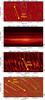 |
Fig. 1 Fragments of the Jovian decametric noise storms of March 14, 2005 (a), b), d)), and March 13, 2004 c). a) Dynamic spectrum containing a sequence of simple quasi linearly drifting S burst (QS). b) Diffuse unstructured L-emission. c) Superposition of S bursts with an apparently distorted band of L emission, with a complex structure including fat bursts separated by shadow (absence of emission) zones. d) Zoomed fragment of the dynamic spectrum contained within the rectangle in a) and illustrating an envelope modulating the occurrence of simple S bursts (MS burst event) is encircled with the green ellipse. Resolution: 1 pixel = 8 kHz × 1.2 ms a), 32 kHz × 4.8 ms b), 12 kHz × 1.2 ms c), and 4 kHz × 0.12 ms d). Yellow segments are plotted just for convenience illustrating the characteristic values of the drift rate. |
In contrast to S emission, L bursts were thought to be devoid of millisecond timescale structures in the time-frequency plane (Carr 1999). Similarly to S bursts, they also occupy a broad frequency band (approximately of the same bandwidth as can be typically occupied by S emission), and are observed either alone or simultaneously with S spectral patterns. In the case of simultaneous occurrence, L and S emissions may overlap in frequency during some time intervals, or otherwise occupy well-separated frequency bands. Observed L burst intensity fluctuates within its spectral range of occurrence at typical timescales of one to several seconds. Such variation has been mainly interpreted as the effect of the interplanetary scintillation, i.e., a modulation arising along the propagation path (Douglas 1967; Genova & Leblanc 1981). A typical pattern of L burst emission is depicted in Fig. 1b where one can see a wideband patch of emission including no apparent short time characteristic structures. The prominent horizontal stripes in Fig. 1b result from the Faraday rotation of the linearly polarized component of the Jovian radio emission (which is 100% elliptically polarized) along the propagation path from Jupiter to the observer (Warwick & Dulk 1964). The major contribution to this frequency-dependent effect comes from the Earth’s ionospheric plasma. As the emission is detected via the UTR-2 antennas, which are only sensitive to the linear (east-west) polarization of the incoming radio waves, bright stripes appear in the dynamic spectrum at frequencies where the received linear wave polarization is parallel to the antennas, and dark stripes where it is perpendicular to the antennas. As the amount of Faraday rotation is proportional to 1/f2 (with f the wave frequency), these Faraday fringes (FF) widen with increasing frequency.
Millisecond radio burst classification and abbreviations used.
The simple classification of decameter radio emissions into only two categories based on the presence or absence of bursts with characteristic timescales on the order of tens of milliseconds became obsolete almost immediately after its introduction. Riihimaa & Carr (1981) noticed that even defining the S bursts by four characteristics (drift rate, very short duration at fixed frequency, small instantaneous bandwidth, and quite short total duration) does not permit them to be distinguished from other complex patterns that occur in dynamic spectra. The improvement of observational facilities, principally the backend spectrometers, which were upgraded from analog filter banks and videotape recorders (Ellis 1973) to semi-digital acousto-optical spectrum analysers (Riihimaa 1975; Ryabov et al. 1997) and digitized videotape (Carr 1999), and then fully digital baseband receivers (Litvinenko et al. 2004; Ryabov et al. 2007, 2010; Koshida et al. 2010), revealed a very complex morphology in the fine structure of Jovian decametric emissions. This led to the introduction of numerous new descriptive types of Jovian decametric radiation, including narrowband (N or NB) emissions (Riihimaa 1985; Boudjada et al. 2000; Oya et al. 2002), fast L bursts (Ellis 1974), L burst lanes (Ellis 1975; Riihimaa 1970, 1978), tilted-V patterns (Riihimaa 1990), S burst trains, “tulip” and “fan” patterns (Riihimaa 1991), fast- (Riihimaa 1991) and slow- (Koshida et al. 2010) drift shadow (FDS and SDS) events, “fat” S bursts (Riihimaa & Carr 1981), and various modulation events (Litvinenko et al. 2009). Most of the above mentioned patterns, can be found in catalogs of Jovian decametric noise storms published by several research teams (Ellis 1979; Flagg et al. 1991; Riihimaa 1992).
Many of these spectral structures can be interpreted as variants of S bursts because of the presence of fast frequency drifts combined with millisecond timescale variability. The necessity of suggesting numerous new types of emission resulted mainly from the lack of vocabulary for describing accurately the extremely complicated burst morphology often observed in dynamic spectra, an example of which is shown in Fig. 1c. This dynamic spectrum combines apparent sequences of comparatively simple S bursts at its top and bottom parts (albeit with different frequency of occurrence), with more complex or fat S bursts in the middle consisting of fast frequency-modulated millisecond patterns of varying bandwidth. Other names such as “distorted L emission” or “fast drift shadows” (Riihimaa 1991) may be more appropriate for describing these structures, since they resemble wideband diffuse L emission distorted by intermittent patches of quenched or enhanced radiation. It is worth mentioning that such a complex dynamic spectrum like the one shown in Fig. 1c is by no means an exception. On the contrary, whenever a long decametric radio noise storm is recorded, it turns out that such complex spectral patterns occupy most of it, whereas simple QS bursts occur intermittently ~10−20% of the time on average (Flagg et al. 1991; Boudjada et al. 1995; Ryabov et al. 1997). If the intrinsic variability of complex S bursts morphologies is neglected, one can accept the simplest classification scheme which roughly divides spectral patterns into simple and complex S bursts: the first class contains QS bursts (such as the brightest and simplest structures shown in Fig. 1a), whereas the latter contains all other more complicated patterns (Carr 1999).
In this paper we attempt to redefine S burst classification based on new observations of several Jovian decametric radio storms recorded between 2004 and 2012 with the new generation of digital receivers (Ryabov et al. 2010) installed at the Ukrainian UTR-2 decameter array (Braude et al. 1978). The large, sensitive, electronically steerable UTR-2 array was combined with a baseband receiver allowing us to record high signal-to-noise ratio waveforms of Jovian radio signals over a broad instantaneous bandwidth (~16 MHz), during continuous time intervals lasting for several hours. As a result, we could trace the evolution of Jovian radio storms at very high resolution from beginning to end. Moreover, as the spectral analysis is computed offline from the waveform recordings, it enables us to vary the time and frequency resolutions of the calculated dynamic spectra, depending on the presence or absence of fine structures. We are thus able to look at the evolution of fine details from different perspectives, i.e., to study their occurrence within much longer or wider spectral patterns. We note that until recently, arbitrary zooming of dynamic spectra in both time and frequency was not possible since the spectrum analysers used had fixed maximum resolutions in frequency, time, or both.
Another advantage of fully digital observations and processing is that we can apply offline interference mitigation algorithms at the pre-processing stage, so that subsequent analysis and classification of spectral patterns is performed on very clean dynamic spectra. This is especially important when different types of spectral patterns with fast and slow frequency drift rates are observed simultaneously within the same frequency band and/or when the calculated dynamic spectrum is severely polluted by interference signals.
We therefore suggest a new classification of Jovian radio bursts based on the different types of time-frequency patterns identified at the highest temporal and spectral resolutions, and on the various frequency drift rates measured in the spectrograms (see Tables 1 and 2).
The analysis of dynamic spectra with zooming possibility reveals new important details of the S burst morphology not reported in previous works (Ellis 1979; Flagg et al. 1991; Riihimaa 1991, 1992; Ryabov et al. 1997). First, we found that even comparatively simple, almost linear frequency drifting QS bursts, can be roughly divided into two groups: one consists of the classical S bursts previously reported in many papers published in this field, and the other related to L emission substructure. To our knowledge, S bursts of the second type have not been discussed elsewhere (although dynamic spectra containing slowly drifting millisecond structures appeared without being described in a previous work, Hess et al. 2009a) and they question the very definition of L bursts as an emission free of spectral structures at timescales shorter than tens to hundreds of milliseconds.
The second observational fact that attracted our attention concerns S bursts that seem to be single solid patterns when observed at relatively low time-frequency resolution, but actually turn out to be composed of a sequence of short linear QS bursts, seemingly triggered or modulated by another fast frequency-drifting process. The short QS bursts that constitute a more complex structure often drift at a slower rate than their modulation envelope defining the burst shape interpreted as a single S burst at lower resolution. The measured frequency drift rate of the envelope can be much steeper than that of its constitutive short QS bursts, sometimes reaching infinite or even positive values. It is likely that the envelope modulation is produced by a physical process different from the one responsible for short or simple linearly drifting bursts. Therefore, it appears necessary to distinguish QS bursts, that can be interpreted in the frame of the quasi-adiabatic motion of keV electron streams moving away from Jupiter (Ellis 1965; Zarka et al. 1996; Hess et al. 2009a), from the apparently more complex modulation or frequency shifting of the whole instantaneous band occupied by simple S bursts. This phenomenon is hereafter called MS for modulated S bursts. As suggested in previous works, the modulation phenomenon may occur either within the source (Willes 2002) or along the propagation path (Shaposhnikov et al. 2011). It should also be noted that S burst modulation has been qualitatively mentioned in papers describing the apparent interaction between S bursts and NB emissions (Riihimaa & Carr 1981; Flagg et al. 1991; Boudjada et al. 2000; Oya et al. 2002).
Finally, we identified fast-drifting, quasi-periodic series of bursts, as events distinct from QS bursts. These bursts are often fat, i.e., have an instantaneous bandwidth and fixed-frequency duration larger than QS bursts. They sometimes appear as shadows cast on background emission; QS bursts can often be seen to emerge sinchronously with these fat or shadowed bursts, called here FS. The association between QS and FS events suggest a physical relationship between their generation processes.
In the following sections, we give a more detailed description of these newly found phenomena, provide illustrative materials for their typical dynamic spectral patterns, and discuss the relevance of several models proposed in the literature that could be used for the interpretation of (at least some of) the observational properties of these various S bursts. Finally, we formulate open questions and outline the framework that can be used for further development of S burst theoretical models.
2. Observational equipment and pre-processing
The decameter radio telescope UTR-2 (Kharkov, Ukraine) (Braude et al. 1978; Abranin et al. 2001) is a phased array of 2040 dipole antennas grouped into two rectangular branches, positioned in the form of the letter T and oriented along the local meridian and parallel, respectively, at coordinates 36°56′E longitude and + 49°38′N latitude. The north-south (NS) branch consists of 1440 basic elements and the east-west (EW) branch contains 600 elements. The telescope has no movable parts, but is electronically steerable by means of a computer controlled time delay phase system, which performs summation in groups of antennas, independently for the EW and NS branches. The array radiation patterns directed at zenith have main lobes of half-maximum extent ~13°×40′ for the EW and ~20′ × 11° for the NS antenna array at 25 MHz. Lowering the observational frequency broadens the lobe width proportionally to frequency difference, whereas deviation from the zenith direction leads to the increase of the beam width, but inversely proportional to the cosine of deviation. The summation of both array branches results in a cross-shaped radiation beam pattern, which has a center spot ~20′ × 40′ directed to the source in zenith direction or somewhat wider in other directions. The basic elements of the array are wide band fat dipoles designed to operate within a band of frequencies between 7 MHz and 32 MHz, thus defining the working band of the whole array.
In 2004−2006, a new digital spectrometer (DRATFA: Decameter Radio Astronomy Time-Frequency Analyser) was developed and installed as the main backend system at the UTR-2 array (Ryabov et al. 2010). In addition to real-time spectral and correlation analysis, the receiver allows direct continuous baseband recording at sampling frequency of ~66 MHz. Initially, waveform recording time was limited by hardware capability to record (~6 s) segments separated by time intervals necessary for swapping the data to hard disk (Ryabov et al. 2007). This shortcoming has been resolved, and since 2007 continuous waveform recording during several hours is feasible.
Sampling is performed in the receiver with 16 bit analog-to-digital conversion (the ADC), ensuring a spurious free dynamic range of 112 dB within the whole band from 0 MHz to 33 MHz. However, in order to avoid the influence of powerful interference signals that may spontaneously occur below 16 MHz during observation and lead to saturation of ADC, a high-pass filter at the receiver input was used. The filter cuts off the low-frequency half of the spectrum (≤16 MHz), ensuring the continuous stable operation of the receiver system any time during observational sessions.
3. Slow S bursts accompanying L emission
The typical dynamic spectrum of a Jovian Io-related emission that can be unambiguously interpreted as L emission is shown in Fig. 1b. However, such a smooth amplitude variation within a wide frequency band is actually quite rarely observed if millisecond scale time resolution is available. The wide emission band is often accompanied by superimposed frequency-drifting structures contradicting the very definition of L bursts as an amorphous diffuse type of emission. Figure 2 shows several examples of dynamic spectra of Jovian decametric L emission actually possessing frequency drifting millisecond structures resembling S bursts. This type of spectral structure is different from the phenomenon of modulation lanes reported in earlier papers (Ellis 1975; Riihimaa 1970, 1978; Imai et al. 1997), since it has a much faster (and typically negative) frequency drift rate in the range of −5 MHz/s to −6 MHz/s, and shorter timescale of amplitude variation at fixed frequency (10−20 ms). These numbers should be compared to ±20 kHz/s to ± 300 kHz/s drift rates in Riihimaa (1978) and 2−10 s timescales in Genova et al. (1981). Somewhat similar although slower drifting modulation lanes (−2 MHz/s) were called “fast lane” (FL) bursts in (Ellis 1975). Although FL bursts with frequency drift about −6 MHz/s also appeared in Fig. 2 of the Ellis paper, it was not said if this kind of emission was typical and often encountered. The −5 MHz/s to −6 MHz/s drift rate, almost constant over the whole decameter band, seems to be the most characteristic property of these emissions, so that we shall refer to this type of emission as LS bursts, short time frequency drifting pulses on L emission background. Spectral structures possessing similar values of the drift rate were reported in Koshida et al. (2010) and called slow drift shadows (SDS), but all their other characteristics are very different from those of LS bursts (SDS consist of much longer (~0.1 s) interruptions of a smooth background and exhibit enhanced edges and slope breaks).
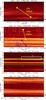 |
Fig. 2 a) Wideband L emission accompanied with frequency drifting LS patterns. b) Simple quasi linear QS bursts intersecting part of the band of LS emission. For example, a deep crossing occurs around 01:27:43,20. This fragment is zoomed from the white rectangle of panel c). c) Wideband L emission accompanied by LS bursts in the band 16−25.5 MHz, simultaneous with QS bursts occurring above ~25 MHz. d) Two powerful sub-bands of LS emissions zoomed from the green rectangle in c). Resolution: 1 pixel = 16 kHz × 2 ms a), 4 kHz × 1 ms b), 28 kHz × 2 ms c), and 8 kHz × 2 ms d). The yellow and blue segments are plotted just for convenience illustrating the characteristic values of the drift rate. |
There are several reasons why we do not interprete LS dynamic spectra such as those shown in Fig. 2a as so-called S burst trains, sequences of S bursts with a high repetition frequency (20−80 Hz) occurring within a limited frequency band (up to ~1 MHz) (Riihimaa 1991). First, the distinctive feature of LS structures is the value of their frequency drift of −5 MHz/s to 6 MHz/s almost independent of frequency, which is much lower than that observed for typical S bursts. Second, the emission occupies a wide frequency band (~8 MHz on Fig. 2a), much larger than the typical bandwidth of S burst trains (generally ~200−500 kHz). Third, the dynamic spectrum shown in Fig. 2a was recorded in a time window located at the edge of a high-probability S bursts occurrence area in the Io phase – CML (central meridian longitude) diagram (see Fig. 2 in Queinnec & Zarka 2001). The CML was about 75°, a value corresponding to L emission preceding an Io-B storm rather than to S emission occurrence.
We note, however, that the last two considerations are not crucial for observing LS bursts. Series of frequency drifting pulses with drift rates of −5 MHz/s to −6 MHz/s repeating at intervals of a few tens of milliseconds can occupy much narrower bandwidth and occur in the middle of a well-developed S burst storm together with usual QS bursts. In such cases, LS emissions are virtually undistinguishable from QS bursts except for their lower frequency drift rate. The difference between the two types of emission becomes evident when both QS and LS bursts coexist within overlapping frequency bands. An example of this situation is depicted in Fig. 2b, where a frequency band centered at ~26 MHz contains QS bursts and it coexists with an LS emission band around ~25 MHz; QS emissions can be recognized by their much faster frequency drift rate of ~−17 MHz/s, whereas the LS bursts drift rate is about −5 MHz/s. Faster drifting QS bursts cross the frequency band occupied by slower LS bursts on several occasions in Fig. 2b.
Figure 2c shows the context of Fig. 2b at lower resolution. The band containing QS bursts occurs simultaneously with apparent L emission at somewhat lower frequency. It is clear from Fig. 2b (which corresponds to the white rectangle in Fig. 2c) that the L emission band contains drifting LS structures, but this phenomenon becomes undetectable in the lower resolution spectrogram depicted as Fig. 2c. Figure 2c thus illustrates that the emission observed in the frequency band ~22 MHz – ~25.5 MHz could be unambiguously identified as L emission in dynamic spectra with moderate time-frequency resolution. Figure 2d shows another view of the same dynamic spectrum (corresponding to the green box in Fig. 2c), where the change in frequency resolution reveals fast intensity modulations in both high intensity frequency sub-bands. The upper one contains obvious LS structures, whereas LS bursts are less pronounced in the lower one and can only be resolved in spectral images with properly tuned resolution. Much weaker emission exists in between the two high intensity sub-bands and below 22 MHz. That weaker emission does not possess any frequency drifting substructure, so that it can be identified as mere L emission.
A last example of LS bursts is given in Fig. 3, where we show a dynamic spectrum containing a narrow band (NB) of emission (~200 kHz bandwidth) containing millisecond substructure. At the resolution of Fig. 3a, one can identify the intense emission band slightly above 16 MHz as NB emission, but the higher resolution of Fig. 3b reveals a train of LS bursts; QS bursts occasionally crossing the LS band are characterized by a much higher drift rate. The simultaneous presence of emissions having two very different drift rates is evident in Fig. 3b (which corresponds to the zoomed green rectangle of Fig. 3a).
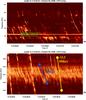 |
Fig. 3 a) Narrow band of LS emission at a frequency slightly below 16.5 MHz, together with complex QS and MS bursts in the band ~14−24 MHz. b) Zoom of the apparent NB emission (inside the rectangle shown in a)) revealing LS emission. The LS structures characterized by a slow frequency drift are occasionally crossed by faster drifting QS bursts. Resolution: 1 pixel = 20 kHz × 2 ms a), and 1 kHz × 0.5 ms b). Blue and yellow segments illustrate drift rates. |
4. Steep drifting bursts actually formed by envelope modulation and shadowing
Flagg & Desch (1979) pointed out a discrepancy between drift rate measurements and the theoretical relation initially proposed by Ellis (1965) that relates the drift rate to the frequency of S bursts (Ellis 1965, 1975; Goldreich 1969; Krausche et al. 1976; Zarka et al. 1996, 1997; Galopeau et al. 1999). The theory explains the quasi linear frequency drift of S bursts by the adiabatic motion of electron beams (or bunches) moving away from Jupiter along the Io flux tube (IFT) and radiating at the local electron gyrofrequency. According to the theory, the drift rate is directly related to the Jovian magnetic field strength variation along the emitting magnetic field lines as well as to the direction and amplitude of the velocity vector of the emitting electrons (i.e., their energy and pitch angle). The model predicts a decline of the drift rate for the frequencies above 30–32 MHz due to electron deceleration close to their magnetic mirror point. Flagg & Desch (1979) measured S bursts drift rates during an Io-B storm at the frequency of 32 MHz using a 500 kHz bandwidth receiver, and derived a much higher value than could be expected from the Ellis model. Zarka et al. (1996) performed a statistical analysis of a significantly larger ensemble of S burst storms at frequencies between 17 MHz and 36 MHz and found that the drift rates averaged over hundreds of individual bursts have a downward trend with frequency, although they demonstrate a huge dispersion of measured drift rates around the mean value at each frequency (solid dots and error bars in Fig. 4). These findings that mainly concern QS bursts were confirmed by Hess et al. (2007a) using a much larger data set at higher time and frequency resolutions.
Measurements from several research groups adapted from Zarka et al. (1997) are summarized in Fig. 4 consistently demonstrating the large dispersion of drift rates measured at frequencies above ~20 MHz. This dispersion is larger than uncertainties resulting from the algorithms estimating the drift rates from dynamic spectra even in the presence of interference signals, thus it must have a physical cause, that has not yet been discovered. We suggest that some of the variations in the drift rates measured from storm to storm and even from one time interval to another within the same storm might result from the mixing of bursts generated by several different physical mechanisms.
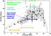 |
Fig. 4 Comparison of the Ellis drift rate model for S bursts (lines) to various measurements from different research groups (open and solid circles), adapted from Fig. 2 of Zarka et al. (1997). The lines were calculated assuming adiabatically moving streams of electrons at the speed of v = 0.14c (dashed) and v = 0.14 ± 0.03c (dotted), with an equatorial pitch angle of 2.8°. We superimposed four horizontal bars indicating typical drift rates of the different types of millisecond bursts discussed in the text. From top to bottom, we find the modulated S bursts envelopes (MS bursts), the fast drift (FS) events, the simple QS bursts, and the slower LS bursts. The position of each bar was calculated as an average over measured values within a representative but arbitrarily selected dynamic spectrum of duration ~3 s. Measurements performed at other times may show considerable variability. For example, in Fig. 1c apparent QS bursts above 23.5 MHz have drift rates up to ~27 MHz/s (although it may also be a variant of MS emission). |
The existence of several superimposed, coexisting, or competing processes defining the time-frequency shape of individual bursts is strongly suggested by the examination of dynamic spectra calculated at high time and frequency resolutions, because they reveal simultaneous, superimposed spectral patterns. The simplest one that initially attracted attention to this kind of Jovian decametric radiation is QS bursts, initially called simply S bursts. Low resolution dynamic spectra (δf = 13 kHz and δt = 10 ms in Zarka et al. 1996) did not allow the investigation of the sub-structures in S bursts, but high resolution spectral images reveal at least two other characteristic patterns with very different morphologies. The first one, MS, appears to be caused by the rapid frequency modulation of the envelope of S bursts, over a wide frequency band. It should be also noted that MS, modulated S bursts envelope, was also referred to as “undulations” in previous works (Flagg et al. 1991). The second pattern is closely related to the FDS events of (Riihimaa 1991), and it is also often accompanied by QS bursts, detectable only through high resolution time-frequency analysis. Although both of these classes of emission have already been discussed in previous works, they were not interpreted as generated by physical processes different from those producing the simple QS bursts. We document this hypothesis below.
4.1. Modulated S burst envelopes
Several cases of complex time-frequency patterns called “undulating emission bands” have been discussed in Riihimaa & Carr (1981); Riihimaa (1990); Flagg et al. (1991); Boudjada et al. (2000); Oya et al. (2002); Litvinenko et al. (2009). The phenomenon consists in fast perturbations in a band of decametric emission that can form very complicated shapes in the time-frequency plane. The original (unperturbed) emission is often confined to a narrow range of frequencies (hundreds of kHz in bandwidth, similar to NB emission), but can sometimes cover a band up to several MHz. The dynamic spectra in the presence of this frequency modulation process show erratic frequency shifts of the whole emission band at tens of milliseconds timescale, with an amplitude comparable to or larger than its overall bandwidth, as well as sporadic quenching of the emission in part of the band. Both L emission and S burst trains can be affected by this modulation phenomenon. The resulting patterns may look like S bursts at moderate time-frequency resolution.
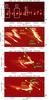 |
Fig. 5 Sequence of modulated S bursts envelope (MS). a) The fragments denoted by b), c), and d) are zoomed in the corresponding panels of the figure. The remarkable feature is the presence of two apparent frequency drift rates: one for the envelope, and another one for elementary quasi linear QS bursts contained in or emerging from this envelope. The green lines in b)–d) delineate the slope of the envelope, whereas the yellow ones are drawn approximately parallel to the average slope of QS bursts inside the envelope. We note the presence of a positive drift of the envelope in d) that would be interpreted as a positively drifting S burst in a lower resolution image such as a). Resolution: 1 pixel = 16 kHz × 2 ms a), 4 kHz × 0.1 ms b), 8 kHz × 0.2 ms c), and 8 kHz × 0.2 ms d). |
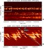 |
Fig. 6 a) Modulated S bursts in the band of decametric emission between 25 MHz and 29 MHz. The rectangular area is zoomed in b). The high resolution image in b) reveals the emergence (forking) from the wide band emission of sporadic narrowband QS bursts with characteristic instantaneous bandwidth of 5−10 kHz (encircled). Resolution: 1 pixel = 32 kHz × 2 ms a), and 8 kHz × 0.4 ms b). The blue segment illustrates the drift rate. |
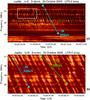 |
Fig. 7 a) Fast drifting quasi-periodic “fat” S events (FS) with a negative drift rate ~-30 MHz/s. The rectangular area is zoomed in b). The high resolution image in b) reveals superimposed or forking QS bursts (encircled) with their usual drift rate ~-17 MHz/s and bandwidth ~10 kHz. Resolution: 1 pixel = 32 kHz × 2 ms a), 8 kHz × 0.5 ms b). Blue and green segments illustrate drift rates. |
In Fig. 5a we plot a fragment of the Io-B storm of October 30, 2008, that presents a sequence of complex S bursts caused by envelope modulation, that we will call hereafter MS bursts. The modulated nature of these bursts becomes evident only at higher resolution as shown in Panels b−d of Fig. 5, which contain zoomed fragments of the dynamic spectrum in Fig. 5a. It turns out that the millisecond patterns that look like typical S bursts at a lower resolution reveal an internal structure composed of series of QS bursts. It is possible that this mechanism is also responsible for the pattern shown in Fig. 1d. There, the encircled event is clearly of a different nature than elementary QS bursts, being composed of a series of short QS bursts possessing frequency drift rates smaller than their envelope. Figure 6 is another example of MS emission within a wide band of decametric radiation (~4 MHz). A blow-up of the fragment in the white rectangle of Fig. 6a is shown in Fig. 6b, presenting narrowband frequency drifting structures that may be caused by a modulation process similar to the one operating in Fig. 1d. In Fig. 6b, emergence of QS bursts is visible at the lower edge of the wider emission band, leaving uniform the upper part of the emission band. The whole band containing the radiation seems to be strongly perturbed (modulated) by a specific process generating its envelope. This type of structure was also referred to as fast drift shadows (Riihimaa 1991) or tilted V events (Riihimaa 1990).
There are at least two promising models in the literature that can be used to explain such fast frequency modulations of the Jupiter decametric emission. Willes (2002) proposed that phase bunching can be a universal mechanism for generating fine structures in dynamic spectra, such as S bursts. It remains an open question whether this model can be used to explain all types of observed S burst morphology, but it seems well adapted to MS events. In the framework of the Willes model, radio waves can be amplified within a limited interaction area located along the IFT, where the phase bunching effect occurs. This interaction area can move up and down along the magnetic field lines, thus causing frequency modulation of the emission generated at the local gyrofrequency, i.e., creating an oscillating envelope.
Another model capable of producing frequency modulation suggests that a severe distortion of the envelope of the emission can occur near its source because of wave propagation effects through the magnetized plasma (Shaposhnikov et al. 2011). If the magnetic field perturbation (e.g., due to Alfvén waves) is large enough and the ambient plasma is sufficiently dense, the resulting dynamic spectral patterns of S emission can have a shape very similar to MS events. It appears unlikely, however, that this model can apply universally to all types of S burst patterns, including QS, QS forking from MS, or FS events.
Finally, another model mixing Alfvén waves and radio propagation effects is discussed in a series of papers by Arkhypov & Rucker (see, e.g., Arkhypov & Rucker 2012, and references therein), but it incorporates many ad hoc assumptions not supported by observations and does not convincingly explain the observed features.
4.2. Fast drifting S events
Wideband decameter bursts extending across a frequency band of 10 MHz or more and recurring at a rate of 20−40 s-1 have been described in Riihimaa (1991, 1992) after a time-frequency resolution of 7 ms × 70 kHz was reached with an acousto-optical spectrometer installed at the Aarne Karjalainen Observatory (Finland). These bursts were named fast drift shadow S events (FDS-S), since they incorporated features resembling both FDS (such as in Fig. 6b, but over a broader bandwidth) and S bursts. They appear as fast frequency drifting stripes alternating quenched and enhanced emission. Although often quasi-periodic, their time profile is different from fringes that could be produced e.g., by diffraction. The initial name FDS-S is unnecessarily complicated, as there is no FDS-L type of Jovian emission known, and the description of alternating stripes by both shadowing and enhanced bursts seems redundant. We will thus simply refer to these bursts as FS (fast S bursts) because of their unusually high drift rates, typically −30 MHz/s or steeper and because they show little dependence on the frequency. These events can occur quasi-periodically, or sporadically when the periodicity is disrupted by envelope modulation arising inside the band covered by the emission (leading to MS patterns). The instantaneous bandwidth or fixed-frequency duration of individual FS is larger than that of QS bursts, which explains why they were sometimes referred to as fat S bursts (Riihimaa & Carr 1981).
Zooming in on dynamic spectra containing FS emission reveals new details. It appears that QS bursts with slower frequency drift rates and narrow bandwidths, often accompany FS emissions. In Fig. 7b, they seem to fork out from FS bursts sporadically at various locations in the dynamic spectrum (see encircled details). This suggests a physical association, but at the same time their different characteristics may be due to distinct, possibly interacting generation processes.
Hess et al. (2007b) suggested that the keV electrons producing the Jovian S bursts via the cyclotron maser instability (CMI) can be accelerated by trains of Alfvén waves coming from a resonator located slightly above Jupiter’s ionosphere, between the ionospheric conductive layer and the peak in Alfvén speed at ~0.1 Jovian radius above it (Ergun 2006). Computer simulations of electron acceleration by the Alfvén waves showed that periodic electron beams can generate radio emissions with characteristics very similar to those of the FS emission. This mechanism is thus promising for explaining Jovian millisecond bursts of this type (see e.g., Fig. 1 of Hess et al. 2009b).
5. Conclusions and discussion
We presented an analysis of dynamic spectra of Jovian decametric emissions computed with arbitrarily high time and frequency resolutions. This was achieved due to the use of a baseband digital receiver capable of continuous waveform signal recording at a sampling rate of 66 MHz during several hours, i.e., long enough for recording the entire development of Jovian radio noise storms. High resolution dynamic spectra revealed spectral patterns unresolved in previous studies and allowed us to revise the description of Jupiter’s millisecond S bursts in a spirit of simplification and clarification.
The simplest narrowband (5−10 kHz) S bursts are simply renamed QS bursts (quasi linear S bursts). They always have a negative drift rate, between −15 MHz/s and −20 MHz/s in the frequency range of UTR-2 (see Fig. 4). Their frequency drift rates were demonstrated to be consistent with the model of CMI emission by keV electrons in quasi-adiabatic motion along Io-Jupiter magnetic field lines, and even their observed slope breaks can be explained by magnetic field aligned electric potential drops along the IFT (Hess et al. 2007a, 2009a,b). Alfvén waves can play a central role in electron acceleration (Hess et al. 2007b), but the exact scenario of acceleration of the electron populations that emit non-periodic isolated QS bursts (via the CMI) is not yet fully understood.
More complex S bursts appear in our classification as (i) the result of a process modulating the envelope of QS bursts or (ii) trains of fast drifting stripes alternating quenched and enhanced emission. We named the former MS (modulated S bursts) and the latter FS (fast-drifting S bursts) emission.
Modulated envelope S emissions includes an additional level of complexity relative to QS bursts. They are characterized by two distinct frequency drift rates, one corresponding to elementary QS bursts contained in the modulated envelope, with their usual drift rates, and another characterizing the envelope itself (cf. for example Figs. 1a and d). This detailed structure is discernible only at high time and frequency resolutions. At moderate resolutions, MS bursts look like long solid narrowband lines without distinguishable sub-bursts. They are assimilated to their envelope, that can show any value of the drift rate, including very steep negative or (rarely) positive values. We suggest that this phenomenon is entirely responsible for S bursts reported with apparent abnormally steep or positive drift rates, which is actually that of the emission envelope. Two models are mentioned in Sect. 4.1 that could account for the MS phenomenon, one being related to the emission process in the source (phase bunching; Willes 2002), the second invoking perturbations imposed on the wave propagation by the perturbed magnetized plasma in/near the source (Shaposhnikov et al. 2011).
Fast drift shadow emission is generally associated with Io-B noise storms, and it is characterized by unusually high negative frequency drift rates (compared to QS bursts and the Ellis model with keV electrons) and frequent quasi-periodicity of the fast drifting structures. This quasi-periodicity can be explained by CMI emission of electrons accelerated by Alfvén wave trains (Hess et al. 2007b, 2009b). However, abnormally steep drift rates of FS emissions would imply high energy electrons (~3 times that of QS bursts, i.e., 10−15 keV) in the framework of a cyclotron maser-based model. The origin of these electrons, the constancy of their energy, and the fat character of FS emission is not understood. If the stripes of quenched emission are considered as a result of shadowing effect (which is also present in MS emission; see Fig. 6b), then a possible explanation has been proposed by Gopalswamy (1986) that invokes CMI absorption of L emission in presence of S electrons (which could also account for the enhanced stripes).
For both MS and FS emissions, emergence of narrowband QS bursts from smoother emission of broader bandwidth that we have named the forking process is often observed. In the case of MS emission, forking often occurs at the lower frequency edge of MS patterns (Fig. 6b). In the case of FS emission, forking seems to occur on both sides of fast drifting stripes (Fig. 7b). This phenomenon seems to imply both related and distinct generation processes for QS bursts and MS or FS patterns. Although we do not yet have any theoretical explanation for it, we can simply notice that emergence of fine substructures from a broader emission pattern is known for solar Type II radio bursts, the emerging or forking structures being called “herringbones” (Bougeret et al. 1998). In that case, accelerated electrons are thought to be produced in both directions from a shock moving away from the Sun through the solar corona and wind. A similar model transposed to Jovian S bursts could suggest accelerated electrons produced in both directions from an interaction region such as in Willes (2002).
Finally, a possible link between L and S emissions was found in the form of slowly drifting narrowband LS patterns inside of bands of L emission. L emission can be accounted for by the CMI operating in large scale depleted sources (Mottez et al. 2010). However, this theory does not explain the structure detected in the LS emission, and future work is required to determine its source.
As seen above, several successful or promising models exist that can explain some of the observed features, but many others still lack a convincing theoretical interpretation. Even for the simplest QS burst, consistent with the CMI theory and Ellis model, features such as the overall bandwidth (and consequently overall duration) of each burst as well as their instantaneous bandwidth and fixed-frequency duration are not clearly explained. They may be related to the interval along a Io-Jupiter field line, along which an unstable electron distribution exists, and the instantaneous spatial extent of this electron distribution. Less understood is the fact that S or L emission sometimes occur within well-defined frequency bands experiencing slow drift in frequency. Sometimes several such bands exist simultaneously on dynamic spectra. They can experience frequency merging or splitting at timescales from tens of seconds to several minutes (Leblanc & Rubio 1982), and their bandwidths can range from a hundred kHz to ≥10 MHz. What defines the bandwidth extent and its time variations remains an open problem. A phenomenological interpretation in terms of moving bulbs along the IFT had been proposed in Ryabov (1994), but it did not receive a wide acceptance.
There is thus still room for developing the theoretical frame of the fine structures of Jovian radio emissions that may relate to other astrophysical structured radio emissions. In addition to the now well-accepted CMI and Ellis model, other theories have been proposed for interpreting QS bursts (see e.g., Zarka 1998). One of them involves the disruption of current filaments (carried by Alfvén waves) along the IFT (Ryabov 1994). Although not accepted as a standalone interpretation of QS bursts, it might be a useful additional ingredient to the theory based on CMI and the Ellis model. A new theory was recently proposed for the generation of fine structures in the Earth’s auroral kilometric radiation (AKR) from CMI in electron holes (EH) in the upward current region above the auroras by Treumann et al. (2011). This theory explains in an elegant way the production (on the oblique R-X mode) of narrowband radio emission significantly above the local cyclotron frequency, but suffering problems of growth rate. It was adapted in (Treumann et al. 2012) to the case of EH in the downward current region, where higher densities lead to larger growth rates and possible radiation escape into both the downward and upward current regions. This theory is very promising for an application to the case of Jupiter, as magnetic field-aligned electric potential drops (Hess et al. 2007a) and probably also electron and ion holes (Hess et al. 2009b) do exist and move (Hess et al. 2009a) along the IFT. Further discussion is beyond the scope of this paper.
Table 2 attempts a first synthesis of the above discussion by listing all patterns observed in the dynamic spectra displayed in Figs. 1–7 of the present paper, which are a representative sample of all types of fine structures of the Jovian decameter emission. For each structure, we list observed characteristics − in particular the drift rate – and a possible generation mechanism (in a purely qualitative and indicative way). We believe that QS, MS, FS, LS, and forking altogether cover all the varieties of very complex shapes that can be identified in spectrograms of Jovian emission at millisecond – kHz resolutions. Higher time and/or frequency resolution images can be numerically obtained, but they seem to carry no sensible additional information as can be expected from the fundamental limit of Fourier analysis Δf × Δτ ≅ 1.
Phenomenology is important at several stages of the study of complex phenomena. At pioneering stages, ad hoc names were invented as new structures were discovered in dynamic spectra (as done in the papers by Riihimaa), but they did not necessarily correspond to distinct or identified physical phenomena. With the recent (albeit still very incomplete) theoretical developments of planetary auroral and radio emission physics, we believe that a redefinition, simplification, and synthesis of the phenomenology is necessary to set a proper frame for future physical studies. These studies should experience new significant developments with the in situ exploration of Jovian radio sources by JUNO (≥20161) and then by JUICE (≥2020−25), down to very low frequencies. In parallel, new ground-based facilities such as LOFAR (van Haarlem et al. 2013) and NenuFAR (Zarka et al. 2012) should permit high sensitivity, high angular, spectral, and temporal resolutions studies of the Jovian decameter emission up to its highest frequency (~40 MHz).
References
- Abranin, E. P., Bruck, Yu. M., Zakharenko, V. V., et al. 2001, Exp. Astron., 11, 85 [NASA ADS] [CrossRef] [Google Scholar]
- Arkhypov, O. V., & Rucker, H. O. 2012, Icarus, 220, 216 [NASA ADS] [CrossRef] [Google Scholar]
- Boudjada, M. Y., Rucker, H. O., Ladreiter, H. P., & Ryabov, B. P. 1995, A&A, 295, 782 [NASA ADS] [Google Scholar]
- Boudjada, M.Y., Galopeau, P. H. M., Rucker, H. O., & Lecacheux, A. 2000, A&A, 363, 316 [NASA ADS] [Google Scholar]
- Bougeret, J.-L., Zarka, P., Caroubalos, C., et al. 1998, GRL, 25, 2513 [Google Scholar]
- Braude, S. Ya., Megn, A. V., Ryabov, B. P. et al. 1978, Astrophys. Space Sci., 54, 3 [NASA ADS] [CrossRef] [Google Scholar]
- Carr, T. D., & Reyes, F. 1999, JGR, 104, 25127 [Google Scholar]
- Douglas, J. N., & Smith, H. J. 1967, ApJ, 148, 885 [Google Scholar]
- Ellis, G. R. A. 1962, Aust. J. Phys., 15, 344 [NASA ADS] [CrossRef] [Google Scholar]
- Ellis, G. R. A. 1965, Radio Sci., 69D, 1513 [NASA ADS] [Google Scholar]
- Ellis, G. R. A. 1973, Aust. J. Phys., 26, 253 [NASA ADS] [CrossRef] [Google Scholar]
- Ellis, G. R. A. 1974, Proc. ASA, 5, 236 [NASA ADS] [Google Scholar]
- Ellis, G. R. A. 1975, Nature, 253, 415 [NASA ADS] [CrossRef] [Google Scholar]
- Ellis, G. R.A. 1979, An atlas of selected spectra of the Jupiter S-bursts (Physics Dept., Univ. of Tasmania) [Google Scholar]
- Ergun, R. E., Su, Y.-J.,Andersson, L., et al. 2006, JGR, 111, A06212 [Google Scholar]
- Flagg, R. S., & Desch, M. D. 1979, JGR, 84, 4238 [Google Scholar]
- Flagg, R. S., Greenman, W. G., Reyes, F., & Carr, T. D. 1991, A catalog of high resolution Jovian decametric radio noise burst spectra (Univ. of Florida, Gainesville) [Google Scholar]
- Gallet, R. M. 1961, in Planets and Satellites, eds. G. P. Kuiper, & B. M. Middlehurst (Chicago: Univ. of Chicago Press) [Google Scholar]
- Galopeau, P. H. M., Boudjada, M. Y., & Rucker, H. O. 1999, A&A, 341, 918 [NASA ADS] [Google Scholar]
- Genova, F., & Leblanc, Y. 1981, A&A, 98, 133 [NASA ADS] [Google Scholar]
- Genova, F., Aubier, M. G., & Lecacheux, A. 1981, A&A, 104, 229 [NASA ADS] [Google Scholar]
- Goldreich, P., & Lynden-Bell, D. 1969, ApJ, 156, 59 [NASA ADS] [CrossRef] [Google Scholar]
- Gopalswamy, N. 1986, Earth Moon Planets, 35, 93 [NASA ADS] [CrossRef] [Google Scholar]
- Hess, S., Zarka, P., & Mottez, F. 2007a, Planet. Space Sci., 55, 89 [NASA ADS] [CrossRef] [Google Scholar]
- Hess, S., Mottez, F., & Zarka, P. 2007b, JGR, 112, A11212 [NASA ADS] [CrossRef] [Google Scholar]
- Hess, S., Zarka, P., Mottez, F., & Ryabov, V. B. 2009a, Planet. Space Sci., 57, 23 [NASA ADS] [CrossRef] [Google Scholar]
- Hess, S., Mottez, F., & Zarka, P. 2009b, GRL, 36, L14101 [Google Scholar]
- Imai, K., Wang, L., & Carr, T. D. 1997, JGR, 102, 7127 [Google Scholar]
- Koshida, T., Ono, T., Iizima, M., & Kumamoto, A. 2010, JGR, 115, A01202 [NASA ADS] [CrossRef] [Google Scholar]
- Krausche, D. S., Flagg, R. S., Lebo, G. R., & Smith, A. G. 1976, Icarus, 29, 463 [NASA ADS] [CrossRef] [Google Scholar]
- Leblanc, Y., & Rubio, M. 1982, A&A, 111, 284 [NASA ADS] [Google Scholar]
- Litvinenko, G. V., Rucker, H. O., Vinogradov, V. V., et al. 2004, A&A, 426, 343 [NASA ADS] [CrossRef] [EDP Sciences] [Google Scholar]
- Litvinenko, G.V., Lecacheux, A., Rucker, H. O., et al. 2009, A&A, 493, 651 [NASA ADS] [CrossRef] [EDP Sciences] [Google Scholar]
- Mottez, F., Hess, S., & Zarka, P. 2010, Planet. Space Sci., 58, 1414 [NASA ADS] [CrossRef] [Google Scholar]
- Oya, M., Oya, H., Ono, T., & Iizima, M. 2002, Earth, Moon Planets, 88, 187 [CrossRef] [Google Scholar]
- Queinnec, J., & Zarka, P. 2001, Planet. Space Sci., 49, 365 [NASA ADS] [CrossRef] [Google Scholar]
- Riihimaa, J. J. 1970, A&A, 4, 180 [NASA ADS] [Google Scholar]
- Riihimaa, J. J. 1975, A&A, 39, 69 [NASA ADS] [Google Scholar]
- Riihimaa, J. J. 1978, Astrophys. Space Sci., 56, 503 [Google Scholar]
- Riihimaa, J. J. 1985, Earth, Moon, Planets, 32, 9 [Google Scholar]
- Riihimaa, J. J. 1990, Earth, Moon, Planets, 48, 49 [Google Scholar]
- Riihimaa, J. J. 1991, Earth, Moon, Planets, 53, 157 [Google Scholar]
- Riihimaa J. J. 1992, Wide-range high-resolution S-burst spectra of Jupiter (Finland: Univ. of Oulu) [Google Scholar]
- Riihimaa, J. J., & Carr, T. D. 1981, The Moon and the Planets, 25, 373 [NASA ADS] [CrossRef] [Google Scholar]
- Ryabov, B. P. 1994, JGR, 99, 8441 [Google Scholar]
- Ryabov, B. P., & Gerasimova, N. N. 1990, Sporadic radio emissions of Jupiter at decameter wavelength (Kiev: Naukova Dumka) (in Russian) [Google Scholar]
- Ryabov, B. P., Zarka, P., Rucker, H. O., et al. 1997, Recurrent fine structures in Jovian S-burst emission, in Planetary Radio Emissions IV, eds. H. O. Rucker, W. S. Kurth, P. Louarn, & G. Fischer (Vienna: Austrian Academy of Sciences Press), 65 [Google Scholar]
- Ryabov, V. B., Ryabov, B. P., Vavriv, D. M., et al. 2007, JGR, 112, A09206 [Google Scholar]
- Ryabov, V. B., Vavriv, D. M., Zarka, P., et al. 2010, A&A, 510, A16 [NASA ADS] [CrossRef] [EDP Sciences] [Google Scholar]
- Shaposhnikov, V. E., Korobkov, S. V., Rucker, H. O., et al. 2011, JGR, 116, A03205 [NASA ADS] [CrossRef] [Google Scholar]
- Treumann, R. A., Baumjohann, W., & Pottelette, R. 2011, Ann. Geophys., 29, 1885 [NASA ADS] [CrossRef] [Google Scholar]
- Treumann, R. A., Baumjohann, W., & Pottelette, R. 2012, Ann. Geophys., 30, 119 [NASA ADS] [CrossRef] [Google Scholar]
- van Haarlem, M. P., Wise, M. W., Gunst, A. W., et al. 2013, A&A, 556, A2 [NASA ADS] [CrossRef] [EDP Sciences] [Google Scholar]
- Warwick, J. W., & Dulk, G. A. 1964, Science, 145, 380 [NASA ADS] [CrossRef] [Google Scholar]
- Willes, A. J. 2002, ApJ, 107, 1061 [Google Scholar]
- Zarka, P. 1998, JGR, 103, 20159 [CrossRef] [Google Scholar]
- Zarka, P., Farges, T., Ryabov, B. P., Abada-Simon, M., & Denis, L. 1996, GRL, 23, 125 [CrossRef] [Google Scholar]
- Zarka, P., Ryabov, B. P., Ryabov, V. B., et al. 1997, in Planetary Radio Emissions IV, eds. H. O. Rucker et al. (Vienna: Austrian Academy of Sciences Press), 51 [Google Scholar]
- Zarka, P., Girard, J. N., Tagger, M., Denis, L., & the LSS team 2012, Proc. SF2A, eds. S. Boissier et al. (CNRS), 687 [Google Scholar]
All Tables
All Figures
|
Fig. 1 Fragments of the Jovian decametric noise storms of March 14, 2005 (a), b), d)), and March 13, 2004 c). a) Dynamic spectrum containing a sequence of simple quasi linearly drifting S burst (QS). b) Diffuse unstructured L-emission. c) Superposition of S bursts with an apparently distorted band of L emission, with a complex structure including fat bursts separated by shadow (absence of emission) zones. d) Zoomed fragment of the dynamic spectrum contained within the rectangle in a) and illustrating an envelope modulating the occurrence of simple S bursts (MS burst event) is encircled with the green ellipse. Resolution: 1 pixel = 8 kHz × 1.2 ms a), 32 kHz × 4.8 ms b), 12 kHz × 1.2 ms c), and 4 kHz × 0.12 ms d). Yellow segments are plotted just for convenience illustrating the characteristic values of the drift rate. |
| In the text | |
|
Fig. 2 a) Wideband L emission accompanied with frequency drifting LS patterns. b) Simple quasi linear QS bursts intersecting part of the band of LS emission. For example, a deep crossing occurs around 01:27:43,20. This fragment is zoomed from the white rectangle of panel c). c) Wideband L emission accompanied by LS bursts in the band 16−25.5 MHz, simultaneous with QS bursts occurring above ~25 MHz. d) Two powerful sub-bands of LS emissions zoomed from the green rectangle in c). Resolution: 1 pixel = 16 kHz × 2 ms a), 4 kHz × 1 ms b), 28 kHz × 2 ms c), and 8 kHz × 2 ms d). The yellow and blue segments are plotted just for convenience illustrating the characteristic values of the drift rate. |
| In the text | |
|
Fig. 3 a) Narrow band of LS emission at a frequency slightly below 16.5 MHz, together with complex QS and MS bursts in the band ~14−24 MHz. b) Zoom of the apparent NB emission (inside the rectangle shown in a)) revealing LS emission. The LS structures characterized by a slow frequency drift are occasionally crossed by faster drifting QS bursts. Resolution: 1 pixel = 20 kHz × 2 ms a), and 1 kHz × 0.5 ms b). Blue and yellow segments illustrate drift rates. |
| In the text | |
|
Fig. 4 Comparison of the Ellis drift rate model for S bursts (lines) to various measurements from different research groups (open and solid circles), adapted from Fig. 2 of Zarka et al. (1997). The lines were calculated assuming adiabatically moving streams of electrons at the speed of v = 0.14c (dashed) and v = 0.14 ± 0.03c (dotted), with an equatorial pitch angle of 2.8°. We superimposed four horizontal bars indicating typical drift rates of the different types of millisecond bursts discussed in the text. From top to bottom, we find the modulated S bursts envelopes (MS bursts), the fast drift (FS) events, the simple QS bursts, and the slower LS bursts. The position of each bar was calculated as an average over measured values within a representative but arbitrarily selected dynamic spectrum of duration ~3 s. Measurements performed at other times may show considerable variability. For example, in Fig. 1c apparent QS bursts above 23.5 MHz have drift rates up to ~27 MHz/s (although it may also be a variant of MS emission). |
| In the text | |
|
Fig. 5 Sequence of modulated S bursts envelope (MS). a) The fragments denoted by b), c), and d) are zoomed in the corresponding panels of the figure. The remarkable feature is the presence of two apparent frequency drift rates: one for the envelope, and another one for elementary quasi linear QS bursts contained in or emerging from this envelope. The green lines in b)–d) delineate the slope of the envelope, whereas the yellow ones are drawn approximately parallel to the average slope of QS bursts inside the envelope. We note the presence of a positive drift of the envelope in d) that would be interpreted as a positively drifting S burst in a lower resolution image such as a). Resolution: 1 pixel = 16 kHz × 2 ms a), 4 kHz × 0.1 ms b), 8 kHz × 0.2 ms c), and 8 kHz × 0.2 ms d). |
| In the text | |
|
Fig. 6 a) Modulated S bursts in the band of decametric emission between 25 MHz and 29 MHz. The rectangular area is zoomed in b). The high resolution image in b) reveals the emergence (forking) from the wide band emission of sporadic narrowband QS bursts with characteristic instantaneous bandwidth of 5−10 kHz (encircled). Resolution: 1 pixel = 32 kHz × 2 ms a), and 8 kHz × 0.4 ms b). The blue segment illustrates the drift rate. |
| In the text | |
|
Fig. 7 a) Fast drifting quasi-periodic “fat” S events (FS) with a negative drift rate ~-30 MHz/s. The rectangular area is zoomed in b). The high resolution image in b) reveals superimposed or forking QS bursts (encircled) with their usual drift rate ~-17 MHz/s and bandwidth ~10 kHz. Resolution: 1 pixel = 32 kHz × 2 ms a), 8 kHz × 0.5 ms b). Blue and green segments illustrate drift rates. |
| In the text | |
Current usage metrics show cumulative count of Article Views (full-text article views including HTML views, PDF and ePub downloads, according to the available data) and Abstracts Views on Vision4Press platform.
Data correspond to usage on the plateform after 2015. The current usage metrics is available 48-96 hours after online publication and is updated daily on week days.
Initial download of the metrics may take a while.