| Issue |
A&A
Volume 567, July 2014
|
|
|---|---|---|
| Article Number | A76 | |
| Number of page(s) | 32 | |
| Section | Extragalactic astronomy | |
| DOI | https://doi.org/10.1051/0004-6361/201423906 | |
| Published online | 14 July 2014 | |
The radio-loud AGN population at z ≳ 1 in the COSMOS field
I. selection and spectral energy distributions⋆
1 SISSA-ISAS, via Bonomea 265, 34136 Trieste, Italy
e-mail: This email address is being protected from spambots. You need JavaScript enabled to view it.
2 Physics Department, The Technion, 32000 Haifa, Israel
3 Physics Department, Faculty of Natural Sciences, University of Haifa, 31905 Haifa, Israel
4 INAF − Osservatorio Astrofisico di Torino, Strada Osservatorio 20, 10025 Pino Torinese, Italy
5 Space Telescope Science Institute, 3700 San Martin Drive, Baltimore, MD 21218, USA
6 INAF-Istituto di Radio Astronomia, via P. Gobetti 101, 40129 Bologna, Italy
7 Center for Astrophysical Sciences, Johns Hopkins University, 3400 N. Charles Street Baltimore, MD 21218, USA
8 INAF-Osservatorio Astronomico di Brera, via E. Bianchi 46, 23807 Merate, Italy
9 INFN- Sezione di Trieste, via Valerio 2, 34127 Trieste, Italy
Received: 30 March 2014
Accepted: 6 May 2014
Abstract
We select a sample of radio galaxies at high redshifts (z ≳ 1) in the COSMOS field by cross-matching optical and infrared (IR) images with the FIRST radio data. The aim of this study is to explore the high-z radio-loud (RL) active galactic nuclei (AGN) population at much lower luminosities than the classical samples of distant radio sources, which are similar to those of the local population of radio galaxies. Precisely, we extended a previous analysis focused on low-luminosity radio galaxies. The wide multiwavelength coverage provided by the COSMOS survey allows us to derive their spectral energy distributions (SEDs). We model them with our own developed technique 2SPD that includes old and young stellar populations and dust emission. When added to those previously selected, we obtain a sample of 74 RL AGN. The SED modeling returns several important quantities associated with the AGN and host properties. The resulting photometric redshifts range from z ~ 0.7 to 3. The sample mostly includes compact radio sources but also 21 FR IIs sources; the radio power distribution of the sample covers ~1031.5 − 1034.3 erg s-1 Hz-1, thus straddling the local FR I/FR II break. The inferred range of stellar mass of the hosts is ~1010 − 1011.5M⊙. The SEDs are dominated by the contribution from an old stellar population with an age of ~1 − 3 Gyr for most of the sources. However, UV and mid-IR (MIR) excesses are observed for half of the sample. The dust luminosities inferred from the MIR excesses are in the range, Ldust ~ 1043 − 1045.5 erg s-1, which are associated with temperatures approximately of 350−1200 K. Estimates of the UV component yield values of ~1041.5 − 1045.5 erg s-1 at 2000 Å. The UV emission is significantly correlated with both IR and radio luminosities; the former being the stronger link. However, the origin of UV and dust emission, whether it is produced by the AGN of by star formation, is still unclear. Our results show that this RL AGN population at high redshifts displays a wide variety of properties. Low-power radio galaxies, which are associated with UV- and IR-faint hosts are generally similar to red massive galaxies of the local FR Is. At the opposite side of the radio luminosity distribution, large MIR and UV excesses are observed in objects consistent with quasar-like AGN, as also proved by their high dust temperatures, which are more similar to local FR IIs.
Key words: galaxies: active / galaxies: high-redshift / galaxies: jets / galaxies: nuclei / galaxies: photometry
Appendix A is available in electronic form at http://www.aanda.org
© ESO, 2014
1. Introduction
The advent of a multiband dataset from large area surveys marked the starting point of a new scientific approach based on large samples of sources through a multiwavelength analysis. The immense number of sources and the completeness of the sample is fundamental for obtaining results with high statistical foundations. Clear examples are represented by large surveys, such as Sloan Digital Sky Survey (SDSS; York et al. 2000) and COSMOS (Scoville et al. 2007), which provide wide multiwavelength coverage. The association of targets at different wavelengths helps us to determine the properties of the sources and, especially, to derive their SEDs.
Among the most energetic phenomena in the Universe, radio galaxies occupy an important position in the study of the fundamental issues of modern astrophysics, such as accretion onto black holes (BH), the co-evolution between the host galaxy and BH, and the feedback process of the active galactic nucleus (AGN) on the interstellar and intercluster medium (e.g. Hopkins et al. 2006; Fabian et al. 2006). In this context, the cross-match of radio and optical surveys specifically provides a unique tool in the analysis of the radio-loud (RL) AGN. It consists in identifying optically large numbers of radio sources to obtain spectroscopic/photometric redshifts and, finally, to investigate the links between the radio structures, as associated with the central engine, and the host galaxies. For example, Best et al. (2005a,b) selected a sample of radio galaxies by cross-correlating optical SDSS, radio NVSS (Condon et al. 1998), and FIRST (Becker et al. 1995) catalogs. This sample constitutes a very good representation of radio galaxies in the local Universe. Recently, the advent of the COSMOS survey, which give X-ray, UV, optical, infrared, and radio data all at once, facilitates the community to select a large sample of sources on a wider range of wavelengths even then SDSS but on a 2 deg2 area of the sky.
Since the COSMOS catalogs are available for the community, several studies have already been carried out on radio sources. Schinnerer et al. (2004, 2007) selected ~3600 radio-emitting galaxies (starburst and AGN) in the COSMOS field, based on VLA radio maps at 1.4 GHz. Smolčić et al. (2008) explore the properties of the sub-mJy radio population, using the VLA-COSMOS dataset, by separating star-forming galaxies from AGN, which reach L1.4 GHz ~ 1033 erg s-1 Hz-1. Their sample is a mixture of objects with z ≲ 1.2, where AGN dominate over star-bust galaxies for L1.4 GHz> 1031 erg s-1 Hz-1. Bardelli et al. (2010) investigate the properties and the environment of radio sources at z< 1 by combining the VLA-COSMOS dataset and the redshift-survey zCOSMOS (Lilly et al. 2007). This sample includes low-luminosity radio-emitting objects (L1.4 GHz< 1032 erg s-1 Hz-1) associated with red massive (~7 × 10¹⁰M⊙) hosts in overdense regions.
The basic idea of this study is to select a sample representative of the RL AGN population at z ≳ 1 to investigate the properties of the radio galaxies in a cosmic era, where the AGN activity plays a fundamental role in the galaxy formation. Such a sample can be used to answer different astrophysical questions, such as the cosmological evolution of radio galaxies, the study of their luminosity function, and a comparison with local active and quiescent galaxies, which are all in light of the symbiotic relation between AGN and host. For this purpose, we choose the COSMOS field because the large multiwavelength dataset provided by the survey consists of a unique tool to perform a multiband selection procedure.
The main problem of the selection of sources at high redshifts is represented by the observational bias, which makes flux-limited samples more abundant of powerful sources due to the tight redshift-luminosity dependence. In fact available samples of RL AGN at z ≳ 1 (e.g. 3CR and its deeper successors) mostly include powerful “edge-brightened” (FR II, Fanaroff & Riley 1974) objects. This implies that our knowledge about the high-z RL AGN population misses a fundamental piece, which consists of the weak “edge-darkened” radio galaxies (FR I). Unlike previous studies in this work, we pay much attention to include the low-power radio sources to satisfy the sample requirements of completeness and homogeneity, as needed. The first steps in that direction were done by Chiaberge et al. (2009; hereafter C09). They selected the first seizable sample of FR I candidates at z ≳ 1 in the COSMOS field. This research is motivated by the peculiarity of this class of sources. In the local Universe, FR Is typically live in massive early-type galaxy in clusters. This behavior, if shared by their high-z counterparts, will help the community to address a number of other unsolved problems in current astrophysics, such as the evolution of the elliptical galaxies, the relationship between giant ellipticals and their central BH at low nuclear luminosities, the search for cluster to study their formation and evolution, and the study of the possible FR I-quasar association, not common in the local Universe.
To study the overall high-z RL AGN population, we deem it necessary to relax the selection criteria and include radio sources regardless of their morphology and radio flux. In particular, we also include FR II radio sources and those with a flux higher than 13 mJy, which is the high flux threshold used by C09. This resulting sample includes, by definition, the low-power radio galaxies selected by C09, despite the different goals of selection. As we show later, the selection procedure yields a sample of radio sources of much lower luminosity than classical samples of distant radio sources (approximatively 2.5 orders of magnitude fainter, e.g., Willott et al. 2001 for z ≳ 0.7) and similar to those of the local population of radio galaxies.
Once the sample is selected, we study the multiwavelength properties (from radio to IR) of the high-z RL AGN population. We will address different studies of such a population in forthcoming papers. Precisely, in this work, we also perform an analysis analogous to what Baldi et al. (2013; hereafter B13) operated on the sample selected by C09. Baldi et al. (2013), which takes advantage of the large multiwavelength coverage provided by the COSMOS survey, carefully identified the correct counterparts of the selected radio sources at different wavelengths to derive their genuine emission. They, thus, constructed their SEDs from the far-UV (FUV) to the mid-IR (MIR) wavelengths. The SED modeling with stellar templates returned their photo-z and, their AGN and host properties. Their main results are the following. The resulting photometric redshifts range from ~0.7 to 3. The radio power distribution of their sample, ~1031.5 − 1033.3 erg s-1 Hz-1 at rest-frame 1.4 GHz, indicates that their radio power is indeed mostly consistent with local FR Is. Yet, a small contribution of sources show larger radio power above the local FR I/FR II break1. Most of the hosts of these high-z low-luminosity radio sources are massive galaxies (~7 × 10¹⁰M⊙) dominated by an old stellar population (a few Gyr) but significant excesses in either the UV or the MIR band are often present.
In this paper, we select a sample of RL AGN in the COSMOS field with a multiwavelength identification of their hosts, as described in Sects. 3 and 4. Since the entire sample includes the FR I candidates selected by C09 and their properties are already studied by B13, we initially study the “newly selected” radio sources by following B13, and then we consider the entire sample. Using the FUV-MIR data provided by the COSMOS survey, we derive their SED (Sect. 5), and we model them using 2SPD (2 Stellar Population and Dust component) technique for the radio sources selected in this work. The results returned from the SED modeling are presented in Sect. 6: the photometric redshifts and the host properties, such as stellar ages, masses and dust, and UV components. In Sect. 7, we gather the entire sample of distant RL AGN in the COSMOS field to study their radio power distribution (Sect. 7.1) and global properties (Sect. 7.2). In Sect. 7.3, we look for relations between radio, IR, and UV luminosities to investigate the origin of their emission at these wavelengths. In Sect. 8, we summarize the results, and we discuss our findings.
We adopt a Hubble constant of H0 = 71 km s-1 Mpc-1, Ωm = 0.27 and Ωvac = 0.73, as given by the WMAP cosmology (e.g. Spergel et al. 2003; Jarosik et al. 2011). All the magnitudes are in AB mag system, if not otherwise specified.
2. Dataset
The photometric data used to derive the SEDs of our sources are taken from the COSMOS survey (Scoville et al. 2007). This survey comprises ground based, imaging, and spectroscopic observations from radio to X-rays wavelengths, which covers a 2 deg2 area in the sky.
Optical and IR observations and data reduction are presented in Capak et al. (2007, 2008), and Taniguchi et al. (2007). A multiwavelength photometric catalog was generated using SExtractor (Bertin & Arnouts 1996) and includes objects with total magnitude I< 252. The survey includes HST/ACS data (Koekemoer et al. 2007), which provides the highest angular resolution (~ ) among the COSMOS images. Furthermore, the survey gathers data from GALEX, Subaru, CFHT, UKIRT, NOAO, and Spitzer.
The COSMOS collaboration provides different catalogs. For this optical identification, we use the COSMOS Intermediate and Broad Band Photometry Catalog 2008 (Capak et al. 2008)3 from which we take the broadband magnitudes of our sources from the FUV to the K bands. At IR wavelengths, we also used the S-COSMOS IRAC 4-channel Photometry Catalog June 2007 and S-COSMOS MIPS 24 Photometry Catalog October 2008 (or S-COSMOS MIPS 24um DEEP Photometry Catalog June 2007) to search for the Spitzer/IRAC and MIPS counterparts (Sanders et al. 2007).
The selection of the sample is also based on radio data from the FIRST survey (Becker et al. 1995). The data are obtained with the VLA in B configuration with an angular resolution of ~5′′ and reach a flux limit of ~1 mJy. We also used data from the NVSS survey (Condon et al. 1998) (VLA in D configuration). The NVSS has a lower spatial resolution (~45′′) and with a higher flux density limit (~2.5 mJy) than the FIRST survey, but these data are useful since they are more sensitive to diffuse low surface brightness radio emission that the FIRST data. We also use data from the VLA-COSMOS Large and Deep Projects (Schinnerer et al. 2004, 2007); this is, VLA observations (in A-C array) of the COSMOS field at a resolution of 1.̋5 and with a mean rms noise of ~10 μJy/beam.
The COSMOS survey also provides spectroscopic data from the Very Large Telescope (VLT) (zCOSMOS, Lilly et al. 2007) and from the Magellan (Baade) telescope (Trump et al. 2007). In addition, the COSMOS collaboration performed their own photo-z derivation mostly for sources with i+< 25.5 with a relative redshift accuracy of 0.007 at i+< 22.5 (Ilbert et al. 2009) and also for optically identified sources detected with XMM by achieving a relative accuracy of 0.014 for i+< 22.5 (Salvato et al. 2009). The COSMOS Photometric Redshift Catalog Fall 2008 (mag I = 25 limited) gathers the photometric redshifts measured from those authors.
3. The sample
Identified radio galaxies.
The aim of the project is to select the RL AGN population in the COSMOS field at high redshifts. With respect to the objects considered in C09 and studied by B13, we relax the selection criteria to include not just high redshift FR I candidates, but all radio sources likely to be associated with galaxies at z ≳ 1. Differently from C09, we did not set a high radio flux limit (they only included objects with a FIRST flux ranging between 1 and 13 mJy), and we also decided not to exclude u-band dropout galaxies.
We then simply search for sources with FIRST radio emission larger than 1 mJy over the COSMOS field. The total number of FIRST radio detection sources in a circular area of radius 5100 arcsec4 is 5155. This number also includes the radio sources selected by C09. Given that the radio morphology is fundamental to identify the host galaxy, we only consider FIRST sources which have VLA-COSMOS counterpart. This strongly facilitates the host identification because of its higher spatial resolution than FIRST images. In ten objects, the VLA image does not show any radio emission in correspondence of the FIRST source. These are probably diffuse objects not visible in the VLA-COSMOS image due to its higher spatial resolution. Such radio sources have FIRST radio flux less than 3.74 mJy (typically ~1.2 mJy).
Similarly to the selection procedure performed by C09, we use the assumption that the properties of the host galaxies of the RL AGN population at high redshifts are similar to those of distant FR IIs. Typical FR II radio galaxy at 1 <z< 2 has a K-band magnitude fainter than 17 (Willott et al. 2003). Since the typical I − K color for FR II host is not smaller than 4, this assumption sets a lower limit on the I-band magnitude of the host of 21 (in the Subaru or CFHT images). We use this optical limit to select the optical counterparts of the FIRST radio sources. In such a process, we perform a rough identification of the I-band counterpart. A more detailed host identification is the aim of the next step of the selection. Furthermore, we also include radio sources in the sample, which satisfy the radio selection but are either spectroscopically classified as quasar or candidates quasar based on the point-like appearance in the ACS images. Such objects might have I< 21, since the AGN emission outshines the galaxy emission in optical band. Excluding the sources of the C09 sample, the new selected objects in the COSMOS field based on the radio emission and on the I-band magnitude are 566.
We identify the optical/infrared counterpart to the radio emission by checking the multi-wavelength images of each radio source. Details of the host identification are in Sect. 4. For 46 objects, this procedure is successful (see Table 1), while we do not trust much in the host identification for 10 FIRST radio sources because of the complexity of the radio morphology or the ambiguity of the correct optical counterpart. Therefore we prefer to leave these ten sources out. Those sources are presented in Table 2.
The sample of 46 members includes two spectroscopically confirmed quasars from the SDSS catalog (Hewett & Wild 2010). From the point of view of the radio morphology classification, the sample includes 18 compact (or marginally resolved at the resolution provided by the COSMOS-VLA images) radio structures, six slightly extended sources, one intermediate FR I/FR II, and 21 FR IIs (see Sect. 7.1). Nine of the sources that we selected as part of this work have properties that satisfy the selection criteria of C09. These objects were most likely not included in that sample because those authors used their radio flux in the version of the FIRST catalog, which was not listed as >1 mJy. This is due to the continuously ongoing updating of the FIRST catalog over the years7.
Radio galaxies with no clear host identification.
The COSMOS collaboration performed a similar radio selection in the COSMOS field, named the VLA-COSMOS Large Project (Schinnerer et al. 2007). It consists of identification of radio-emitting sources at 1.4 GHz that are observed with the VLA at a higher radio resolution (A and C arrays) than the NVSS and the FIRST that we used. However, our selection procedure is more sensitive to low brightness radio sources than that used by the VLA-COSMOS Large Project. In fact we detect radio sources in FIRST which do not show emission in the VLA-COSMOS images. Most of our sources are included in the VLA-COSMOS catalog (Table 1). However, those not included are still visible in the VLA-COSMOS radio maps. Therefore our sample does not totally overlap with the catalog created by Schinnerer et al. (2007). This suggests that our careful visual inspection is fundamental to identify weak sources. Furthermore, differently from the VLA-COSMOS catalog, we perform a multi-band cross-matching to isolate the distant radio sources and exclude the possible star-forming galaxies.
4. Multiband counterparts identification
The radio morphology of the source plays a fundamental role in this procedure. To inspect that of our sources, we mainly use the radio maps (180 arcsec, corresponding to a size of ~1.5 Mp at z = 1) from the VLA-COSMOS Large and Deep Projects in comparison with the low-resolution FIRST and NVSS images. The VLA-COSMOS images provide sufficient angular resolution to recognize the presence of radio cores, which are useful (but not necessary) to identify the corresponding host galaxies.
The VLA-COSMOS radio morphologies of the selected sample are variegated (see Figs. A.1 and A.2 and Table 1). The 21 FR IIs with their classical double-lobed structures clearly stand out. One source, namely 25, shows an intermediate FR I/FR II radio morphology, since its two-sided jets show surface brightness peaks approximately at half of its radio extended size. Conversely, no “bona fide” FR I structures are present. Half of the sample appears as compact sources (unresolved or slightly resolved at the resolution of the VLA-COSMOS survey, 1.̋5). Six objects show slightly elongated radio structures. One quasar is associated with a FR II, while the other has a compact radio morphology. Unfortunately, we leave out ten sources because we fail in the host identification. These sources show compact, complex, and FR II radio morphologies (see Fig. A.3 and Table 2).
A further tool of identification is given by the high-resolution HST/ACS images, which allow us to locate the host associated with the radio source and distinguish it from possible mis-identified companions. All the sources, but 8 objects, have HST/ACS images. Further five objects are not bright enough to be detected in the HST/ACS maps. For these objects, i+-band Subaru images represent the best alternatives for their larger sensitivity despite lower resolution than HST/ACS. For one source (namely 33), HST/ACS and i+-band Subaru images are not present but i∗-band CFHT observation.
Let us focus on the identifications. Twenty-one targets show a compact (unresolved, or slightly resolved at the resolution of the VLA-COSMOS survey, 1.̋5), and another six sources show extended structures on a scale of ~3−4′′. For such objects, we start the multiband identification process by looking for a I-band counterpart to the radio source within a 0.̋3 radius from the radio position in the COSMOS catalog. We then check the co-spatiality of the position of the optical host, the VLA radio source and the IRAC infrared emission. If this occurs with a separation of less than 0.̋5 (the astrometry accuracy of IRAC maps), the three counterparts are considered as associated with the same source. The majority of the radio sources are optically identified at distances smaller than 0.̋1 from the radio source. We also use the Spitzer data to search for the infrared counterparts. In such a case, we use a larger search radius (2′′) due to their coarser resolutions. For two compact radio sources the host identification failed because of the presence of multiple optical sources falling within the radio structure. In Fig. A.1, we show the successful identification, while the two “failed” objects are shown in Fig. A.3.
Considering the sources, which show extended radio emission, the sample selected in this work also includes sources with a FR II morphology, which is contrary to the C09 sample. The optical identification for those extended radio objects is clearly more difficult than for the compact ones. To strengthen the host identification, we visually check the counterparts in each image available from the UV to the IR band.
In 11 cases, the radio source has a triple structure with a central unresolved radio component (most likely the radio core) associated with an optical/IR counterpart (see Fig. A.1). In these cases, we proceed as above, using the location of the central component as reference for the optical/IR counterpart (Fig. A.2).
Conversely, the association is less obvious in the remaining 18 radio sources. This is the case of two objects with a complex radio morphology (object 49 and 50), 14 double radio sources (without radio core), or two sources with a triple morphology, but where the central component is extended. For the two triple sources (objects 7 and 17), the central radio component indicates the approximate location of the radio core, and it is probably elongated due to the contribution of a radio jet. We look for an optical/IR host in this area, and indeed, a single bright galaxy is found in both cases, which we identify as the counterpart.
For the remaining 14 FR IIs, we look for the host galaxy along a straight line connecting the hot spots in the VLA-COSMOS images. In eight cases, we identify the brightest optical/IR counterpart as host galaxy, which also corresponds to the closest object to the center of the radio structure as shown in Fig. A.2. Conversely, there is no visible optical/IR source between the lobes in objects 47, 48, and 52; finally, the association is not univocal in objects 54, 55, and 56, since several optical/IR sources are present. These six objects are shown in Fig. A.3 with the two complex radio sources, which we exclude from the sample.
Clearly, while the identifications of the hosts of ten (two triples and eight doubles) FR II are plausible, which have excluded the less convincing ones, we cannot exclude that there might still be spurious associations. This is most likely the case of radio sources of large angular size and where the host is far from the center of the radio structure, such as object 46. However, in most cases the proximity of the radio lobes significantly reduces such a risk since the host search area is limited to a few squared arcseconds.
Summarizing, the identification is successful for 46 objects. All but six are present in the COSMOS broadband photometry catalog. Furthermore, each radio source has a Spitzer infrared counterpart. For the identified objects, we take the 3′′-aperture photometric magnitudes from ~0.15 μm to 24 μm from these catalogs. The careful visual inspection of the images of the identified sources enables us to recognize the presence of three sources associated with a stellar-like optical counterpart (see Sect. 6.2 for details). This might indicate a compact nucleus that outshines the host galaxy, a sign of the presence of a quasar in the center. Two of them are spectroscopically confirmed quasars (namely, 29 and 37). Unfortunately, the third object (namely, 35) does not have any available spectroscopic information. It is associated with a compact radio source. All the sources are detected in optical band, but three objects (namely, 2, 30, and 34) are only detected at longer wavelengths.
The COSMOS catalogs are affected by the limitations typical of multiband surveys, such as misidentification of targets with a close neighbor or the contamination by bright sources. We then check the multiband counterpart identification of each source by visually inspecting its multiband images, rather than blindly using the data provided by the COSMOS catalog. More specifically, we identify all objects, where i) nearby sources are present within the 3′′ radius used for the aperture photometry (thus contaminating the genuine emission from the radio galaxies) or when ii) the counterparts to the i-band object do not correspond to the same object over the various bands. In these circumstances, we do the following: 1) in case of contamination from a nearby source(s), we subtract from the flux, which results from the photometry centered on the radio source, the emission from the neighbor(s); 2) we perform a new 3′′-aperture photometry, that is properly centered on the position of the radio source. When needed, we applied the required aperture corrections (see B13).
When an object cannot be separate from a close companion or when the counterpart is not visible in a given band, we measure a 2σ flux upper limit. Six sources are visible in the optical band (Subaru or CFHT), but they do not reach the flux threshold of the COSMOS broadband photometry catalog, are contaminated by a companion, or are wrongly identified by the COSMOS catalog. In only three cases (namely, 2, 30, and 33) instead, no i-band identification is possible, but the identification with the radio source is nonetheless straightforward in the infrared images.
As already outlined in B13 in some cases, the GALEX and MIPS catalog photometry returns apparently wrong identification. However, we visually check all the counterparts to confirm the UV and IR identifications. If a source is not detected in GALEX, we prefer not to include upper limits in our analysis, because the corresponding NUV or FUV flux is substantially higher than the detections at larger wavelengths and are not useful to constrain the SED. For six sources, we measure the 24 μm flux when not detected by the catalog. Furthermore, we compute the photometry correction to the COSMOS UKIRT J-band magnitudes as observed by B13.
The corrected 3′′-aperture photometric measurements of all 46 sources are tabulated in Tables A.1 and A.2 and includes all the multiband magnitudes associated with the optical/IR counterparts of the radio galaxies.
5. SED fitting
The SEDs are derived by collecting multiband data from the FUV to the MIR wavelengths. Since not all of the objects are detected in the entire set of available bands, the number of datapoints used to constrain the SED fitting ranges from 19 (object 29) to 2 (object 33). However, the upper limits to the magnitudes, especially in blue and IR band, can, at least, roughly constrain the contribution of the YSP and dust component.
As discussed in B13, the residuals of the SED fitting becomes smaller when a second stellar component and dust emission are included. Considering the larger number of parameters in the fit than in the case of a single stellar population (such as Hyperz, Bolzonella et al. 2000), the fitting improvement is basically because two different stellar populations, typically one younger and one older (YSP and OSP, respectively), can better reproduce the complex morphology of the SED, which might represent the complex star formation history of the galaxy. Furthermore, the dust emission is necessary to account for the MIR component, which is not compatible with stellar emission. The simultaneous inclusion of these components is allowed by our developed code 2SPD (see B13 for details on the code), which we prefer to use in this work rather than Hyperz. Since we use stellar templates, we left out the two spectroscopically confirmed quasars from this procedure.
The stellar synthetic models used are from Bruzual & Charlot (2009, priv. comm.) and Maraston (2005) and are the two sets differing for their initial mass function (IMF; Salpeter 1955; Kroupa 2001; Chabrier 2003). We considered models of solar metallicity, single stellar population with ages ranging from 1 Myr to 12.5 Gyr. We adopt a dust-screen model for the extinction normalized with the free parameter AV and the Calzetti et al. (2000) law. On the other hand, we model the dust component with a single (or, in some cases, two) temperature black-body emission.
The code 2SPD searches for the best match between the sum of the different components and the photometric points by minimizing the appropriate χ2 function. The 2SPD returns the following free parameters: z, AV, the age of the two stellar populations, the temperature of the dust component(s), and the normalization factors. For the nine objects whose spectroscopic redshifts are available, we prefer to keep fixed their redshifts as the observed values, since the photo-z obtained are always consistent with the spectroscopic redshifts in the case of free parameter, as performed in B13. From the fit, we measure the stellar mass content of the two stellar populations at 4800 Å rest frame. However, caution should be exerted before associating these values to physical quantities because of degeneracy in the parameter space, apart from the photometric redshifts (Table 3). Furthermore, since the infrared excess is not often evident, the dust emission is usually poorly constrained. We therefore prefer not to give any particular physical meaning to each value of the dust parameters (temperature and luminosity). We return to the dust properties in more detail in Sect. 6.3.
To estimate the errors on the photo-z and mass derivations, we measure the 99%-confident solutions for these quantities. This is computed by varying the value of the parameter of interest (photo-z or mass) until the χ2 value increases by Δχ2 = 6.63, which corresponds to a confidence level of 99% for that parameter.
Figure A.4 shows the plots of the SED fitting, while Table 3 presents the resulting parameters of the fit.
2SPD SED fitting.
COSMOS SDSS color.
6. Results
The SED modeling process has been performed for all 46 objects (except for the spectroscopically-confirmed quasars, namely 29 and 37) by using the template-fitting techniques, 2SPD. We also model the SED of object 35, although its optical point-like morphology suggests an identification as a quasar.
The SEDs for approximately half of the sample show a “bell” shape. This behavior is ascribed to the dominance of the OSP over the YSP and dust component(s). However, the other half of the sample show excesses in UV and/or MIR wavelengths.
Generally, the number of photometric detections is crucial for the SED fitting reliability. The case of 33 is a clear example. The object is detected only in 3.6 and and 5.8 μm IRAC bands, because the source is on the border of the COSMOS field. Furthermore, since the OSP is the component, which fits the SED on a larger range of wavelengths than YSP and dust, the dominance of the OSP over the other two components determines the quality/reliability of the modeling. Another aspect crucial for the fitting is the intrinsic prominence of some spectral properties of the OSP: the 4000 Å break and the blue or infrared part of the spectrum. If these features are not evident in the SED because the YSP and/or dust component dominate over the OSP, the resulting fit is not unique and, thus, is not reliable. This is the case of the objects 10, 22 and 35. Therefore, for these four radio sources (including object 33), we do not consider the SED model reliable, which we obtain with the 2SPD technique.
6.1. Photometric redshifts
The photometric redshifts obtained with 2SPD (Table 3) for the 46 objects selected in this work range between ~0.8 and 2.4. Thirteen out of 46 sources are not present in the COSMOS photo-z catalog mainly because their I-band magnitudes are beyond the I = 25 limit of the COSMOS Photometric Redshift Catalog and, marginally, because of the misidentification of the photometric counterparts (see B13 for details). For such objects, we do not have another photo-z measurement apart from our derivation.
To test the reliability of our photo-z derivation, we first compare the photometric redshifts measured with 2SPD with those obtained with the template-fitting technique performed by the COSMOS collaboration (Ilbert et al. 2009; Salvato et al. 2009) (Fig. 1). Obviously, we do not consider the objects 10, 22, 33, and 35 for the comparison (for the reasons explained in Sect. 6); the sources are not included in the COSMOS photo-z catalog and those whose spectroscopic redshifts are available. Generally, our photometric redshifts are consistent with the COSMOS photo-z within error. On average, our photo-z uncertainties are slightly smaller than those provided by the COSMOS collaboration. This indicates that the redshift does not depend much on the single changes in the datapoints. However, our SEDs are more realistic because of our careful visual inspection of the multiband counterpart identifications. The normalized redshift differences (Δz/ (1 + z) between our values and the COSMOS photo-z) are smaller than 0.08, which is similar to what B13 found, for all but three objects that reach Δz/z ~ 0.22 − 0.27 (objects 6, 13, and 18).
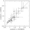 |
Fig. 1 Comparison of the photometric-z measured with 2SPD with those obtained by the COSMOS collaboration (Ilbert et al. 2009; Salvato et al. 2009). The dashed line is the bisector of the plane. |
Since the sample includes spectroscopically-confirmed quasars and other potential quasars whose SEDs appear power-law dominated, we use the method to derive the photometric redshifts, as introduced by Richards et al. (2001a,b) for quasars. They construct an empirical color-redshift relation based on the median colors of quasars from the SDSS survey as a function of redshift. Photometric redshifts are then determined by minimizing the χ2 between all four observed colors and the median colors (obtained by combining the five SDSS magnitudes, u′, g′, r′, i′, and z′) as a function of redshift.
We apply this method to the sources, which show a quasar-like SED and are detected in at least 2 SDSS bands, which include objects 22 and 35 (object 10 is excluded for this reason). As a sanity check, we include the two spectroscopically-confirmed quasars, namely 29 and 37, in this analysis. We also decided to analyze again objects with similar spectral shapes found by B13, namely COSMOS-FR I 32, 37, and 226, because they are potentially quasars for their power-law spectral behavior and the spectroscopically-confirmed quasar, COSMOS-FR I 236.
Table 4 reports the SDSS colors for these eight objects and Fig. 2 shows their χ2 curves. The χ2 minima that are smaller than the unity are not considered statistically significant. For the three spectroscopic quasars (29, 37 and COSMOS-FR I 236), the χ2 minima is consistent with the spectroscopic redshifts. For object 35, the χ2 minimum indicates a redshift of 1.8, which is different from that we derive from the SED modeling (1.03). We then finally change the classification of this source to quasar because of its SED and optical appearance and use as redshift  . Conversely, for the objects 22 and 33 and COSMOS-FR I 32, 37, and 226, the SDSS color fitting does not produce a reliable evidence for a redshift within the range of our interest. Therefore, we finally exclude these six objects (including object 10 that is not detected in SDSS bands) from the entire sample, since their photometric derivation is not convincing.
Summarizing, the sample selected in this work is reduced to 43 objects after the SED quality test, and we also exclude three sources from the sample studied by B13. Figure 3 summarizes our selection procedure, providing the number of the sources selected in each step of the selection.
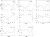 |
Fig. 2 Distribution of the χ2 function (see text) at varying redshift for objects 22, 29, 35, and 37 and for COSMOS-FR I 32, 37, 226, and 236 as obtained from the color-redshift relation using SDSS colors (Richards et al. 2001b). |
6.2. Host galaxy properties
We now focus on the properties of the host galaxies inferred from the SED modeling and in particular on their stellar populations for the 43 sources selected in this work, similarly to what done by B13.
The stellar mass of the galaxy, M∗, is one of the most robust results of the modeling. However, as discussed in B13, the presence of additional dust component to the OSP might affect the stellar mass estimate more than the inclusion of a YSP. The inferred mass range is ~1010 − 1011.5M⊙ (Fig. 4), as reported in Table 3.
Although the other host parameters derived from the SED modeling are less constrained than the estimate of the stellar content in the galaxy, we can globally state that the hosts are dominated by an OSP with an age of ~1−3 × 10⁹ years, which is similar to the results obtained by B13. Assuming that the emission at short wavelengths is associated with a YSP, the most significant UV component are reproduced by stellar populations of a few Myr (Table 3) with a contribution to the total mass of the galaxy less than 1%.
To qualitatively study the host type, the optical HST/ACS images provides the highest resolution view of the galaxy, although the maps are single orbit pointings. For the remaining (Subaru, CHFT, and Spitzer), optical and infrared images can provide a tentative indication of the host morphology for all the sources, apart from the four quasars, which show a point-like optical nucleus outshining the weaker galaxy. With a visual inspection of the multiband counterparts of the host, we can attempt to recognize the presence of clear spiral/disk galaxies or galaxies, which clearly differ from smooth ellipticals as observed at z ~ 1 (e.g., Huertas-Company et al. 2007). We do not see any evident late-type galaxy, but generally we can tentatively classify them as bulge-dominated objects. Only four sources (namely 18, 19, 38 and 41) show more irregular morphologies than classical undisturbed ellipticals (Fig. 5), which might be possible sign of an interaction with companion(s). The optical images of several objects show rich environments in their surroundings, similarly to what C09 found for the COSMOS-FR I sources.
6.3. Dust emission
Concerning the 43 objects selected in this work, dust emission is required to adequately model the SEDs of 16 objects (not considering the three quasars) due to the detection of emission at 24 μm, and significant excesses above the stellar emission are observed also at shorter infrared wavelengths in eight of these galaxies. However, as discussed in Sect. 5, the results of the SED fitting, that concern the dust components should not be used to infer dust properties. To explore the dust properties, we estimated the residuals between the best-fitting stellar model and the data-points, looking for an excess at the Spitzer wavelengths. We then integrated the residuals (by assuming that the spectrum is represented by a multiple step function) to obtain the infrared excess luminosity, LIR excess in the range covered by the Spitzer data, i.e. ~3−26 μm (see B13 for the details). The estimated dust properties are reported in Table 3.
The analysis misses the information on the dust content for the quasars, because they have been treated differently from the rest of the sample. We do not model their SEDs with stellar templates. Therefore, for the three quasars selected in this work, we estimate the dust luminosities with the method mentioned above and by assuming that the emission at the Spitzer wavelengths has only a dust origin. We also estimate the dust component for the quasar selected by C09 (COSMOS-FR I 236) with the same method. Table 5 shows the inferred IR luminosities for the quasars.
The dust luminosities of the sample selected in this work, as expressed as infrared excess luminosities, are in the range LIR excess ~ 1043−1045.5 erg s-1, similar to that found for the low-power radio galaxies studied by B13. The FR IIs cover the entire range of IR excess luminosities, showing also nondetections at 24 μm.
Similarly to what is done by B13, we also measured the spectral index of the infrared residuals over the OSP between 8 μm and 24 μm, αIR. Considering only significant (>3σ) excesses at 8 μm, this value can be estimated in eight cases with values spanning between αIR ~ 1 and −1. For the other eight objects with a 24 μm detection, the upper limit to the 8 μm flux translates into a lower limit of αIR ≳ − 1. For the four quasars (29, 35, 37, and COSMOS-FR I 236), we derive the spectral index again assuming that the emission at 8 μm has only a dust origin (Tables 3 and 5).
Since the temperatures associated with the thermal component are poorly constrained, we prefer to crudely estimate the overall dust temperature from the spectral index αIR. By assuming a single black-body dust component, the values of αIR translate into a temperature range of 750−1200 K and 350−600 K for αIR = −1 and 1, respectively. The derived temperature depends on redshift with the lower (upper) values of T being derived for z = 0.8 (z = 3).
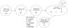 |
Fig. 3 Flow-chart describing our selection procedure. The number of sources that survive each step is reported inside each circle. See text for more details. |
6.4. UV excess
Inspection of the SED fits that are obtained with 2SPD indicates that the UV excesses (above the contribution of the OSP) are usually poorly constrained. Furthermore, the very stellar origin is not granted, and the UV excess might be due to an AGN contribution. It is necessary to introduce a model-independent criterion to assess which sources really show an UV excess, and to estimate its luminosity. We visually check all SEDs and search for sources with a substantial flattening in the SED at short wavelengths or with a change of the slope between the OSP and the emission in the UV band. A clear (marginal) UV excess in seen in 18 (12) sources, which is properly marked in Table 3. The remaining SEDs drop sharply in the UV and are well reproduced by the emission from the OSPs.
To quantify the UV contribution, for the objects showing an UV excess we measure the flux at 2000 Å in the rest frame, LUV, from the best fitting model, similarly to what done by B13. For the UV-faint sources, we estimate an upper limit on the UV emission. For the four quasars, we measure the flux at 2000 Å by using a power-law fit on the photometric data-points in the UV. In addition, we measure the upper limits to the UV excess also for the UV-faint objects studied in B13. The new UV excess measurements, which are included in the observed range 1041.5 ≲ LUV ≲ 1045.5 erg s-1, are reported in Table 5.
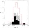 |
Fig. 4 Distribution of stellar masses (in M⊙) of our sample obtained with 2SPD. The solid line represents the sample of radio galaxies selected in this work: the filled histogram represents the FR II HPs, the cross-hatched histogram represents the remaining HPs, the back-slash shaded histogram represents the FR II LPs, and the empty histogram represents the remaining LPs. The red dashed histogram corresponds to the entire COSMOS RL AGN sample at high redshifts, which includes the sample selected by C09 and studied by B13. |
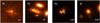 |
Fig. 5 HST/ACS images of the four sources, which show irregular optical morphologies. The image size is indicated in the panel. The white circle locates the position of the radio source. |
7. The RL AGN population at z ≳ 1 in the COSMOS field
The final sample of radio galaxies selected in the COSMOS field at z ≳ 1 counts 74 objects (precisely, 43 selected in this work plus 31 from B13). It includes four quasars, namely 29, 35, 37, and COSMOS-FR I 236. Figure 3 summarizes the selection procedure which drives to the final sample. The redshifts of the entire sample range between ~0.7 and ~3 with a median of 1.2. In the next sections, we study the properties of the entire population, gathering the results obtained in this work and those obtained by B13. Table 5 collects the information on the members of the sample.
The radio-loud AGN population in the COSMOS field at z ≳ 1.
7.1. Radio properties
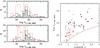 |
Fig. 6 Left panel: distribution of the rest-frame total radio luminosity (in erg s-1 Hz-1) at 1.4 GHz from the FIRST data (upper panel) and NVSS data (lower panel). The dashed lines correspond to the local FR I/FR II break used to separate the sample in HP and LP sources. The FR IIs distribution is represented by the back-slash shaded histogram. The dashed histogram represents the entire COSMOS RL AGN sample at high redshifts. Right panel: redshifts versus the rest-frame FIRST radio luminosity at 1.4 GHz (in erg s-1 Hz-1). The empty points are the LPs, and the full points are the HPs. The FR IIs are the triangles. The red squared points represent the sample studied by B13: LPs are the empty points and HPs the filled ones. The solid line represents the luminosity-redshift relation corresponding to the flux limit of the FIRST survey (between 1−0.6 mJy but we use 0.75 mJy for the plot.) |
Considering all the radio sources selected in the COSMOS field (see Table 5), most of them appear compact or marginally extended. Although it is possible that the nondetection of large-scale structures is a result of the high radio frequency at which the VLA-COSMOS catalog is carried out, it is likely that the compact sources are intrinsically small with sizes smaller than a few tens of kpc. The FR IIs, which show structures of, at most, some hundreds of kpc, are approximately one third of the entire sample, while the bona fide FR Is are two (both in C09 sample).
In Fig. 6 (left panel), we show the histograms of the rest-frame (using a radio spectral index α = 0.8) radio powers at 1.4 GHz measured with FIRST and NVSS, as reported in Table 58. The resulting luminosities are in the range 1031.5 − 1034.3 erg s-1 Hz-1, which straddle the local FR I/FR II break (L1.4 GHz ~ 1032.6 erg s-1 Hz-1 converting from 178 MHz to 1.4 GHz, Fanaroff & Riley 1974). For the entire population of high-z RL AGN in the COSMOS field, the median FIRST luminosity is 1032.59 erg s-1 Hz-1.
The radio luminosities of our sample are far larger than ~1030 erg s-1 Hz-1, which is the radio luminosity below which starburst activity may significantly contribute (e.g., Mauch & Sadler 2007; Wilman et al. 2008). Therefore, we can be confident that our sources are associated with RL AGN, where radio emission has a nonthermal synchrotron origin from the relativistic jets. Furthermore, the radio-loudness parameter (here measured as the radio-to-UV flux ratio, White et al. 2007) is always far higher than the threshold that separates radio-quiet from RL AGN.
Similarly to the approach used by B13, we prefer to separate the sample in high and low power (HP and LP, respectively) using the local FR I/FR II break as divide (see Table 5). This helps us investigate the properties of the sample and the role of the AGN, whose radio luminosity is a good estimator of its power. 40 out of 74 objects are HPs. All FR IIs are HPs with only three exceptions (namely 5, 13, and 15), although they are still with radio luminosities larger than 1032 erg s-1 Hz-1. With respect to B13, the inclusion of sources of higher fluxes corresponds to a broader range of luminosity at each given redshift (Fig. 6, right panel), thus improving our ability to explore the properties of high-z radio galaxies. Furthermore, it is noteworthy the redshift coverage of the FR II as broad as the entire observed range.
7.2. Global photometric properties of the sample
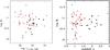 |
Fig. 7 Stellar masses (in M⊙) measured with 2SPD in relation with the rest-frame FIRST radio powers (in erg s-1 Hz-1) (left panel) and redshifts (right panel) of the sample. Black empty points are LPs, while filled black points are HPs. The FR IIs are the black triangles. The red squared points represent the sample studied by B13: LPs are the empty points and HPs the filled ones. |
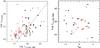 |
Fig. 8 Infrared excess luminosity (erg s-1) versus (left panel) rest-frame FIRST radio luminosity (erg s-1) and (right panel) spectral index from 8 to 24 μm estimated from the IR excess in the SED above the stellar emission (right panel). Black empty points are LPs, while filled black points are HPs. The FR IIs are the black triangles. The red squared points represent the sample studied by B13: LPs are the empty points and HPs the filled ones. The radio-IR correlation is the dashed line, and its parameters are shown in Table 6. |
The radio galaxies at z ≳ 1 selected in the COSMOS field are associated with hosts, which are in first approximation early-type galaxies. However, a further study is necessary to quantitatively investigate the morphology of the hosts to classify them more precisely. This will be addressed in a forthcoming paper.
Another important result is that the galaxies, which harbor our sample of distant RL AGN are massive and old. The median stellar mass of the hosts of these RL AGN is 5.8 × 10¹⁰M⊙. Figure 7 does not show any significantly evident relation between the stellar content and the radio power and the redshifts. If we divide the sample in LPs and HPs or FR IIs and no-FR IIs, no clear differences in stellar masses are present. Furthermore, the typical age of the dominant stellar population in those galaxies is a few Gyr-yr old.
The dust luminosities of the sample cover the range between 1043 to 1046 erg s-1 with a median value of 7 × 1043 erg s-1 (Fig. 8, left panel). Considering the radio classes, the LP and HP difference in dust luminosity is a factor ~3.3. The FR IIs cover the entire range of IR excess luminosities, also showing nondetections at 24 μm.
Figure 8 (right panel) shows a broad overlapping between the radio classes in dust luminosities and in IR spectral indices. This indicates that an increase of the AGN power (Lradio) is not necessarily associated with an increase of the dust luminosity and/or temperature. This denotes different possible contribution for the IR emission, star-formation, and/or AGN. However, we focus on the association between the dust and the AGN in Sect. 7.3.
The UV luminosities of the radio population range between LUV ~ 1041.5 and 1045.5 erg s-1 (Fig. 9) with a median value of 6 × 1042 erg s-1. Most LPs are faint in UV, while HPs show UV luminosities larger than LPs by a factor ~6. The HPs include most of the significant UV detections. The FR II sources cover the entire range of UV luminosities, showing also upper limits.
The global picture emerging from the high-z RL AGN population is substantially a mild bimodality. The LP are typically UV- and IR-faint, while the HPs are on the opposite side of the luminosity range. This behavior is not clearly a one-to-one relation and needs to be statistically tested (see next section).
We prefer to address the comparisons of our results with other samples of distant and local radio galaxies in a forthcoming paper.
Statistics.
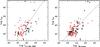 |
Fig. 9 UV luminosity (erg s-1) measured at 2000 Å versus (left panel) rest-frame FIRST radio luminosity (erg s-1) and (right panel) infrared excess luminosity (erg s-1). Black empty points are LPs, while filled black points are HPs. The FR IIs are the black triangles. The red squared points represent the sample studied by B13: LPs are the empty points and HPs are the filled ones. The dashed lines represent the linear correlations, whose parameters are reported in Table 6. |
7.3. The connection between radio, dust, and UV emission
In this section, we focus on the possible link between the nuclear and host properties for the entire sample of high-z RL AGN in the COSMOS field. The key point is to understand the origin of the IR and UV emission, which might be stellar or associated with the AGN. The radio luminosity is a fundamental indicator of the output energetics for a RL AGN. The IR and UV luminosities can provide clues on the amount of dust, star formation, and AGN contribution.
Figures 8 (left panel) and 9 compare the radio, IR, and UV luminosities, showing broad relations between them, although the dataset includes a large number of upper limits. A statistical approach, which considers the censored data is necessary to analyze the significance of such trends. We performed a statistical analysis using the Astronomy Survival Analysis (ASURV) package (Lavalley et al. 1992). We used the schmittbin task (Schmitt 1985) to calculate the associated linear regression coefficients for two sets of variables. Operatively, we carried out this procedure twice, obtaining two linear regressions: first, we consider the former quantity as the independent variable and the latter as the dependent one and second switching the roles of the variables. The best fit is represented by the bisector of these two regression lines. This followed the suggestion of Isobe et al. (1990) that considers such a method preferable for problems that require a symmetrical treatment of the two variables. To estimate the quality of the linear regression, we used the generalized Spearman’s rank order correlation coefficient, using the spearman task (Akritas 1989). Furthermore, since the sample covers a large range of redshifts, we tested the effects of such a quantity in driving these correlations (both luminosities depend on z2) estimating the Spearman Partial Rank correlation coefficient9. All the statistical parameters obtained are reported in Table 6.
Firstly, let us consider the relation between IR excess luminosity and 1.4-GHz FIRST power (Fig. 8, left panel). Using the generalized Spearman’s ρ test, the probability that a fortuitous correlation is P = 0.0007. However, considering the common dependence of the two luminosities on redshift, such a probability increases to P = 0.193.
Secondly, we focus on the UV excess and its possible link with radio power and dust luminosity (Fig. 9, left and right panels). For the radio-UV relation, the generalized rank coefficient ρ returns a probability of no correlation of P = 0.0001. The exclusion of the common redshift dependence with the partial rank coefficient yields a probability, P = 0.019 that a fortuitous correlation appears. Instead, for the UV-IR relation, according to the generalized Spearman’s rank coefficient, the probability that there is no correlation between the variables is P< 0.0001. The effect of the redshift, which might stretch the relation is negligible, as the value of the partial ρ slightly changes and the associated probability is still very small (P = 0.0007).
Since the four quasars present in the sample are among the brightest sources in the UV and IR bands, they potentially might drive the relations we find. We then remeasure the censored statistics parameters by excluding them. We obtain that the relations improve, apart from the radio-IR trend that slightly worsens. This indicates that the quasars are not responsible to drive the relations in the radio-IR-UV planes.
In summary, these tests enable us to conclude that the UV emission is significantly correlated with both the IR and the radio luminosities, the former being the stronger link. Conversely, the radio-IR relation might be real, but it has a non-negligible probability of being just driven by the common redshift dependence.
8. Summary and conclusions
We select a sample of radio sources in the COSMOS field by looking for objects at high redshifts (z ≳ 1) and extending a previous analysis focused on low-luminosity radio galaxies that is selected by C09 and studied by B13. While C09 selected the sample with the aim of searching for FR I candidates, we relaxed the C09 selection criteria to include all radio sources likely to be associated with galaxies at z ≳ 1, which is independent of the radio morphology. In particular, we include also objects with a FR II radio morphology in this analysis, and we do not set a high limit to the radio flux to obtain a complete view of the RL AGN phenomenon in this cosmological era. We then consider all radio sources with a flux > 1 mJy by looking for faint optical counterparts (I> 21), which is typical of radio galaxies in the redshift region of interest. We take advantage of the COSMOS multiband survey to select and identify their host galaxies with a careful visual inspection of the multiwavelength counterparts. The wide spectral coverage from the FUV to the MIR enables us to derive their SEDs and model them with our own code, 2SPD, which includes two stellar population of different ages and dust component(s). We obtained a sample formed by 74 members, most of them indeed having z ≳ 1.
The sample displays a large variety of radio and photometric properties, such as compact radio sources, FR Is, FR IIs, and quasars. We analyzed the properties of the SEDs of the sample analogously to what done by B13. Here, we summarize the main properties of the entire high-z COSMOS RL AGN population and briefly discuss them.
-
The photometric redshifts of the sample range between ~0.7 and 3 with a median of z = 1.2. Most of the sources have already a photo-z derivation from the COSMOS collaboration. However some do not mainly because their I-band magnitudes are beyond the I = 25 limit of the COSMOS photometric redshift catalog. Our photo-z measurements agree with those present in literature but are more robust because of the careful visual inspections of the multiband counterparts. For those source not present in the COSMOS catalog, we provide new photo-z estimates.
-
Once we obtain the photo-z, we infer their radio luminosities starting from their FIRST and NVSS radio fluxes. The rest-frame 1.4 GHz radio power distribution of the sample covers the range from 1031.5 to 1034.3 erg s-1 Hz-1, straddling the local FR I/FR II break (L1.4 GHz = 1032.6 erg s-1 Hz-1). Based on such a separation, we divide the sample in low- and high-power (LP and HP) sources. The radio sources are mostly compact (or slightly resolved) with sizes smaller than a few tens of kpc. Nevertheless, 21 objects show FR II radio morphology and are mostly HPs. Three quasars show compact radio structure, while one is associated with the center of a FR II.
-
The most robust result of the SED modeling is the derivation of the host stellar mass. The stellar content distribution covers values from ~1010 to 1011.5M⊙ with a median value of 6 × 10¹⁰M⊙. The LP and HP sources have similar stellar mass distributions.
-
Most sources show that SED is dominated by an old stellar population with an age of ~1−3 Gyr. However, significant excesses above the old stellar population are often observed in the IR and/or UV part of the SEDs.
-
A dust component is necessary to account for the 24 μm emission in 32 objects in the sample, and significant infrared excesses at even shorter wavelengths are observed in 13 of these galaxies (not considering the four quasars). The dust luminosities derived from these infrared excesses range from ~1043 to 1045.5 erg s-1. The dust temperatures estimated for these 13 objects are 350−1200 K; these values are dependent on the MIR spectral shape and redshifts.
-
The UV excess are present significantly in 30 sources and marginally in 19 sources. Estimates of the UV luminosities measured at 2000 Å (at rest frame) yield values in the range of 1041.5 − 1045.5 erg s-1.
-
We test the statistical significance of the radio-IR-UV luminosity relations, by considering censored statistics and the influence of the common dependence of luminosities on redshift. The UV emission is significantly correlated with both the IR and the radio luminosities, the former being the stronger link. Conversely, more doubts are present for the radio-IR relation.
A potential worry concerns the completeness at low fluxes. Indeed, a radio source with a total flux exceeding the adopted flux threshold of 1 mJy might be split into two separate components both below the flux limit. Such objects would not be included, causing incompleteness for radio fluxes between 1 and 2 mJy. We looked for sources in the COSMOS field between 0.6 (the FIRST catalog flux limit) and 1 mJy and then focused on the 20 objects detected by the COSMOS-VLA images. Thirteen of them have clear optical/IR counterparts and thus are unlikely to be one component of a double radio source. None of remaining seven shows evident FIRST double morphology on a scale of 180 arcsec. This suggests that the incompleteness caused by this effect is negligible.
A further problem appears to exist at higher radio fluxes. Twenty FIRST radio sources, including extended radio sources, are not part of the final sample: ten of them were discarded because they are not detected in the VLA-COSMOS survey, while in another 10 cases the association with an optical/IR counterpart is not possible or univocal. On the other hand, the identification of further ten FR II appears to be much more convincing. We do not expect more than a few false positives among them. With this approach, we favor the sample purity over its completeness. Another 6 objects were instead excluded, despite a successful counterpart identification, because the obtained modeling of their SEDs is less convincing than the others. While no more than a few percent of interlopers might be present (and all at high radio fluxes), we then conclude that a fraction as high as ~25% of incompleteness may affect the sample.
The total radio power distribution of the sample is rather broad and straddles the luminosity separation between FR Is and FR IIs in the local Universe. Note that the selected sample is, as planned, of much lower luminosity than classical samples of radio sources at similar redshifts and is comparable to those of the local population of radio galaxies. However, the radio luminosities of our sample are far larger than the level at which starburst activity may significantly contribute, and this indicates that they are genuine RL AGN. Unfortunately, we cannot establish the radio morphological classification for most of the sources; furthermore, the separation between the two FR types is less sharp at higher radio frequencies, considering that the rest-frame of these observations is ~3 GHz (at z = 1.2). Nonetheless, for the objects for which this is possible, the radio power generally predicts correctly their FR classification. In particular, all FR IIs are HPs with only three exceptions that still have radio luminosities larger than 1032 erg s-1 Hz-1. Local FR II radio galaxies exist at this lower radio power (e.g. Zirbel & Baum 1995; Best et al. 2005b).
The hosts of these high-z low-luminosity radio sources are massive (likely, early-type) galaxies, M∗ ~ 1010 to 1011.5M⊙. These values are similar with those derived for ellipticals in the COSMOS field in a similar range of redshifts (Ilbert et al. 2010). However, they display a wide range of properties. On the one hand, roughly half of the sample appears to be similar to those of local FR Is, which live in red massive early-type galaxies (e.g. Zirbel 1996; Best et al. 2005a; Smolčić 2009; Baldi & Capetti 2010) and show weaker nuclei (e.g. Chiaberge et al. 1999; Balmaverde et al. 2008; Baldi et al. 2010) than the galaxy emission. Indeed, among the least radio luminous objects, 28 sources are faint in both the UV and MIR bands. On the other hand, significant excesses in the UV and/or in the MIR band are often present. These excesses are observed in LP and HP sources, in contrast to low-z FR Is, which are typically UV faint and poor in dust (e.g. Chiaberge et al. 2002; Baldi & Capetti 2008; Hardcastle et al. 2009). These photometric properties are, instead, more familiar to local FR IIs, which typically show a bluer color (e.g. Baldi & Capetti 2008; Smolčić 2009) and a larger amount of dust (e.g. de Koff et al. 2000; Dicken et al. 2010) than the FR Is. These two behaviors correspond approximatively to the two radio classes, LPs and HPs. Overall, LPs (HPs) seem to better conform with the local FR Is (FR IIs) than HPs (LPs).
A key issue is to establish the origin of the MIR and UV emission, i.e. whether they are produced by the AGN and/or by star formation within the host. The statistical analysis indicates a connection between these two processes. However, this does not directly imply that for each source the IR and UV emission have the same origin. If we focus on the 13 sources, which show the significant MIR excess (to which we add the four quasars), the dust temperatures crudely derived from the spectral indices indicate values that largely exceed those measured in star forming galaxies (where Tdust ≲ 200 K, e.g., Dunne & Eales 2001; Hwang et al. 2010). This warrants that in these objects we deal with a dust heating mechanism from the AGN, where Tdust ≳ 300 K (e.g. Ogle et al. 2006). The UV properties of these sources are complex: two of them are undetected, while the remaining galaxies show a large scatter in the MIR/UV ratio. Furthermore, for our sample of radio galaxies, this ratio is LIR excess/LUV ~ 1−100, which is much higher than typical for quasars (Elvis et al. 1994). This suggests that nuclear obscuration also plays an important role, an indication also supported by their resolved optical appearance. The observed UV emission might still be nuclear in origin (e.g. due to scattering), but we cannot exclude a contribution (even dominant) from star formation.
For the remaining 57 objects, the situation is even more complex with the only common feature of an absence of an excess in the IRAC bands. Some of them show a 24 μm detection but are not always accompanied with an UV excess, and viceversa. The upper limits on the dust temperature for the galaxies detected in Spitzer are not sufficiently stringent to exclude an AGN origin. However, for the 28 objects which are faint in UV and IR band, the emission in such bands is likely ascribed to the galaxy and/or synchrotron radiation from the jet, as seen in local FR Is (e.g., Chiaberge et al. 2002; Baldi & Capetti 2008; Baldi et al. 2010).
The correlation between radio and UV indicates that a more powerful AGN has a larger probability to be associated with bluer host, but it remains unclear whether this is due to a larger star formation rate in the host or to a brighter AGN. The connection between radio and IR correlation has a significantly larger dispersion. A similar scatter is also found in the local RL AGN population (Dicken et al. 2009); here, this is clearly related to the different properties of the various classes of RL AGN.
In summary, the sample of the high-z RL AGN population in the COSMOS field includes active galaxies in which the contribution from AGN and stellar emission may be largely different from one object to the other. Weak AGN, which is dominated by an old stellar population, bright quasar-like AGN, and star formation, are the fundamental ingredients for the “recipe” to account for the range of properties of the sample, as broad as their radio morphology variety.
A further study is clearly necessary to investigate the properties of this sample, which also includes information on the X-ray and radio core data, already available from the COSMOS survey. Furthermore, a more detailed and quantitative comparison of this sample of RL AGN at high redshifts with samples of local and distant radio galaxies and with a population of quiescent galaxies at high z is required to explore their differences and similarities to shed further light on the galaxy-BH evolution across the cosmic time.
Online material
Appendix A: Radio maps, host identifications and SEDs
In this Appendix we include Tables A.1 and A.2, which present the final magnitudes and fluxes of the multiband counterparts of the radio sources of the sample. Figures A.1−A.3 show the VLA-COSMOS radio maps and the optical/IR images of the sources, for which we easily can identify the host, for the FR IIs that lack of a clear point-like emission from the radio core and for the sources that we fail in the host identification, respectively. Figure A.4 collects the modeled SEDs of the radio galaxies selected in this work.
COSMOS multiwavelength counterparts of the sample.
COSMOS GALEX and Spitzer counterparts of the sample.
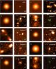 |
Fig. A.1 Images of the radio sources selected in the COSMOS field associated with a host galaxy with I> 21 (see Table 1). The left image for each source is from the VLA-COSMOS survey; the right image shows radio contours and the host identification in the band labelled on top. The image size in arcsec is marked on the bottom of each panel. When necessary, we mark the identified host galaxy with a white circle. |
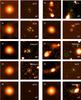 |
Fig. A.1 continued. |
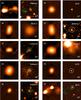 |
Fig. A.1 continued. |
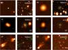 |
Fig. A.1 continued. |
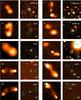 |
Fig. A.2 Host identification for FR IIs that lack of a clear point-like emission from the radio core. The labels and marks are as in Fig. A.1. |
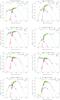 |
Fig. A.4 SEDs of the objects of the sample. The model is the green line, which includes the YSP (blue), the OSP (red), and the dust component(s) (cyan). The wavelengths on top of the plots correspond to observed wavelengths, while those on bottom are at rest frame. For the two spectroscopically confirmed quasars (objects 29 and 37) we only show the photometric points. |
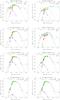 |
Fig. A.4 continued. |
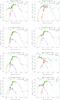 |
Fig. A.4 continued. |
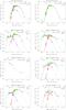 |
Fig. A.4 continued. |
 |
Fig. A.4 continued. |
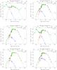 |
Fig. A.4 continued. |
FR I galaxies typically have a radio power lower than that of FR II sources with the FR I/FR II break set at L178MHz ~ 2 × 1033 erg s-1 Hz-1 (Fanaroff & Riley 1974). The transition is rather smooth and both radio morphologies are present in the population of sources around the break.
The COSMOS catalog is derived from a combination of the CFHT i∗ and Subaru i+ images to which the authors refer as I-band images
We consider a radius of 5100 arcsec because it corresponds to the radius of a circle, which circumscribes the “squared” COSMOS field. This allows us to include all the radio sources, which satisfy our selection criteria, but are located at the edges of the COSMOS field.
This number corresponds to each FIRST radio detection. Therefore, it does not correspond to the total number of radio sources, since double or even triple FIRST radio sources are present.
To identify the sources, we use a number ranging from 1 to 56 for simplicity. This number does not correspond to the nomenclature used by C09. The sources selected by C09 are named as “COSMOS-FR I”.
For the objects 12 and 13, we cannot measure their NVSS luminosities because their NVSS emissions are incorporated in the same source.
The Spearman Partial Rank correlation coefficient estimates the linear correlation coefficient between two variables by taking the presence of a third into account. If X and Y are both related to the variable z, the Spearman partial correlation coefficient is ![Mathematical equation: \hbox{$\rho_{XY,z}=\frac{\rho_{XY}\,-\,\rho_{Xz}\rho_{Yz}}{[(1\,-\,\rho_{Xz}^2)(1\,-\,\rho_{Yz}^2)]^{1/2}}$}](/articles/aa/full_html/2014/07/aa23906-14/aa23906-14-eq321.png)
Since the CFHT telescope is more sensitive and has a higher resolution than the images from the NOAO telescopes, this usually results in far smaller errors for the K -band magnitudes. In such cases, we prefer to use only the CFHT K -band data.
Acknowledgments
R.D.B. acknowledges the financial support from SISSA (Trieste) and from the Technion Institute (Haifa). We are grateful to the anonymous referee for the extremely useful comments to improve the paper and Sara Calabrese for the helpful support. This work is primarily based on the COSMOS data.
References
- Akritas, M. 1989, Aligned Rank Tests for Regression With Censored Data (Penn State Dept. of Statistics Technical Report) [Google Scholar]
- Baldi, R. D., & Capetti, A. 2008, A&A, 489, 989 [NASA ADS] [CrossRef] [EDP Sciences] [Google Scholar]
- Baldi, R. D., & Capetti, A. 2010, A&A, 519, A48 [NASA ADS] [CrossRef] [EDP Sciences] [Google Scholar]
- Baldi, R. D., Chiaberge, M., Capetti, A., et al. 2010, ApJ, 725, 2426 [NASA ADS] [CrossRef] [Google Scholar]
- Baldi, R. D., Chiaberge, M., Capetti, A., et al. 2013, ApJ, 762, 30 [NASA ADS] [CrossRef] [Google Scholar]
- Balmaverde, B., Baldi, R. D., & Capetti, A. 2008, A&A, 486, 119 [NASA ADS] [CrossRef] [EDP Sciences] [Google Scholar]
- Bardelli, S., Schinnerer, E., Smolčic, V., et al. 2010, A&A, 511, A1 [NASA ADS] [CrossRef] [EDP Sciences] [Google Scholar]
- Becker, R. H., White, R. L., & Helfand, D. J. 1995, ApJ, 450, 559 [NASA ADS] [CrossRef] [Google Scholar]
- Bertin, E., & Arnouts, S. 1996, A&AS, 117, 393 [NASA ADS] [CrossRef] [EDP Sciences] [Google Scholar]
- Best, P. N., Kauffmann, G., Heckman, T. M., et al. 2005a, MNRAS, 362, 25 [NASA ADS] [CrossRef] [Google Scholar]
- Best, P. N., Kauffmann, G., Heckman, T. M., & Ivezić, Ž. 2005b, MNRAS, 362, 9 [NASA ADS] [CrossRef] [Google Scholar]
- Bolzonella, M., Miralles, J., & Pelló, R. 2000, A&A, 363, 476 [NASA ADS] [Google Scholar]
- Calzetti, D., Armus, L., Bohlin, R. C., et al. 2000, ApJ, 533, 682 [NASA ADS] [CrossRef] [Google Scholar]
- Capak, P., Aussel, H., Ajiki, M., et al. 2007, ApJS, 172, 99 [NASA ADS] [CrossRef] [Google Scholar]
- Capak, P., Aussel, H., Ajiki, M., et al. 2008, VizieR Online Data Catalog: II/284 [Google Scholar]
- Chabrier, G. 2003, PASP, 115, 763 [NASA ADS] [CrossRef] [Google Scholar]
- Chiaberge, M., Capetti, A., & Celotti, A. 1999, A&A, 349, 77 [NASA ADS] [Google Scholar]
- Chiaberge, M., Macchetto, F. D., Sparks, W. B., et al. 2002, ApJ, 571, 247 [NASA ADS] [CrossRef] [Google Scholar]
- Chiaberge, M., Tremblay, G., Capetti, A., et al. 2009, ApJ, 696, 1103 [NASA ADS] [CrossRef] [Google Scholar]
- Condon, J. J., Cotton, W. D., Greisen, E. W., et al. 1998, AJ, 115, 1693 [NASA ADS] [CrossRef] [Google Scholar]
- de Koff, S., Best, P., Baum, S. A., et al. 2000, ApJS, 129, 33 [NASA ADS] [CrossRef] [Google Scholar]
- Dicken, D., Tadhunter, C., Axon, D., et al. 2009, ApJ, 694, 268 [NASA ADS] [CrossRef] [Google Scholar]
- Dicken, D., Tadhunter, C., Axon, D., et al. 2010, ApJ, 722, 1333 [NASA ADS] [CrossRef] [Google Scholar]
- Dunne, L., & Eales, S. A. 2001, MNRAS, 327, 697 [NASA ADS] [CrossRef] [Google Scholar]
- Elvis, M., Wilkes, B. J., McDowell, J. C., et al. 1994, ApJS, 95, 1 [NASA ADS] [CrossRef] [Google Scholar]
- Fabian, A. C., Sanders, J. S., Taylor, G. B., et al. 2006, MNRAS, 366, 417 [Google Scholar]
- Fanaroff, B. L., & Riley, J. M. 1974, MNRAS, 167, 31P [Google Scholar]
- Hardcastle, M. J., Evans, D. A., & Croston, J. H. 2009, MNRAS, 396, 1929 [NASA ADS] [CrossRef] [Google Scholar]
- Hewett, P. C., & Wild, V. 2010, MNRAS, 405, 2302 [NASA ADS] [Google Scholar]
- Hopkins, P. F., Hernquist, L., Cox, T. J., et al. 2006, ApJS, 163, 1 [Google Scholar]
- Huertas-Company, M., Rouan, D., Soucail, G., et al. 2007, A&A, 468, 937 [NASA ADS] [CrossRef] [EDP Sciences] [Google Scholar]
- Hwang, H. S., Elbaz, D., Magdis, G., et al. 2010, MNRAS, 409, 75 [NASA ADS] [CrossRef] [Google Scholar]
- Ilbert, O., Capak, P., Salvato, M., et al. 2009, ApJ, 690, 1236 [NASA ADS] [CrossRef] [Google Scholar]
- Ilbert, O., Salvato, M., Le Floc’h, E., et al. 2010, ApJ, 709, 644 [NASA ADS] [CrossRef] [Google Scholar]
- Isobe, T., Feigelson, E. D., Akritas, M. G., & Babu, G. J. 1990, ApJ, 364, 104 [NASA ADS] [CrossRef] [EDP Sciences] [Google Scholar]
- Jarosik, N., Bennett, C. L., Dunkley, J., et al. 2011, ApJS, 192, 14 [NASA ADS] [CrossRef] [Google Scholar]
- Koekemoer, A. M., Aussel, H., Calzetti, D., et al. 2007, ApJS, 172, 196 [NASA ADS] [CrossRef] [Google Scholar]
- Kroupa, P. 2001, MNRAS, 322, 231 [NASA ADS] [CrossRef] [Google Scholar]
- Lavalley, M., Isobe, T., & Feigelson, E. 1992, in Astronomical Data Analysis Software and Systems I, eds. D. M. Worrall, C. Biemesderfer, & J. Barnes, ASP Conf. Ser., 25, 245 [Google Scholar]
- Lilly, S. J., Le Fèvre, O., Renzini, A., et al. 2007, ApJS, 172, 70 [NASA ADS] [CrossRef] [Google Scholar]
- Maraston, C. 2005, MNRAS, 362, 799 [NASA ADS] [CrossRef] [Google Scholar]
- Mauch, T., & Sadler, E. M. 2007, MNRAS, 375, 931 [NASA ADS] [CrossRef] [Google Scholar]
- Ogle, P., Whysong, D., & Antonucci, R. 2006, ApJ, 647, 161 [NASA ADS] [CrossRef] [Google Scholar]
- Richards, G. T., Fan, X., Schneider, D. P., et al. 2001a, AJ, 121, 2308 [NASA ADS] [CrossRef] [Google Scholar]
- Richards, G. T., Weinstein, M. A., Schneider, D. P., et al. 2001b, AJ, 122, 1151 [NASA ADS] [CrossRef] [Google Scholar]
- Salpeter, E. E. 1955, ApJ, 121, 161 [Google Scholar]
- Salvato, M., Hasinger, G., Ilbert, O., et al. 2009, ApJ, 690, 1250 [CrossRef] [Google Scholar]
- Sanders, D. B., Salvato, M., Aussel, H., et al. 2007, ApJS, 172, 86 [Google Scholar]
- Schinnerer, E., Carilli, C. L., Scoville, N. Z., et al. 2004, AJ, 128, 1974 [NASA ADS] [CrossRef] [Google Scholar]
- Schinnerer, E., Smolčić, V., Carilli, C. L., et al. 2007, ApJS, 172, 46 [NASA ADS] [CrossRef] [Google Scholar]
- Schmitt, J. H. M. M. 1985, ApJ, 293, 178 [Google Scholar]
- Scoville, N., Aussel, H., Brusa, M., et al. 2007, ApJS, 172, 1 [NASA ADS] [CrossRef] [Google Scholar]
- Smolčić, V. 2009, ApJ, 699, L43 [NASA ADS] [CrossRef] [Google Scholar]
- Smolčić, V., Schinnerer, E., Scodeggio, M., et al. 2008, ApJS, 177, 14 [NASA ADS] [CrossRef] [Google Scholar]
- Spergel, D. N., Verde, L., Peiris, H. V., et al. 2003, ApJS, 148, 175 [NASA ADS] [CrossRef] [Google Scholar]
- Taniguchi, Y., Scoville, N., Murayama, T., et al. 2007, ApJS, 172, 9 [NASA ADS] [CrossRef] [Google Scholar]
- Trump, J. R., Impey, C. D., McCarthy, P. J., et al. 2007, ApJS, 172, 383 [NASA ADS] [CrossRef] [Google Scholar]
- White, R. L., Helfand, D. J., Becker, R. H., Glikman, E., & de Vries, W. 2007, ApJ, 654, 99 [NASA ADS] [CrossRef] [Google Scholar]
- Willott, C. J., Rawlings, S., Blundell, K. M., Lacy, M., & Eales, S. A. 2001, MNRAS, 322, 536 [NASA ADS] [CrossRef] [Google Scholar]
- Willott, C. J., Rawlings, S., Jarvis, M. J., & Blundell, K. M. 2003, MNRAS, 339, 173 [NASA ADS] [CrossRef] [Google Scholar]
- Wilman, R. J., Miller, L., Jarvis, M. J., et al. 2008, MNRAS, 388, 1335 [NASA ADS] [Google Scholar]
- York, D. G., Adelman, J., Anderson, Jr., J. E., et al. 2000, AJ, 120, 1579 [Google Scholar]
- Zirbel, E. L. 1996, ApJ, 473, 713 [NASA ADS] [CrossRef] [Google Scholar]
- Zirbel, E. L., & Baum, S. A. 1995, ApJ, 448, 521 [NASA ADS] [CrossRef] [Google Scholar]
All Tables
All Figures
|
Fig. 1 Comparison of the photometric-z measured with 2SPD with those obtained by the COSMOS collaboration (Ilbert et al. 2009; Salvato et al. 2009). The dashed line is the bisector of the plane. |
| In the text | |
|
Fig. 2 Distribution of the χ2 function (see text) at varying redshift for objects 22, 29, 35, and 37 and for COSMOS-FR I 32, 37, 226, and 236 as obtained from the color-redshift relation using SDSS colors (Richards et al. 2001b). |
| In the text | |
|
Fig. 3 Flow-chart describing our selection procedure. The number of sources that survive each step is reported inside each circle. See text for more details. |
| In the text | |
|
Fig. 4 Distribution of stellar masses (in M⊙) of our sample obtained with 2SPD. The solid line represents the sample of radio galaxies selected in this work: the filled histogram represents the FR II HPs, the cross-hatched histogram represents the remaining HPs, the back-slash shaded histogram represents the FR II LPs, and the empty histogram represents the remaining LPs. The red dashed histogram corresponds to the entire COSMOS RL AGN sample at high redshifts, which includes the sample selected by C09 and studied by B13. |
| In the text | |
|
Fig. 5 HST/ACS images of the four sources, which show irregular optical morphologies. The image size is indicated in the panel. The white circle locates the position of the radio source. |
| In the text | |
|
Fig. 6 Left panel: distribution of the rest-frame total radio luminosity (in erg s-1 Hz-1) at 1.4 GHz from the FIRST data (upper panel) and NVSS data (lower panel). The dashed lines correspond to the local FR I/FR II break used to separate the sample in HP and LP sources. The FR IIs distribution is represented by the back-slash shaded histogram. The dashed histogram represents the entire COSMOS RL AGN sample at high redshifts. Right panel: redshifts versus the rest-frame FIRST radio luminosity at 1.4 GHz (in erg s-1 Hz-1). The empty points are the LPs, and the full points are the HPs. The FR IIs are the triangles. The red squared points represent the sample studied by B13: LPs are the empty points and HPs the filled ones. The solid line represents the luminosity-redshift relation corresponding to the flux limit of the FIRST survey (between 1−0.6 mJy but we use 0.75 mJy for the plot.) |
| In the text | |
|
Fig. 7 Stellar masses (in M⊙) measured with 2SPD in relation with the rest-frame FIRST radio powers (in erg s-1 Hz-1) (left panel) and redshifts (right panel) of the sample. Black empty points are LPs, while filled black points are HPs. The FR IIs are the black triangles. The red squared points represent the sample studied by B13: LPs are the empty points and HPs the filled ones. |
| In the text | |
|
Fig. 8 Infrared excess luminosity (erg s-1) versus (left panel) rest-frame FIRST radio luminosity (erg s-1) and (right panel) spectral index from 8 to 24 μm estimated from the IR excess in the SED above the stellar emission (right panel). Black empty points are LPs, while filled black points are HPs. The FR IIs are the black triangles. The red squared points represent the sample studied by B13: LPs are the empty points and HPs the filled ones. The radio-IR correlation is the dashed line, and its parameters are shown in Table 6. |
| In the text | |
|
Fig. 9 UV luminosity (erg s-1) measured at 2000 Å versus (left panel) rest-frame FIRST radio luminosity (erg s-1) and (right panel) infrared excess luminosity (erg s-1). Black empty points are LPs, while filled black points are HPs. The FR IIs are the black triangles. The red squared points represent the sample studied by B13: LPs are the empty points and HPs are the filled ones. The dashed lines represent the linear correlations, whose parameters are reported in Table 6. |
| In the text | |
|
Fig. A.1 Images of the radio sources selected in the COSMOS field associated with a host galaxy with I> 21 (see Table 1). The left image for each source is from the VLA-COSMOS survey; the right image shows radio contours and the host identification in the band labelled on top. The image size in arcsec is marked on the bottom of each panel. When necessary, we mark the identified host galaxy with a white circle. |
| In the text | |
|
Fig. A.1 continued. |
| In the text | |
|
Fig. A.1 continued. |
| In the text | |
|
Fig. A.1 continued. |
| In the text | |
|
Fig. A.2 Host identification for FR IIs that lack of a clear point-like emission from the radio core. The labels and marks are as in Fig. A.1. |
| In the text | |
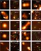 |
Fig. A.3 Images of the failed host identification. The labels and marks are as in Fig. A.1. |
| In the text | |
|
Fig. A.4 SEDs of the objects of the sample. The model is the green line, which includes the YSP (blue), the OSP (red), and the dust component(s) (cyan). The wavelengths on top of the plots correspond to observed wavelengths, while those on bottom are at rest frame. For the two spectroscopically confirmed quasars (objects 29 and 37) we only show the photometric points. |
| In the text | |
|
Fig. A.4 continued. |
| In the text | |
|
Fig. A.4 continued. |
| In the text | |
|
Fig. A.4 continued. |
| In the text | |
|
Fig. A.4 continued. |
| In the text | |
|
Fig. A.4 continued. |
| In the text | |
Current usage metrics show cumulative count of Article Views (full-text article views including HTML views, PDF and ePub downloads, according to the available data) and Abstracts Views on Vision4Press platform.
Data correspond to usage on the plateform after 2015. The current usage metrics is available 48-96 hours after online publication and is updated daily on week days.
Initial download of the metrics may take a while.