| Issue |
A&A
Volume 566, June 2014
|
|
|---|---|---|
| Article Number | A82 | |
| Number of page(s) | 17 | |
| Section | Numerical methods and codes | |
| DOI | https://doi.org/10.1051/0004-6361/201423408 | |
| Published online | 18 June 2014 | |
AME – Asteroseismology Made Easy
Estimating stellar properties by using scaled models⋆
Stellar Astrophysics Centre (SAC), Department of Physics and
AstronomyAarhus University,
Ny Munkegade 120,
8000
Aarhus C,
Denmark
e-mail:
This email address is being protected from spambots. You need JavaScript enabled to view it.
Received:
13
January
2014
Accepted:
5
April
2014
Abstract
Context. Stellar properties and, in particular stellar radii of exoplanet host stars, are essential for measuring the properties of exoplanets, therefore it is becoming increasingly important to be able to supply reliable stellar radii fast. Grid-modelling is an obvious choice for this, but that only offers a low degree of transparency to non-specialists.
Aims. Here we present a new, easy, fast, and transparent method of obtaining stellar properties for stars exhibiting solar-like oscillations. The method, called Asteroseismology Made Easy (AME), can determine stellar masses, mean densities, radii, and surface gravities, as well as estimate ages. We present AME as a visual and powerful tool that could be useful, in particular, in light of the large number of exoplanets being found.
Methods. AME consists of a set of figures from which the stellar parameters can be deduced. These figures are made from a grid of stellar evolutionary models that cover masses ranging from 0.7 M⊙ to 1.6 M⊙ in steps of 0.1 M⊙ and metallicities in the interval −0.3 dex ≤ [Fe/H] ≤ +0.3 dex in increments of 0.1 dex. The stellar evolutionary models are computed using the Modules for Experiments in Stellar Astrophysics (MESA) code with simple input physics.
Results. We have compared the results from AME with results for three groups of stars: stars with radii determined from interferometry (and measured parallaxes), stars with radii determined from measurements of their parallaxes (and calculated angular diameters), and stars with results based on modelling their individual oscillation frequencies. We find that a comparison of the radii from interferometry to those from AME yields a weighted mean of the fractional differences of just 2%. This is also the level of deviation that we find when we compare the parallax-based radii to the radii determined from AME.
Conclusions. The comparison between independently determined stellar parameters and those found using AME show that our method can provide reliable stellar masses, radii, and ages, with median uncertainties in the order of 4%, 2%, and 25%, respectively.
Key words: asteroseismology / stars: fundamental parameters / stars: low-mass / stars: solar-type
© ESO, 2014
1. Introduction
NASA’s Kepler mission (Koch et al.
2010) has provided photometric light curves of high precision, which has enabled
detecting solar-like oscillations in more than 500 stars (Chaplin et al. 2011). Asteroseismic scaling relations are generally used to
determine properties of such stars. (For a recent review on those issues see Chaplin & Miglio 2013). If one considers stars in
hydrostatic equilibrium, it follows from homology that since the dynamical time scale is
proportional to  (where
 is the mean density), the oscillation frequencies will be proportional to
 . In the
asymptotic approximation (see e.g. page 218 of Aerts et al.
2010), the frequency spectrum for a star can be written as a function of radial
order (n) and
angular degree (ℓ) as
. In the
asymptotic approximation (see e.g. page 218 of Aerts et al.
2010), the frequency spectrum for a star can be written as a function of radial
order (n) and
angular degree (ℓ) as  (1)Since
the frequencies scale with the square root of the mean density, the main regularity in the
asymptotic relation (Eq. (1)), which is the
large separation (Δν), will therefore be proportional to
(1)Since
the frequencies scale with the square root of the mean density, the main regularity in the
asymptotic relation (Eq. (1)), which is the
large separation (Δν), will therefore be proportional to
 .
The parameters D0 and ε will depend on the detailed
internal structure of a given star and can, for instance, be used to estimate its age.
.
The parameters D0 and ε will depend on the detailed
internal structure of a given star and can, for instance, be used to estimate its age.
The large separation can be found from the sound-speed integral: 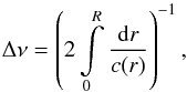 (2)where R is the stellar radius, and
c(r) the sound-speed in the stellar
interior. We use this fundamental asteroseismic parameter Δν to estimate the stellar
mean density. It has been common practice to also use the frequency at maximum oscillation
power (νmax) to measure the gravity of a given star
since observationally it has been shown to be proportional to the acoustic cut-off frequency
in the atmosphere (which scales with
(2)where R is the stellar radius, and
c(r) the sound-speed in the stellar
interior. We use this fundamental asteroseismic parameter Δν to estimate the stellar
mean density. It has been common practice to also use the frequency at maximum oscillation
power (νmax) to measure the gravity of a given star
since observationally it has been shown to be proportional to the acoustic cut-off frequency
in the atmosphere (which scales with  ).
While the observational link to the acoustic cut-off frequency is established (Stello et al. 2009a), we still need to better understand
the theoretical background for this relation (Belkacem et
al. 2011, 2013). A problem in relation to
the use of νmax is that there is a tight relation
between νmax and Δν (see Stello et al. 2009a). This is why we in the present study only consider
Δν and not
νmax.
).
While the observational link to the acoustic cut-off frequency is established (Stello et al. 2009a), we still need to better understand
the theoretical background for this relation (Belkacem et
al. 2011, 2013). A problem in relation to
the use of νmax is that there is a tight relation
between νmax and Δν (see Stello et al. 2009a). This is why we in the present study only consider
Δν and not
νmax.
Obtaining stellar parameters such as mass, radius, and age through detailed modelling
(modelling based on individual oscillation frequencies) for just one star that shows
solar-like pulsations can be a very time-consuming task. As an alternative, one or more of
the analysis pipelines described in, for instance, Quirion
et al. (2010) (SEEK), Mathur et al. (2010),
Stello et al. (2009b) (RADIUS), Basu et al. (2010), and Gai et al. (2011) can be utilised. However, this grid-based modelling does not
offer a very transparent procedure, and inconsistencies can occur between the mean density
derived using the large separation ( ) and
the one found using the grid-determined mass and radius
(
) and
the one found using the grid-determined mass and radius
( ).
This is primarily an effect of mass and radius being determined individually (Quirion et al. 2010) and the fact that grid-based
modelling sometimes yield bimodal parameter distributions.
).
This is primarily an effect of mass and radius being determined individually (Quirion et al. 2010) and the fact that grid-based
modelling sometimes yield bimodal parameter distributions.
White et al. (2011a) discuss the potential of constraining stellar masses and ages for main-sequence (MS) and sub-giant solar-like oscillators using diagrams based on their pulsation properties, such as the Christensen-Dalsgaard and the ε diagrams. However, ε can be hard to constrain (White et al. 2011b), and the Christensen-Dalsgaard diagram requires the value of the small separation (δν) to be known, but this is usually not available. The reason for this is that to find δν, some modes with ℓ = 2 need to be discernible in the power spectrum, which is often not the case.
Therefore we have developed a method of obtaining self-consistent mean densities, along with other stellar parameters, in an easy and fast way for MS and sub-giant stars that show solar-like oscillations. We consider this method to be transparent because it is easy to follow since, from considering the figures, it is straightforward to see what effect a small change in one of the input parameters would have on the result. By scaling to the Sun we have made our method less sensitive to the stellar models and evolution code used. We call this method AME – Asteroseismology Made Easy. The aim of this paper is to present AME as a powerful and visual tool that does not need the frequency of maximum power to yield basic stellar properties.
2. The AME models
AME allows for determining stellar mean density (),
mass (M), age
(τ), and by
inference surface gravity (g) and radius (R) of MS and sub-giant stars
showing solar-like oscillations. The method is based on a grid of models spanning a range in
metallicity and mass from which we have made plots that can be used to determine all those
parameters. We wanted to make our determination of the stellar parameters as insensitive as
possible to the choice of evolution code used. Therefore, we have scaled all results to the
Sun and tested the effects on the Hertzsprung-Russell (H-R) diagram of using different
evolution codes.
2.1. The importance of the evolution code
We tested the sensitivity of our method to the choice of stellar evolution code and solar chemical composition. We did this to make sure that the results that come out of AME are not affected to any significant degree by either of the two. To facilitate this test, we computed a series of evolution tracks and compared them qualitatively.
We calculated a series of four models using each of the three evolution codes MESA (Modules for Experiments in Stellar Astrophysics, Paxton et al. 2011, 2013), ASTEC (Aarhus STellar Evolution Code, Christensen-Dalsgaard 2008), and GARSTEC (Garching Stellar Evolution Code, Weiss & Schlattl 2008). These four models consist of two that use the solar abundances by Grevesse & Sauval (1998, hereafter GS98) and two that use the newer abundances by Asplund et al. (2009, hereafter A09). For each set of abundances we computed an evolution track for a 1.0 M⊙ and for a 1.2 M⊙ star.
The tracks were calculated using input physics that were as similar as possible for the three evolution codes. The input microphysics that we used were the 2005 update of the OPAL EOS (Rogers et al. 1996; Rogers & Nayfonov 2002), the OPAL opacities (Iglesias & Rogers 1996) supplemented by the Ferguson et al. (2005) opacities at low temperatures, the NACRE nuclear reaction rates (Angulo et al. 1999) with the updated 14N(p,γ)15O reaction rate by Formicola et al. (2004), and no diffusion or settling.
For the macrophysics, we neglected convective overshoot and used an Eddington T − τ relation as the atmospheric boundary condition. We treated convection using the mixing-length theory of convection, in the case of GARSTEC in the formulation of Kippenhahn et al. (2013), and in the cases of ASTEC and MESA in the formulation of Böhm-Vitense (1958).
Before the tracks were made, each of the codes was calibrated to the Sun using each of the GS98 and A09 abundances. This calibration was performed by adjusting the mixing-length parameter (αML) and the initial helium (Y0) and heavy-element (Z0) mass fractions until a model with the mass of the Sun had the solar radius and luminosity and a surface value of Z/X in accordance with the abundances chosen, at the age of the Sun. The target values of Z/X were (for the present-day photosphere) (Z/X)GS98 = 0.0231 and (Z/X)A09 = 0.0181 (Asplund et al. 2009). The twelve resulting tracks can be found in Fig. 1.
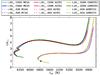 |
Fig. 1 H-R diagram comparing evolution tracks made with MESA, ASTEC, and GARSTEC for stars of mass 1.0 M⊙ and 1.2 M⊙ with two different chemical compositions: GS98 and A09. The star is the Sun. |
There are two places where the evolution tracks in Fig. 1 differ slightly. This is at the bottom of the red giant branch (RGB) and in the 1.2 M⊙ case around the MS turn-off. The difference at the bottom of the RGB is not really relevant here since the stars in this region are not the prime focus of AME. The difference around the MS turn-off is to be expected since the change from a radiative core on the MS to a convective core happens at a mass just around 1.2 M⊙, and as a consequence there is high sensitivity to any small differences between the codes at this particular mass. This is why this mass was included in the test in the first place, and the codes do not differ drastically. The GARSTEC tracks show clear signs of convective cores for both solar compositions (GS98 and A09), and the ASTEC and MESA tracks also show convective cores in both cases, but these are very small when using the A09 abundances. The difference in the size of the convective core when using the GS98 and A09 abundances can be understood since the GS98 composition has a higher abundance of the CNO-elements than the A09 composition. This higher CNO-element abundance will cause the CNO cycle to be more important, which will lead to a slightly higher temperature dependence in the core since the CNO cycle depends more strongly on the temperature than the pp-chain does. Thereby, the temperature gradient in the core will be slightly larger and therefore a star with the GS98 abundances will be more prone to having a convective core (see also Christensen-Dalsgaard & Houdek 2010).
Thus, the three codes give quite similar results. This is reassuring because it means that the decision to use MESA to make the stellar models for AME does not significantly affect the results. Also, we chose to use the A09 abundances to make the AME grid of models, and it is evident from Fig. 1 that this choice does not have a strong impact on the results either. However, it is not clear from Fig. 1 how the ages of the different tracks compare. We have found that for the most evolved star that AME has been used on, the ages coming from the different tracks agree at the 5% level. This means that also the ages from AME are fairly insensitive to the choice of evolution code and set of abundances, at least to the uncertainty level of the ages from AME (see Sect. 6.3).
2.2. Grid of scaled models
We used stellar models obtained with MESA to generate a grid of models with masses spanning 0.7 M⊙ − 1.6 M⊙ in steps of 0.1 M⊙ and metallicities in the range −0.3 dex ≤ [Fe/H] ≤ +0.3 dex in increments of 0.1 dex. We chose to keep the stellar models simple, which meant that we used MESA with the input physics described in Sect. 2.1 except that we used the MESA photospheric tables (Paxton et al. 2011) instead of an Eddington grey atmosphere. The value of the mixing length parameter was kept fixed at the value found by calibrating to the Sun: αML = 1.71.
The hydrogen- (X), helium- (Y), and heavy-element mass
fractions (Z)
obtained from the solar calibration assuming the A09 abundances were used to compute the
stellar mass fractions assuming ![Mathematical equation: \begin{equation} \label{eq:FeH} [\mathrm{Fe}/\mathrm{H}] = [\mathrm{M}/\mathrm{H}] = \log \left( \frac{Z} {X} \right) _* - \log \left( \frac{Z}{X} \right) _\sun , \end{equation}](/articles/aa/full_html/2014/06/aa23408-14/aa23408-14-eq51.png) (3)where the subscript
∗ indicates the
star, and the initial solar mixture is known from our solar calibration: X⊙ = 0.71247 and
Z⊙ =
0.01605. (We use the modelled solar composition when the Sun arrived on
the ZAMS in Eq. (3), since our models
contain no diffusion or settling). We used a helium evolution of
(3)where the subscript
∗ indicates the
star, and the initial solar mixture is known from our solar calibration: X⊙ = 0.71247 and
Z⊙ =
0.01605. (We use the modelled solar composition when the Sun arrived on
the ZAMS in Eq. (3), since our models
contain no diffusion or settling). We used a helium evolution of
 (Balser 2006) with a Big Bang nucleosynthesis helium mass fraction of
YBBN =
0.2488 (Steigman 2010) and
heavy-element mass fraction of ZBBN = 0. This, in combination with the
well-known relation X +
Y + Z = 1, allowed us to determine
the stellar mass fractions for a given metallicity.
(Balser 2006) with a Big Bang nucleosynthesis helium mass fraction of
YBBN =
0.2488 (Steigman 2010) and
heavy-element mass fraction of ZBBN = 0. This, in combination with the
well-known relation X +
Y + Z = 1, allowed us to determine
the stellar mass fractions for a given metallicity.
All of the models in the grid were evolved until they reached a large separation of 20 μHz since this does not happen until far beyond the MS that is the prime focus of AME.
Median mass and radius differences caused by changes in the input physics.
2.3. Implications of the chosen input physics
Since we chose to use simple input physics for our grid of models, we have made choices that may lead to significant systematic errors in our results (see for instance Bonaca et al. 2012, for a discussion of the mixing length parameter). These choices include neglecting diffusion and overshoot and only considering one value of the mixing length parameter and the helium evolution.
To investigate the likely size and direction of any such systematics, we tested the
influence of changed input physics on our results. We did this by computing evolutionary
tracks for five stellar masses (M =
1.0,1.1,1.2,1.3,1.4
M⊙) where we changed one of our
assumptions at a time (using just a single metallicity). We computed two sets of tracks
that used a different mixing length parameter (one higher than our solar calibration and
one lower: αML =
1.51 and αML = 1.91), one set of tracks that
included overshoot (with a value fov = 0.015), one set that incorporated
element diffusion, and two sets that used a different helium evolution (again, one with a
lower value and one with a higher value than the one we chose:
 and
and
 ). Subsequently, we
compared the masses and radii derived for 20 artificial stars using the tracks with our chosen input physics to
the results obtained when using each of the sets of tracks with an altered input physics.
The median difference (in the sense of changed physics – chosen
physics) can be seen in Table 1.
). Subsequently, we
compared the masses and radii derived for 20 artificial stars using the tracks with our chosen input physics to
the results obtained when using each of the sets of tracks with an altered input physics.
The median difference (in the sense of changed physics – chosen
physics) can be seen in Table 1.
As can be seen from the table, the systematic effects that may be caused by neglecting
convective overshoot or diffusion are rather weak for the selected mass range, while they
are significant when choosing only a single value for αML and
 .
Nevertheless, we chose to do this to keep the input physics and the method itself simple.
As a consequence, these systematic effects should be borne in mind (and note that we
solely quote internal uncertainties throughout this paper).
.
Nevertheless, we chose to do this to keep the input physics and the method itself simple.
As a consequence, these systematic effects should be borne in mind (and note that we
solely quote internal uncertainties throughout this paper).
Valle et al. (2014) has obtained similar values for the effect on mass and radius from changing the value of the mixing length parameter or the helium evolution. However, they consider a lower mass range (0.8 ≤ M/M⊙ ≤ 1.1). This may explain why they find diffusion to be more significant than we do since diffusion is known to play an important role in the Sun, but seem to be counteracted by processes like radiative levitation for F stars (Turcotte et al. 1998). This is also one of the reasons we chose to neglect diffusion. (Radiative levitation is not included in MESA, see Paxton et al. 2011).
The systematic uncertainties caused by neglecting convective overshoot is not considered by Valle et al. (2014), but we find that for the masses we have investigated, it does not significantly influence the mass or the radius. However, it can affect the age. Including overshoot will cause typical age differences that are vanishingly small compared to the age uncertainties in AME (see Sect. 6.3), but during the MS turn-off, the age differences can be in the order of 15%, which is quite significant (see for instance Silva Aguirre et al. 2011, who find a similar value). However, this phase of evolution is very fast, and the chance of catching a star during this evolutionary step is fairly low. Therefore we have assumed that convective overshoot can be disregarded.
It is worth noting that while the systematics are not negligible, they are still less than the median uncertainties on mass, radius, and age returned by AME, which are 4%, 2%, and 25%, respectively (see Sect. 6.3). Also, we have found that our results are in excellent agreement with the stellar parameters found in the literature (see Sects. 5 and 6).
3. The AME figures
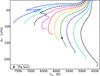 |
Fig. 2 Evolutionary tracks for models with varying mass and solar metallicity plotted in a variation of a classic H-R diagram (Δν plotted against Teff). The star shows the location of the Sun and the different line colours represent different masses starting with the black 0.7 M⊙ line on the far right going in increments of 0.1 M⊙ to the blue 1.6 M⊙ line on the far left. |
The foundation of AME is the grid of models created using MESA, which we described in Sect. 2.2. We used some of the output parameters from each model in the grid to create three types of plots. The idea of using plots to obtain stellar parameters came from the observation that evolutionary tracks in an H-R diagram look approximately similar for lines of neighbouring mass and metallicity. This is illustrated in Fig. 2, which shows Δν as a function of Teff for models of solar metallicity. Based on this, we expected to be able to more or less make lines of different masses and metallicities overlap if we adjusted the axes – both in a plot like Fig. 2 and when plotting other stellar properties against each other.
The model outputs that we used to make the AME plots are the large separation, the mass,
the age, the temperature, the metallicity, and the mean density. We scaled the found large
separation by the ratio of the observed solar large separation to the modelled solar large
separation (from the MESA solar calibration, calculated from the sound-speed integral in Eq.
(2)):
 , where the observed value
of the solar large separation is from Toutain &
Fröhlich (1992). This was done in order to correct for the difference between the
Δν found from
(2), which does not take near-surface
effects into account, and the observed Δν, found as Δν = νn
+1,0 −
νn,0, which is affected by
near-surface effects. We have checked that the ratio found for the Sun is consistent with
the ratios of Δν found from model frequencies to Δν found from the sound-speed
integral (Eq. (2)) for other stars to around
1% and that this is
independent of mass, chemical composition, and evolutionary state. A similar discrepancy has
been found by Chaplin et al. (2014) between the
Δν found from
the oscillation frequencies and the one calculated from the scaling relation
, where the observed value
of the solar large separation is from Toutain &
Fröhlich (1992). This was done in order to correct for the difference between the
Δν found from
(2), which does not take near-surface
effects into account, and the observed Δν, found as Δν = νn
+1,0 −
νn,0, which is affected by
near-surface effects. We have checked that the ratio found for the Sun is consistent with
the ratios of Δν found from model frequencies to Δν found from the sound-speed
integral (Eq. (2)) for other stars to around
1% and that this is
independent of mass, chemical composition, and evolutionary state. A similar discrepancy has
been found by Chaplin et al. (2014) between the
Δν found from
the oscillation frequencies and the one calculated from the scaling relation
 (see Sect. 1).
To take the small difference into account and not end up with an erroneously low error bar on the stellar parameters, we set a lower limit on the uncertainty on Δν of 1%. Thus if a star has a lower uncertainty on the large separation than 1%, we inflate this uncertainty to be 1% before we use AME. This means that the plots (created using models) can (and should) be used with observed values of the large separation. By always scaling to the Sun, it should also be possible to compensate for any systematic effect that is shared by all the models in the grid.
From the three types of plots, the mass, mean density, and age can be determined based on
only the large separation (Δν), the effective temperature (Teff), and the
metallicity ([Fe/H
]) of the star, using linear interpolation between the lines in the
plots. From the mean density and the mass, the radius and surface gravity can be derived
using Eqs. (4) and (5), respectively: ![Mathematical equation: \begin{eqnarray} \label{eq:sca_R} \frac{R}{R_\odot} &=& \left( \frac{M}{M_\odot} \right)^{1/3} \left(\frac{\bar{\rho}}{\bar{\rho}_\odot}\right) ^{-1/3} , \\[3mm] \label{eq:sc_g} \frac{g}{g_\odot} &=& \left( \frac{M}{M_\odot} \right)^{1/3} \left(\frac{\bar{\rho}}{\bar{\rho}_\odot}\right) ^{2/3} \cdot \end{eqnarray}](/articles/aa/full_html/2014/06/aa23408-14/aa23408-14-eq89.png) There
are several versions of each type of plot that each corresponds to a region of the
(Δν,Teff, [Fe/H]) parameter space with a small overlap. An
example of each type of plot can be seen in Figs. 3
(mass), 4 (mean density), and 5 (age) in Sect. 4. The full set of
figures consisting of three mass plots, six mean-density plots, and six age plots can be
found in the online material Appendix A.
There
are several versions of each type of plot that each corresponds to a region of the
(Δν,Teff, [Fe/H]) parameter space with a small overlap. An
example of each type of plot can be seen in Figs. 3
(mass), 4 (mean density), and 5 (age) in Sect. 4. The full set of
figures consisting of three mass plots, six mean-density plots, and six age plots can be
found in the online material Appendix A.
3.1. The figure axes
The axes on the plots have been chosen so that the different masses can be distinguished in the type of plot used to determine stellar mass and make the mass and metallicity have as little effect as possible when establishing the stellar mean density and age. Thus the axes are the results of iterations based on physical expectations and the attempt to make the lines collapse. Below, we describe the axes of each plot type.
3.1.1. The axes of the mass plots
For the type of plot used to determine the masses (an example can be seen in Fig. 3), we have used axes of the form Teff · 10a · [Fe/H] and Δν · 10−b · [Fe/H]. The large separation decreases monotonically through the evolution of a solar-like oscillator, whilst lines of constant density across evolution tracks in an H-R diagram have different temperatures. Therefore a temperature versus large separation plot should separate the different masses out. The small metallicity dependence given by the variables a and b is used to collapse the lines of differing metallicity, but identical mass. The coefficients vary from plot to plot, but in each case the values were chosen that were found empirically to best collapse the lines.
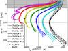 |
Fig. 3 Plot used to determine the mass of α Cen A. The colours give the masses of the lines ranging from 0.7 M⊙ (black) in the right of the figure in steps of 0.1 M⊙ to 1.3 M⊙ (magenta/purple) in the left of the figure. The different line types give the metallicity. The star shows the location of α Cen A in the figure. The shaded area in the top indicates the region where another mass plot would be more suitable. |
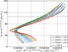 |
Fig. 4 Plot used to determine the mean density of α Cen A. The colours represent different masses: 0.7 M⊙ (black), 0.8 M⊙ (light blue), 0.9 M⊙ (blue), 1.0 M⊙ (green), 1.1 M⊙ (yellow), and 1.2 M⊙ (red), whilst the line styles give the metallicity of a given line. The location of α Cen A in the plot is marked by the horizontal, black, dashed line. |
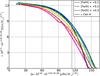 |
Fig. 5 Plot used to determine the age of α Cen A. The colours represent different masses: 0.7 M⊙ (black), 0.8 M⊙ (light blue), 0.9 M⊙ (blue), 1.0 M⊙ (green), 1.1 M⊙ (yellow) 1.2 M⊙ (red), and 1.3 M⊙ (magenta/purple), whilst the line types indicate the metallicity of a given line. The location of α Cen A in the plot is marked by the vertical, black, dashed line. |
3.1.2. The axes of the mean-density plots
In the type of plot used to infer the mean density, the main relation that we used is
the well-known asteroseismic scaling relation  (Kjeldsen & Bedding 1995; Bedding & Kjeldsen 2010), which was also
mentioned in Sect. 1. Following it,
(Kjeldsen & Bedding 1995; Bedding & Kjeldsen 2010), which was also
mentioned in Sect. 1. Following it,
 is expected to be reasonably constant for all stars. Therefore, this is used on the
x axis
since it results in high precision on the mean density. It is used in combination with a
small metallicity dependence as in the mass plots and a slight mass dependence. These
serve the purpose of collapsing the lines to the greatest extent possible.
is expected to be reasonably constant for all stars. Therefore, this is used on the
x axis
since it results in high precision on the mean density. It is used in combination with a
small metallicity dependence as in the mass plots and a slight mass dependence. These
serve the purpose of collapsing the lines to the greatest extent possible.
On the other axis, we have used a combination of the form Δν · Mc · 10−d · [Fe/H]. Except for the small metallicity dependence that serves the same purpose as previously, the axis is thus a product of the large separation and the mass. The exponent of the mass (c) varies a little from plot to plot (again, depending on what is found to best collapse the lines), but it is in the order of one. Based on the approximate proportionality on the MS of radius and mass, the product of the mass to a power in the vicinity of unity and the large separation will be roughly similar for all stars on the MS, which explains why this is on the y axis.
3.1.3. The axes of the age plots
The x axis of the age plots has the form Δν · Mf · 10g · [Fe/H], where g can be both negative and positive, but is around zero and f is positive and around one. This is therefore much the same axis as was used on the y axis of the mean-density plots.
The y axis features the age of the star and the mass to an approximate exponent of four in addition to a now well-known term in metallicity to help collapse the lines. The use of the product τ · M4 was based on the nuclear time scale that is given by tnuc ∝ ML-1 (Eq. (1.90) of Hansen et al. 2004) and the luminosity-mass relation for low-mass stars L ∝ M5.5 (p. 29 of Hansen et al. 2004). Combining these two and taking the nuclear time scale as an estimate of the total stellar age, it is found that the product of stellar age and mass to the power of ~4.5 is expected to be more or less similar for all stars. This is why we used it on the y axis of the age plots.
4. The 3 steps in using AME: α Cen A
Literature values for stars with results from detailed modelling.
AME has been used on a number of stars that either have radii determined from interferometry (and measured parallaxes), radii based on parallax measurements (and calculations of the stellar angular diameters), or parameters found from detailed modelling (in some cases in combination with other methods). One of these stars is the solar-like star α Cen A, whose values of its spectroscopic parameters, large separation, mass, radius, and age can be found in Table 2, along with the properties of the other stars with results from detailed modelling (listed in order of decreasing large separation). To illustrate the use of AME, we describe in Sects. 4.1, 4.2, and 4.3 below how we used AME to obtain the stellar parameters for α Cen A. Furthermore, in Sect. 4.4 we explain how we determined the internal uncertainties on the stellar parameters.
4.1. Step 1: Determining the stellar mass
The first step when using AME on α Cen A was to find the mass. Depending primarily on the known values of the effective temperature and large separation, the appropriate version of the mass plot had to be used, and we chose the relevant one for α Cen A. The plot can be seen in Fig. 3 with the location of α Cen A marked. This plot was chosen firstly because it encompassed the parameters of α Cen A, and secondly because the star did not fall in the grey-shaded region of the plot.
It can easily be seen from this figure that α Cen A lies almost on top of the 1.1 M⊙ lines. By considering the metallicity of the star, we found the mass to be M = 1.10 M⊙ using linear interpolation between the lines of different masses and metallicities. It should be noted that this value is in excellent agreement with the value listed in Table 2 found using the binarity of the α Cen system.
4.2. Step 2: Finding the mean stellar density
The second step was to find the mean density of α Cen A. This could be done by using the suitable mean-density plot after we had determined the mass. The mean-density plot that we used can be seen in Fig. 4. This particular plot was chosen because it covered the mass and metallicity of α Cen A.
From the expression on the y axis, we calculated the y-axis location of
α Cen A in
the plot, as marked in Fig. 4. The mean density of
α Cen A was
now determined by first interpolating the crossing of the dashed line (the y-axis location of
α Cen A)
with the lines of surrounding masses (1.1
M⊙ and 1.2 M⊙) and
metallicities (+0.2 dex and
+0.3 dex) to find the
position of the crossing between the horizontal dashed line and a line with the
metallicity and mass of α Cen A. This gave us the position on the
x axis of
α Cen A and
thereby the value of ![Mathematical equation: \hbox{$\bar{\rho}/\Delta \nu^2 \cdot M^{0.01} \cdot 10^{-0.015 \cdot [\mathrm{Fe}/\mathrm{H}]}$}](/articles/aa/full_html/2014/06/aa23408-14/aa23408-14-eq219.png) . Using the large separation and
the metallicity from Table 2 along with the mass
found from the previous plot, we then calculated the mean density of α Cen A to be
. Using the large separation and
the metallicity from Table 2 along with the mass
found from the previous plot, we then calculated the mean density of α Cen A to be
 .
.
From the mass and mean density, the radius and surface gravity of α Cen A were computed using Eqs. (4) and (5), respectively. We found the radius to be R = 1.22 R⊙ and a surface gravity of g = 0.738 g⊙. Using a solar surface gravity of, for instance, log g⊙ = 4.43789 dex [cgs]1, this value can be converted into classical units: log g = 4.31 dex [cgs]. It is noteworthy that the found radius agrees very well with the one from the literature (see Table 2).
4.3. Step 3: Obtaining the stellar age
The third and last step that we performed when using AME on α Cen A was to determine its age. This largely followed the same procedure as outlined above to find the mean density. First, we established the x-axis position of α Cen A in the appropriate age plot. This age plot was, as before, chosen because it covered the mass and metallicity of α Cen A. The plot can be seen in Fig. 5 with the x-axis position of α Cen A shown.
Estimate of the uncertainty on the mass for α Cen A.
Second, we found the crossing between the vertical dashed line (the x-axis location of α Cen A) and the position of a hypothetical line with the mass and metallicity of α Cen A by interpolation. This gave us the location of α Cen A on the secondary axis, hence the value of τ · M3.71 · 10−0.30 · [Fe/H]. Using, as before, the information from Table 2 and the previously determined mass, we were able to determine the age to be τ = 6.0 Gyr. This is consistent with the value found in the literature (see Table 2).
4.4. The uncertainties
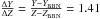
The 1σ internal uncertainties on the stellar parameters found with AME have been estimated by considering the centre and the corners of the relevant error box. For the mass, we considered the (Δν,Teff, [Fe /H]) error box whilst the error box applicable to the mean density and age was (Δν,M, [Fe/H]) in both cases. The 1σ uncertainties for the derived quantities (radius and surface gravity) were found in a similar manner, but taking the correlation between mass and mean density into account. (We recall that the mass was used to determine the mean density.) We describe below in some detail the determination of the mass uncertainty for α Cen A, and the other uncertainties follow by extension.
The values of the large separation, effective temperature, and metallicity and of their
associated error bars for α Cen A can be found in Table 2. Note that α Cen A is one of many stars in this paper where we
have inflated the Δν uncertainty to 1% in order to account for deviations from
the  scaling used for the large separations in the models.
We first fixed [Fe/H] at its centre value, [Fe/H] = +0.22 dex, and calculated the values of Teff · 100.09 · [Fe/H] and Δν · 10−0.05 · [Fe/H] (the axes in Fig. 3) using the values of Teff and Δν from Table 2, first without the 1σ uncertainties (the central value) and subsequently using Teff − σTeff and Teff + σTeff, as well as Δν − σΔν and Δν + σΔν. This gave us 6081 ± 52 K for the first expression and 102.9 ± 1.0 μHz for the second (see the first row of Table 3). From the central value (6081 K, 102.9 μHz), we estimated the central mass (1.10 M⊙ in this case) and from the possible combinations of the extreme values we did the same (6081−52 K and 102.9−1.0 μHz, 6081−52 K and 102.9 + 1.0 μHz, 6081 + 52 K and 102.9−1.0 μHz, and 6081 + 52 K and 102.9 + 1.0 μHz). To get the uncertainty on the central mass, we then took half of the full difference between the maximum and the minimum mass estimates obtained. This gave us a mass of 1.10 ± 0.02 M⊙, which can be seen in the right-hand column in the first row of Table 3.
After this, we calculated the values again using instead the +1σ and −1σ values of [Fe/H] in turn. The results can be seen in the last two rows of Table 3. The mass estimates and the associated errors from the uncertainties in Teff and Δν are given in the right-hand column.
To calculate the final 1σ uncertainty, we took half of the full difference
between the upper value mass estimate and the lower value
mass estimate given in Table 3. This we
added in quadrature (we assume the measurements to be independent) to the maximal
uncertainty on an individual mass estimate (to err on the side of caution). In the case of
α Cen A,
they are the same, 0.2
M⊙. We thus obtained a final mass and
uncertainty estimate of  (6)The result of
carrying out this operation for the other parameters of α Cen A can be found in
Sect. 5.
(6)The result of
carrying out this operation for the other parameters of α Cen A can be found in
Sect. 5.
It should be noted that we have confirmed that the uncertainties scale linearly, as could be expected. This means that using the 3σ error bars on the input parameters (Δν, Teff, and [Fe/H]) leads to an increase of a factor of ~3 in the uncertainties of the stellar mass, mean density, radius, surface gravity, and age.
5. Results
AME has been used on seven stars with known interferometric radii, 20 stars with radii based on parallaxes determined with the Hipparcos satellite, and 16 solar-like stars with results from detailed modelling (in some cases in combination with results from other approaches). The results from AME for these three groups of stars are presented in separate sections below.
5.1. Stars with interferometry
Literature and AME values for the seven stars with interferometric radii.
We used AME on seven stars with radii determined from interferometry and parallaxes. These seven stars are four of the stars from Huber et al. (2012) and the three stars θ Cyg, 16 Cyg A, and 16 Cyg B, which have interferometric radii found by White et al. (2013). A comparison of the AME results with those from interferometry allows us to assess the reliability of the radii from AME, since interferometric radii are among the most model-independent radii that can be obtained. The input parameters needed for AME for the seven stars are given in Table 4, along with the known interferometric radii and the radii obtained with AME. Figure 6 shows the fractional difference between the interferometric radius and the radius found from AME as a function of metallicity and effective temperature. By fractional difference we mean the difference between the interferometric radius and the AME radius divided by the AME radius.
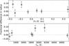 |
Fig. 6 Fractional difference in radius as a function of metallicity and effective temperature for the seven stars with radii determined from interferometry. The open symbols give the fractional difference between the stellar radius determined from interferometry and the one determined from AME (the ratio of the difference in radius and the radius from AME). The errors have been added in quadrature. The dashed line marks a fractional difference of zero. |
It is clear from Fig. 6 that the agreement between the AME and the interferometric radii is good. No trend is seen in the difference either as a function of metallicity or as a function of effective temperature, and the weighted mean of the fractional differences is just 1.7% (using as weights: w = 1/σ2 where σ denotes the size of the relevant error bar).
5.2. Stars with parallaxes
Literature and AME values for the 20 stars with radii based on parallaxes and angular diameters.
AME has been used on a sample of 20 stars from Silva Aguirre et al. (2012). These stars have radii determined from measurements of their parallaxes and calculations of their angular diameters (for details see Silva Aguirre et al. 2012). We wanted to use AME on these stars in order to facilitate a comparison between the reasonably model-independent radii from parallaxes and the ones from AME. Table 5 gives the relevant parameters from Silva Aguirre et al. (2012) for the 20 stars, as well as the radii returned by AME Four stars are in common between this sample and the interferometric sample (compare Table 5 to Table 4). In the middle panel of Figs. 7a and b we show the fractional difference between the parallax-based radius and the AME radius (again the ratio of the difference and the AME radius) as a function of metallicity and effective temperature.
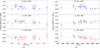 |
Fig. 7 Fractional difference in radius as a function of a) metallicity and b) effective temperature for the 20 stars with radii based on parallaxes. The symbols give the fractional difference between the stellar radius determined from the parallax (SA12), the stellar radius determined from AME, and the one determined using the BaSTI grid in turn. (We made the difference fractional by dividing it with the radius from AME.) The individual errors on the radii have been added in quadrature. The dashed line marks a difference of zero. |
Stellar parameters from AME for the 16 stars with properties determined from detailed modelling.
The agreement between the AME and the parallax-based radii is better than 2σ for all targets, and no clear slope is seen in the figures either as a function of effective temperature or as a function of metallicity. However, it is evident that the AME radii are generally smaller than the parallax ones, which can be seen as a positive offset in the plots. To look into this, we determined the radii for all the stars using the BaSTI grid of stellar models. It uses the same input parameters as AME and thus not the νmax scaling mentioned in Sect. 1.
Briefly, the BaSTI grid was originally computed for the Casagrande et al. (2011) revision of the Geneva-Copenhagen Survey and has now been extended in metallicity range for asteroseismic purposes. The input physics is as described in Pietrinferni et al. (2004), while the final stellar parameters are determined performing Monte Carlo simulations over the input parameters (Teff, [Fe/H], and Δν). The interested reader can find further details in Silva Aguirre et al. (2013).
The results of comparing these radii to the parallax-based and AME radii can be found in the top and bottom panels of Fig. 7. It can be seen that the fractional differences between the radii derived from the parallax and the BaSTI radii show distributions similar to the fractional differences between the parallax-based and AME radii. Comparison of the AME and BaSTI results (bottom panels) show that these agree better than the others. The AME-BaSTI plot only has four stars with a fractional difference in excess of 1σ, while this number is more than twice as high in the parallax-BaSTI and the parallax-AME plots. We return to the offset in Sect. 6.2.
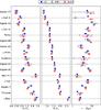 |
Fig. 8 Comparison of the mass, radius, and age values found using AME, in the literature (Lit), and using the BaSTI grid for the stars with parameters known from detailed modelling. The values and their error bars have been plotted. Where the error bars cannot be seen, they are smaller than the symbol used to plot the point except in the case of Kepler-37. Here, no uncertainty is quoted in the literature for its age, which is why this point has no error bar in the plot. |
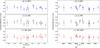 |
Fig. 9 Comparison of the difference in mass as a function of metallicity (panel a)) and effective temperature (panel b)) for the stars with results from detailed modelling. The different coloured points show the Lit-AME, Lit-BaSTI, and AME-BaSTI differences. The differences have been made fractional by dividing the difference with the mass obtained with AME. The errors have been added in quadrature. |
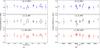 |
Fig. 10 Comparison of the difference in radius as a function of metallicity (panel a)) and effective temperature (panel b)) for Lit-AME, Lit-BaSTI, and AME-BaSTI. All the differences have been scaled with the AME radius, thus making the differences fractional. The errors have been added in quadrature. |
5.3. Stars with detailed modelling
AME has been used on 16 solar-like stars for which results from detailed modelling were available. As in the other cases, this allows for a comparison of the properties obtained from AME with those available in the literature, albeit in this case with parameters that are more model-dependent than the radii we compared to in the previous sections. However, it should be noted that α Cen A and B have their masses determined from their binarity and their radii from interferometry. Also, for the 16 stars with detailed modelling results, we compare not only the radii, but also the masses and ages. Table 6 lists the stellar parameters that were obtained with AME for the detailed modelling targets. (The literature values can be found in Table 2.)
To compare the output from AME with more than the parameters from detailed modelling, which are based on more information and have assumptions that vary from star to star, we also ran all stars through the BaSTI grid of stellar models. We did this to get a set of consistent results for all the stars based on inputs similar to AME. (For Perky and Dushera, the BaSTI results were taken from Silva Aguirre et al. 2013.)
Figure 8 shows a comparison between the mass, radius, and age results obtained with AME and those found in the literature (Table 2) and using the BaSTI grid. The age of Kepler-37 is given as ~6 Gyr by Barclay et al. (2013), and consequently no error bars on the age have been plotted in Fig. 8 for this star.
It can be seen from Fig. 8 that the stellar parameters found using AME are, in general, consistent with the parameters found in the literature and using the BaSTI grid. This is very satisfactory because it indicates that AME can be reliably used to determine stellar properties. Figures 9 and 10 show the fractional differences in mass and radius between two sets of results at a time (Lit-BaSTI, Lit-AME, and AME-BaSTI) as a function of metallicity and effective temperature. To make the differences fractional, they have all been scaled with the AME results.
Most of the stars fall at or below the 1σ level, which means that the results from the different methods generally agree quite well within their individual uncertainties. No trend or offset is apparent in either of the plots, and this is encouraging because it shows that AME can reproduce the BaSTI and detailed modelling results without any bias. Also, it is noteworthy that the groups of points Lit-BaSTI and Lit-AME show similar distributions. This implies that the AME and BaSTI results agree equally well with the literature. Furthermore, the AME and the BaSTI set of results also agree well with each other. It is reassuring that AME can produce results that are similar to the BaSTI results since AME and BaSTI use similar amounts of information as input for their results. In summary, we find that the masses and radii from AME and BaSTI agree very well, signifying that our method is at the same level as a grid-based approach.
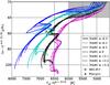 |
Fig. 11 Plot used to determine the mass for high mass stars. The different line colours signify the masses of the lines ranging from 1.3 M⊙ (magenta/purple) to 1.6 M⊙ (blue) in steps of 0.1 M⊙. The various line types indicate the metallicity. The shaded area shows where the lines start to become hard to separate. The yellow star indicates the position of HAT-P-7 whilst the red star gives the location of Procyon in the plot. |
A few of the results given in Table 6 deserve further comment. In the case of Procyon, this star was found to be placed in an area of the mass plot where lines of different masses cross (see Fig. 11). The reason for this crossing is the MS turn-off. Since a star passes through this phase relatively fast compared to its MS and sub-giant-branch lifetimes (for our models, the evolution of a 1.4 M⊙ star in the turn-off phase is more than twice as fast as in the MS phase and approximately 20% faster than in the sub-giant phase), we assumed that Procyon was not in the turn-off, so we disregarded those lines (the 1.5 M⊙ lines) when we determined its mass. As a consequence of this, for stars in some parts of the plots, systematic differences could occur due to the non-negligible possibility of being in a different evolutionary phase. A similar assumption to the case Procyon was made for HAT-P-7. Here, we chose to use tracks that were in the same evolutionary state for determining the mass (see Fig. 11). This meant that we used the pre-turn-off tracks (1.5 M⊙ and 1.6 M⊙ tracks) to establish the mass and thus ignored the 1.4 M⊙ lines in this case.
We also had to ignore some of the lines when we determined the masses of two of the parallax stars from Table 5. These two stars are KIC5371516 and KIC9139151. For the former, it was situated right on top of the 1.5 M⊙ MS turn-off tracks seen in Fig. 11, and as a consequence, we chose to determine its mass via linear extrapolation based on the 1.3 M⊙ and 1.4 M⊙ tracks that were in the same evolutionary state at the location of the star. For the latter star, the situation was a little different, since it was not located near the MS turn-off, but instead in the bottom part of the mass plot for low-mass stars seen in Fig. 3 before the beginning of the 1.3 M⊙ tracks. Probably as an effect of the density of the grid, the mass of this star needed to be determined by extrapolation based on the 1.1 M⊙ and 1.2 M⊙ tracks. Had the grid been denser such that a track had been present for a 1.25 M⊙ star, this extrapolation would probably not have been necessary. (The mass of the star was found to be 1.23 M⊙.)
As can be seen when inspecting Tables 2 and 4, a few of the metallicity values lie slightly beyond the AME grid. In these cases, we used linear extrapolation similar to what was described above. Great care was taken to make sure that the results were meaningful: they have been manually inspected, and we did not attempt metallicities that were far from the grid.
It can happen that a star falls close to the limit of a plot. For instance, the star Perky has a metallicity of −0.09 ± 0.1 dex, which means that when the uncertainties were considered, two different plots had to be used to estimate the mean density and its associated error bar. (The same was true for the age.) In this case, we simply used the relevant plot according to the corner of the error box under consideration.
It may also occur that a star falls exactly on the limit between two plots, which is the case for the star KIC3733735 (see Table 5) since it has a metallicity of −0.10 ± 0.1 dex. For it, we used both relevant plots to determine the mean density and used the plot with the appropriate metallicity depending on the corner of the error box to find the uncertainty. The plots used to establish the mean density returned identical results. (Again, the same was true for the age.) If this had not been the case, we would have used the mean value as the result and added the difference between the plots in quadrature to the uncertainty estimates.
6. Discussion
We comment on the results from studying the seven stars with radii from interferometry in Sect. 6.1, the results for the 20 stars with radii based on measurements of their parallaxes in Sect. 6.2, and finally the results for the 16 targets with results from detailed modelling in Sect. 6.3.
6.1. Stars with interferometry
The agreement between the interferometric and AME radii is excellent, as can be seen from Fig. 6. Five of the seven stars have results that are within 1σ, while two stars have radii that differ by more than 1σ (2.0σ and 2.2σ, respectively). These two stars are KIC6106415 and KIC6225718, and they have the smallest angular diameters of the stars measured by Huber et al. (2012). Thus, their interferometric uncertainties are more difficult to determine than those for the stars with larger angular diameters. The weighted mean of the fractional differences between the interferometric and the AME radii is 1.7%, as mentioned earlier. As a result, the radii from AME are consistent with the interferometric radii over the range of metallicities, effective temperatures, and large separations represented by the interferometric targets. The consistency between the AME and the largely model-independent interferometric radii implies that the radii from AME are probably trustworthy and accurate.
6.2. Stars with parallaxes
The offset seen in Fig. 7 points towards a systematic difference between the radii given in the literature for the parallax stars (SA12 radii) and the AME radii. In spite of the offset, the radii from AME are still within 5% of the SA12 radii, which is the accuracy claimed by Silva Aguirre et al. (2012). In fact the weighted mean of the fractional differences is 2.3%. The weighted mean of the fractional differences when comparing the SA12 results to the BaSTI results is 2.1%, which is similar to the SA12-AME value, while the AME-BaSTI weighted mean of the fractional differences is 1.4%. Thus SA12-AME radii and SA12-BaSTI radii show similar discrepancies while the AME-BaSTI radii agree slightly better.
A similar offset to the one seen between SA12 and AME, and SA12 and BaSTI in Fig. 7b, both in size and shape, is found by Chaplin et al. (2014) (see the top left panel of their Fig. 4). They
find that the “boomerang” shaped discrepancy arises from the difference between
determining Δν from individual oscillation frequencies and from
the
scaling relation. We use a similar approach to the scaling relation approach to find the
large separation for the models in AME (we use the sound-speed integral given in Eq.
(2)), and the approach for the stars in
Silva Aguirre et al. (2012) is to use calculated
oscillations frequencies to obtain the large separation. As a consequence, a similar
discrepancy can be expected – and found – for our comparison of the SA12 and the AME
results. (Chaplin et al. 2014 plot the fractional
difference in the “scaling relation-individual” sense where we have done the opposite and
their temperature axis is reversed with respect to ours.) BaSTI finds the large separation
of its models using the scaling relation, and as a consequence the same boomerang is also
expected – and seen – for the SA12 – BaSTI comparison (see the top panel of Fig. 7b). However, the shape and size of the offset in the case of
SA12-AME is not completely the same as the SA12-BaSTI one. This may be because we do not
use the exact same method to find the Δν’s, as mentioned before. From Fig. 7b it appears that using the sound-speed integral to find the
large separation (and scaling it as we have done) introduces a smaller offset than using
the scaling relation to obtain it (as BaSTI does). For the warmest stars, we see the
deviation in shape between the SA12-AME and the SA12-BaSTI results. There is an indication
that the AME radii are underestimated for these warmest stars. However, these stars are F
stars first of all and therefore notoriously challenging. And second, AME uses scaling to
the Sun, but these stars are the least Sun-like in the sample, so it makes sense that the
AME results show a small discrepancy from the SA12 results.
6.3. Stars with detailed modelling
From Fig. 8 and Table 6 it is seen that the AME ages generally have fairly large error bars. The age values that have been found for the stars with detailed modelling have a median uncertainty of 25% (with percentages ranging from 12% to 173%), while the median uncertainty on the mass of these stars is 4%, and the median uncertainty on the radius for the full sample of stars is 2%. However, to be able to determine the age was not an initial goal of AME, and the reason for the sometimes quite large error bars on the AME age determinations is largely the strong dependence of the age on the mass (see the y axis of Fig. 5). Note that the median uncertainties are internal uncertainties, and as a consequence systematic errors arising from, for instance, the chosen input physics are not taken into account.
Furthermore, the ages are the plotted AME parameter in Fig. 8 that differ most from the literature and BaSTI properties. The weighted mean of the fractional differences between the literature and AME ages is 15%, whilst it is 10% between the AME and the BaSTI ages. This is of course a large difference, but still the AME ages can be used as estimates, especially when one considers the uncertainties, since the ages from AME are most often within 1σ of the BaSTI and the literature values. The star α Cen B is a noticeable example of a star whose age differs by more than 1σ from the value given in the literature. The reason for this deviation and the large uncertainty is probably a combination of its early evolutionary state (which places it where the curve on the graph in Fig. 5 is steep) and the fact that the mass deviates by 1σ from the one given in the literature. (The mass has a high exponent on the y axis of the age plot.) The mass that AME finds is higher than the literature one, so the age will be underestimated.
In Fig. 8 the masses and radii from AME agree well with the values from the other sources. Since these parameters are more precisely determined than the age in results from AME, the literature, and BaSTI, we have taken a closer look at these parameters by plotting them as functions of metallicity and effective temperature in Figs. 9 and 10.
There are a few outliers in the Lit-AME group that can be seen if we consider the middle panels of these figures. In the middle panels of Fig. 9, four stars have masses that differ by more than 1σ. These are Kepler-10, Procyon, Kepler-7, and μ Arae. However, the weighted mean of the fractional differences of all the masses is just 4%, and only Kepler-7 has a mass value that differs by more than 2σ.
Figures 10a and 10b show the radius differences as a function of metallicity and effective temperature, respectively. The weighted mean of the fractional differences between the literature and the AME results (middle panels) is only 1.3%, but there are still four stars with a fractional difference in excess of 1σ. These are α Cen B and the three sub-giants β Hyi, Procyon, and η Boo. We have already discussed α Cen B, so we focus on the sub-giants now. A possible explanation for the trend that the results for the sub-giants deviate by more than 1σ is that the temperature sensitivity of the AME results for the sub-giants is a lot higher than for stars on the MS. (See Fig. 2 where it is clear that the evolution tracks of models with different masses lie a lot closer at low Δν than at high values of Δν.) It is noteworthy that the BaSTI and AME results for Procyon agree closely (better than 1σ) and that the agreement between the BaSTI and AME results for β Hyi and η Boo is also good (the fractional difference is just above 1σ in both cases).
The bottom panels of Figs. 9 and 10 show the fractional differences between the AME and BaSTI results. The agreement between the results is good. The weighted mean of the fractional differences is 4% in mass and 1.6% in radius. Only a couple of stars have fractional differences in excess of 1σ and all of these deviate by less than 2σ. For the mass differences, the stars that deviate by more than 1σ are Kepler-10, Kepler-68, α Cen B, and μ Arae, while the ones that differ by more than 1σ in radius are Kepler-68, α Cen B, and μ Arae, as in the mass case, and then the two sub-giants β Hyi and η Boo. Considering the low weighted mean of the fractional differences, the results are very promising since AME and the BaSTI grid obtain their stellar properties based on a similar amount of information. All in all, AME displays good agreement with both results from the BaSTI grid and values found in the literature. This goes on to show that AME can be reliably used to obtain basic stellar parameters for stars exhibiting solar-like oscillations.
7. Conclusion
We have shown that as a tool to determine basic stellar parameters, AME works very well. It offers a transparent and easy way to find stellar properties for stars exhibiting solar-like oscillations at a level where the large separation can be detected. The full set of AME figures that are the backbone of the method can be found in the online material appendix A. They cover a range in masses from 0.7 M⊙ in steps of 0.1 M⊙ to 1.6 M⊙, and in metallicity the span is −0.3 dex ≤ [Fe/H] ≤ +0.3 dex in increments of 0.1 dex.
We used AME on a total of 43 stars with stellar parameters determined in different ways. We compared the results from AME to those found in the literature and, in some cases, to results obtained with the BaSTI grid. The overall agreement is good, and the differences can be explained. AME was found to perform as well as the BaSTI grid in terms of agreement with the values quoted in the literature for the 16 stars with results from detailed modelling. Furthermore, the radii from AME was found to be consistent with both radii from interferometry (and measured parallaxes) and radii determined from parallaxes (and computed angular diameters).
In the future, the AME grid will be extended to cover a wider range of metallicities and masses and potentially made denser. We are currently working on a web interface to enable people to use AME without having to plot their stars in the diagrams themselves.
Colour-mass correspondence in the AME figures.
Calculated from the MESA values of the gravitational constant, the solar mass, and the solar radius.
Acknowledgments
Funding for the Stellar Astrophysics Centre is provided by The Danish National Research Foundation (Grant agreement No.: DNRF106). The research is supported by the ASTERISK project (ASTERoseismic Investigations with SONG and Kepler) funded by the European Research Council (Grant agreement No.: 267864).
References
- Aerts, C., Christensen-Dalsgaard, J., & Kurtz, D. W. 2010, Asteroseismology, 1st edn. (Springer) [Google Scholar]
- Angulo, C., Arnould, M., Rayet, M., et al. 1999, Nucl. Phys. A, 656, 3 [NASA ADS] [CrossRef] [Google Scholar]
- Asplund, M., Grevesse, N., Sauval, A. J., & Scott, P. 2009, Ann. Rev. Astron. Astrophys., 47, 481 [CrossRef] [Google Scholar]
- Balser, D. S. 2006, AJ, 132, 2326 [NASA ADS] [CrossRef] [Google Scholar]
- Barclay, T., Rowe, J. F., Lissauer, J. J., et al. 2013, Nature, 494, 452 [NASA ADS] [CrossRef] [Google Scholar]
- Basu, S., Chaplin, W. J., & Elsworth, Y. 2010, ApJ, 710, 1596 [NASA ADS] [CrossRef] [Google Scholar]
- Batalha, N. M., Borucki, W. J., Bryson, S. T., et al. 2011, ApJ, 729, 27 [NASA ADS] [CrossRef] [Google Scholar]
- Bedding, T. R., & Kjeldsen, H. 2010, Commun. Asteroseismol., 161, 3 [NASA ADS] [CrossRef] [Google Scholar]
- Bedding, T. R., Kjeldsen, H., Arentoft, T., et al. 2007, ApJ, 663, 1315 [NASA ADS] [CrossRef] [Google Scholar]
- Bedding, T. R., Kjeldsen, H., Campante, T. L., et al. 2010, ApJ, 713, 935 [NASA ADS] [CrossRef] [Google Scholar]
- Belkacem, K., Goupil, M. J., Dupret, M. A., et al. 2011, A&A, 530, A142 [NASA ADS] [CrossRef] [EDP Sciences] [Google Scholar]
- Belkacem, K., Samadi, R., Mosser, B., Goupil, M. J., & Ludwig, H.-G. 2013, ASP Conf. Proc., 479, 61 [Google Scholar]
- Böhm-Vitense, E. 1958, ZAp, 46, 108 [NASA ADS] [Google Scholar]
- Bonaca, A., Tanner, J. D., Basu, S., et al. 2012, ApJ, 755, L12 [NASA ADS] [CrossRef] [Google Scholar]
- Bouchy, F., & Carrier, F. 2002, A&A, 390, 205 [NASA ADS] [CrossRef] [EDP Sciences] [Google Scholar]
- Brandão, I. M., Doğan, G., Christensen-Dalsgaard, J., et al. 2011, A&A, 527, A37 [NASA ADS] [CrossRef] [EDP Sciences] [Google Scholar]
- Bruntt, H., Bedding, T. R., Quirion, P.-O., et al. 2010, MNRAS, 405, 1907 [NASA ADS] [Google Scholar]
- Bruntt, H., Basu, S., Smalley, B., et al. 2012, MNRAS, 423, 122 [NASA ADS] [CrossRef] [Google Scholar]
- Carrier, F., & Bourban, G. 2003, A&A, 406, L23 [NASA ADS] [CrossRef] [EDP Sciences] [Google Scholar]
- Carrier, F., Eggenberger, P., & Bouchy, F. 2005, A&A, 434, 1085 [NASA ADS] [CrossRef] [EDP Sciences] [Google Scholar]
- Carter, J. A., Agol, E., Chaplin, W. J., et al. 2012, Science, 337, 556 [NASA ADS] [CrossRef] [PubMed] [Google Scholar]
- Casagrande, L., Schönrich, R., Asplund, M., et al. 2011, A&A, 530, A138 [NASA ADS] [CrossRef] [EDP Sciences] [Google Scholar]
- Chaplin, W. J., & Miglio, A. 2013, ARA&A, 51, 353 [NASA ADS] [CrossRef] [Google Scholar]
- Chaplin, W. J., Kjeldsen, H., Christensen-Dalsgaard, J., et al. 2011, Science, 332, 213 [NASA ADS] [CrossRef] [PubMed] [Google Scholar]
- Chaplin, W. J., Sanchis-Ojeda, R., Campante, T. L., et al. 2013, A&A, 766, A101 [NASA ADS] [CrossRef] [EDP Sciences] [Google Scholar]
- Chaplin, W. J., Basu, S., Huber, D., et al. 2014, ApJS, 210, 1 [NASA ADS] [CrossRef] [Google Scholar]
- Christensen-Dalsgaard, J. 2008, Ap&SS, 316, 13 [NASA ADS] [CrossRef] [Google Scholar]
- Christensen-Dalsgaard, J., & Houdek, G. 2010, Ap&SS, 328, 51 [NASA ADS] [CrossRef] [Google Scholar]
- Demory, B.-O., Seager, S., Madhusudhan, N., et al. 2011, ApJ, 735, L12 [NASA ADS] [CrossRef] [Google Scholar]
- Eggenberger, P., Charbonnel, C., Talon, S., et al. 2004, A&A, 417, 235 [NASA ADS] [CrossRef] [EDP Sciences] [Google Scholar]
- Erspamer, D., & North, P. 2003, A&A, 398, 1121 [NASA ADS] [CrossRef] [EDP Sciences] [Google Scholar]
- Ferguson, J. W., Alexander, D. R., Allard, F., et al. 2005, ApJ, 623, 585 [NASA ADS] [CrossRef] [Google Scholar]
- Fogtmann-Schulz, A., Hinrup, B., Van Eylen, V., et al. 2014, ApJ, 781, 67 [NASA ADS] [CrossRef] [Google Scholar]
- Formicola, A., Imbriani, G., Costantini, H., et al. 2004, Phys. Lett. B, 591, 61 [NASA ADS] [CrossRef] [Google Scholar]
- Gai, N., Basu, S., Chaplin, W. J., & Elsworth, Y. 2011, ApJ, 730, 63 [NASA ADS] [CrossRef] [Google Scholar]
- Gilliland, R. L., Marcy, G. W., Rowe, J. F., et al. 2013, ApJ, 766, 40 [NASA ADS] [CrossRef] [Google Scholar]
- Grevesse, N., & Sauval, A. J. 1998, Space Sci. Rev., 85, 161 [NASA ADS] [CrossRef] [Google Scholar]
- Guzik, J. A., Houdek, G., Chaplin, W. J., et al. 2011 [arXiv:1110.2120] [Google Scholar]
- Hansen, C. J., Kawaler, S. D., & Trimble, V. 2004, Stellar interiors: physical principles, structure, and evolution [Google Scholar]
- Huber, D., Ireland, M. J., Bedding, T. R., et al. 2012, ApJ, 760, 32 [NASA ADS] [CrossRef] [Google Scholar]
- Huber, D., Chaplin, W. J., Christensen-Dalsgaard, J., et al. 2013, ApJ, 767, 127 [NASA ADS] [CrossRef] [Google Scholar]
- Iglesias, C. A., & Rogers, F. J. 1996, ApJ, 464, 943 [NASA ADS] [CrossRef] [Google Scholar]
- Kervella, P., Thévenin, F., Ségransan, D., et al. 2003, A&A, 404, 1087 [NASA ADS] [CrossRef] [EDP Sciences] [Google Scholar]
- Kippenhahn, R., Weigert, A., & Weiss, A. 2013, Stellar Structure and Evolution Astron. Astrophys. Lib. (Heidelberg, Berlin: Springer-Verlag) [Google Scholar]
- Kjeldsen, H., & Bedding, T. R. 1995, A&A, 293, 87 [NASA ADS] [Google Scholar]
- Kjeldsen, H., Bedding, T. R., & Christensen-Dalsgaard, J. 2008, ApJ, 683, L175 [NASA ADS] [CrossRef] [Google Scholar]
- Koch, D. G., Borucki, W. J., Basri, G., et al. 2010, ApJ, 713, L79 [NASA ADS] [CrossRef] [Google Scholar]
- Latham, D. W., Borucki, W. J., Koch, D. G., et al. 2010, ApJ, 713, L140 [NASA ADS] [CrossRef] [Google Scholar]
- Liebert, J., Fontaine, G., Young, P. A., Williams, K. A., & Arnett, D. 2013, ApJ, 769, 7 [NASA ADS] [CrossRef] [Google Scholar]
- Mathur, S., García, R. A., Régulo, C., et al. 2010, A&A, 511, A46 [NASA ADS] [CrossRef] [EDP Sciences] [Google Scholar]
- Pál, A., Bakos, G. Á., Torres, G., et al. 2008, ApJ, 680, 1450 [NASA ADS] [CrossRef] [Google Scholar]
- Paxton, B., Bildsten, L., Dotter, A., et al. 2011, ApJS, 192, 3 [Google Scholar]
- Paxton, B., Cantiello, M., Arras, P., et al. 2013, ApJS, 208, 4 [NASA ADS] [CrossRef] [Google Scholar]
- Pietrinferni, A., Cassisi, S., Salaris, M., & Castelli, F. 2004, ApJ, 612, 168 [NASA ADS] [CrossRef] [Google Scholar]
- Pourbaix, D., Nidever, D., McCarthy, C., et al. 2002, A&A, 386, 280 [NASA ADS] [CrossRef] [EDP Sciences] [Google Scholar]
- Quirion, P.-O., Christensen-Dalsgaard, J., & Arentoft, T. 2010, ApJ, 725, 2176 [NASA ADS] [CrossRef] [Google Scholar]
- Ramírez, I., Meléndez, J., & Asplund, M. 2009, A&A, 508, L17 [NASA ADS] [CrossRef] [EDP Sciences] [Google Scholar]
- Rogers, F. J., & Nayfonov, A. 2002, ApJ, 576, 1064 [Google Scholar]
- Rogers, F. J., Swenson, F. J., & Iglesias, C. A. 1996, ApJ, 456, 902 [NASA ADS] [CrossRef] [Google Scholar]
- Santos, N. C., Bouchy, F., Mayor, M., et al. 2004, A&A, 426, L19 [NASA ADS] [CrossRef] [EDP Sciences] [Google Scholar]
- Silva Aguirre, V., Ballot, J., Serenelli, A. M., & Weiss, A. 2011, A&A, 529, A63 [NASA ADS] [CrossRef] [EDP Sciences] [Google Scholar]
- SilvaAguirre, V., Casagrande, L., Basu, S., et al. 2012, ApJ, 757, 99 [NASA ADS] [CrossRef] [Google Scholar]
- SilvaAguirre, V., Basu, S., Brandão, I. M., et al. 2013, ApJ, 769, 141 [NASA ADS] [CrossRef] [Google Scholar]
- Soriano, M., & Vauclair, S. 2010, A&A, 513, A49 [NASA ADS] [CrossRef] [EDP Sciences] [Google Scholar]
- Steigman, G. 2010, J. Cosmol. Astropart. Phys., 4, 29 [Google Scholar]
- Stello, D., Chaplin, W. J., Basu, S., Elsworth, Y., & Bedding, T. R. 2009a, MNRAS, 400, L80 [NASA ADS] [CrossRef] [Google Scholar]
- Stello, D., Chaplin, W. J., Bruntt, H., et al. 2009b, ApJ, 700, 1589 [NASA ADS] [CrossRef] [Google Scholar]
- Torres, G., Fischer, D. A., Sozzetti, A., et al. 2012, ApJ, 757, 161 [NASA ADS] [CrossRef] [Google Scholar]
- Toutain, T., & Fröhlich, C. 1992, A&A, 257, 287 [NASA ADS] [Google Scholar]
- Turcotte, S., Richer, J., & Michaud, G. 1998, ApJ, 504, 559 [NASA ADS] [CrossRef] [Google Scholar]
- Valle, G., Dell’Omodarme, M., Prada Moroni, P. G., & Degl’Innocenti, S. 2014, A&A, 561, A125 [NASA ADS] [CrossRef] [EDP Sciences] [Google Scholar]
- Weiss, A., & Schlattl, H. 2008, Ap&SS, 316, 99 [NASA ADS] [CrossRef] [Google Scholar]
- White, T. R., Bedding, T. R., Stello, D., et al. 2011a, ApJ, 742, L3 [NASA ADS] [CrossRef] [Google Scholar]
- White, T. R., Bedding, T. R., Stello, D., et al. 2011b, ApJ, 743, 161 [NASA ADS] [CrossRef] [Google Scholar]
- White, T. R., Huber, D., Maestro, V., et al. 2013, MNRAS, 433, 1262 [NASA ADS] [CrossRef] [Google Scholar]
Appendix A: All AME figures
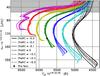 |
Fig. A.1 Plot for determining the stellar mass. The colours give the masses of the lines ranging from 0.7 M⊙ (black) in steps of 0.1 M⊙ to 1.3 M⊙ (magenta/purple). The different line types are explained in the legend. The star shows the location of the Sun in the figure. The shaded area in the top of the figure indicates the region where Fig. A.2 should be used instead. |
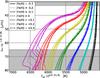 |
Fig. A.2 Plot for determining the stellar mass. The colours give the masses of the lines ranging from 0.7 M⊙ (black) in steps of 0.1 M⊙ to 1.3 M⊙ (magenta/purple). The different line types are explained in the legend. The shaded areas in the figure indicate where Fig. A.1 should be used instead (bottom) and where the lines are hard to disentangle (top). |
In this appendix we provide the full set of AME figures. Section A.1 contains the three mass plots, the six mean-density plots are given in Sects. A.2, and A.3 holds the six age plots.
Explanations of the figures are given in the main text, and the figure captions provide the information needed to use the figures. An overview of which colour corresponds to which mass is provided in Table A.1 below.
Appendix A.1: Mass plots
Figures A.1–A.3 show the plots that can be used to determine the stellar mass.
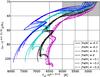 |
Fig. A.3 Plot for determining the stellar mass. The colours give the masses of the lines ranging from 1.3 M⊙ (magenta/purple) in steps of 0.1 M⊙ to 1.6 M⊙ (blue). The different line types are explained in the legend. The shaded area in the figure indicates where the lines are hard to disentangle. In the middle of the plot, where the tracks mix (ordinate values of ~60 μHz), is where a star will go through the MS turn-off. |
Appendix A.2: Mean-density plots
Figures A.4 to A.9 show the plots that can be used to obtain the stellar mean density.
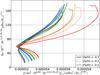 |
Fig. A.4 Plot for determining the stellar mean density for stars with −0.30 dex ≤ [Fe/H] ≤ −0.10 dex. The colours give the masses of the lines ranging from 0.7 M⊙ (black) in steps of 0.1 M⊙ to 1.2 M⊙ (red). The different line types are explained in the legend. |
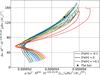 |
Fig. A.5 Plot for determining the stellar mean density for stars with −0.10 dex ≤ [Fe/H] ≤ +0.10 dex. The colours give the masses of the lines ranging from 0.7 M⊙ (black) in steps of 0.1 M⊙ to 1.2 M⊙ (red). The different line types are explained in the legend. The star indicates the position of the Sun. |
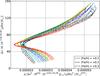 |
Fig. A.6 Plot for determining the stellar mean density for stars with +0.10 dex ≤ [Fe/H] ≤ +0.30 dex. The colours give the masses of the lines ranging from 0.7 M⊙ (black) in steps of 0.1 M⊙ to 1.2 M⊙ (red). The different line types are explained in the legend. |
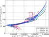 |
Fig. A.7 Plot for determining the stellar mean density for stars with −0.30 dex ≤ [Fe/H] ≤ −0.10 dex. The colours give the masses of the lines ranging from 1.2 M⊙ (red) in steps of 0.1 M⊙ to 1.6 M⊙ (blue). The different line types are explained in the legend. |
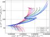 |
Fig. A.8 Plot for determining the stellar mean density for stars with −0.10 dex ≤ [Fe/H] ≤ +0.10 dex. The colours give the masses of the lines ranging from 1.2 M⊙ (red) in steps of 0.1 M⊙ to 1.6 M⊙ (blue). The different line types are explained in the legend. |
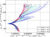 |
Fig. A.9 Plot for determining the stellar mean density for stars with +0.10 dex ≤ [Fe/H] ≤ +0.30 dex. The colours give the masses of the lines ranging from 1.2 M⊙ (red) in steps of 0.1 M⊙ to 1.6 M⊙ (blue). The different line types are explained in the legend. |
Appendix A.3: Age plots
Figures A.10 to A.15 give the plots that can be used to estimate the stellar age.
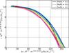 |
Fig. A.10 Plot for determining the stellar age for stars with −0.30 dex ≤ [Fe/H] ≤ −0.10 dex. The colours give the masses of the lines ranging from 0.7 M⊙ (black) in steps of 0.1 M⊙ to 1.3 M⊙ (magenta/purple). The different line types are explained in the legend. |
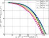 |
Fig. A.11 Plot for determining the stellar age for stars with −0.10 dex ≤ [Fe/H] ≤ +0.10 dex. The colours give the masses of the lines ranging from 0.7 M⊙ (black) in steps of 0.1 M⊙ to 1.3 M⊙ (magenta/purple). The different line types are explained in the legend. The star shows the location of the Sun. |
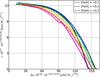 |
Fig. A.12 Plot for determining the stellar age for stars with +0.10 dex ≤ [Fe/H] ≤ +0.30 dex. The colours give the masses of the lines ranging from 0.7 M⊙ (black) in steps of 0.1 M⊙ to 1.3 M⊙ (magenta/purple). The different line types are explained in the legend. |
 |
Fig. A.13 Plot for determining the stellar age for stars with −0.30 dex ≤ [Fe/H] ≤ −0.10 dex. The colours give the masses of the lines ranging from 1.3 M⊙ (magenta/purple) in steps of 0.1 M⊙ to 1.6 M⊙ (blue). The different line types are explained in the legend. |
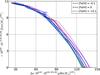 |
Fig. A.14 Plot for determining the stellar age for stars with −0.10 dex ≤ [Fe/H] ≤ +0.10 dex. The colours give the masses of the lines ranging from 1.3 M⊙ (magenta/purple) in steps of 0.1 M⊙ to 1.6 M⊙ (blue). The different line types are explained in the legend. |
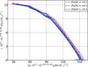 |
Fig. A.15 Plot for determining the stellar age for stars with +0.10 dex ≤ [Fe/H] ≤ +0.30 dex. The colours give the masses of the lines ranging from 1.3 M⊙ (magenta/purple) in steps of 0.1 M⊙ to 1.6 M⊙ (blue). The different line types are explained in the legend. |
All Tables
Literature and AME values for the 20 stars with radii based on parallaxes and angular diameters.
Stellar parameters from AME for the 16 stars with properties determined from detailed modelling.
All Figures
|
Fig. 1 H-R diagram comparing evolution tracks made with MESA, ASTEC, and GARSTEC for stars of mass 1.0 M⊙ and 1.2 M⊙ with two different chemical compositions: GS98 and A09. The star is the Sun. |
| In the text | |
|
Fig. 2 Evolutionary tracks for models with varying mass and solar metallicity plotted in a variation of a classic H-R diagram (Δν plotted against Teff). The star shows the location of the Sun and the different line colours represent different masses starting with the black 0.7 M⊙ line on the far right going in increments of 0.1 M⊙ to the blue 1.6 M⊙ line on the far left. |
| In the text | |
|
Fig. 3 Plot used to determine the mass of α Cen A. The colours give the masses of the lines ranging from 0.7 M⊙ (black) in the right of the figure in steps of 0.1 M⊙ to 1.3 M⊙ (magenta/purple) in the left of the figure. The different line types give the metallicity. The star shows the location of α Cen A in the figure. The shaded area in the top indicates the region where another mass plot would be more suitable. |
| In the text | |
|
Fig. 4 Plot used to determine the mean density of α Cen A. The colours represent different masses: 0.7 M⊙ (black), 0.8 M⊙ (light blue), 0.9 M⊙ (blue), 1.0 M⊙ (green), 1.1 M⊙ (yellow), and 1.2 M⊙ (red), whilst the line styles give the metallicity of a given line. The location of α Cen A in the plot is marked by the horizontal, black, dashed line. |
| In the text | |
|
Fig. 5 Plot used to determine the age of α Cen A. The colours represent different masses: 0.7 M⊙ (black), 0.8 M⊙ (light blue), 0.9 M⊙ (blue), 1.0 M⊙ (green), 1.1 M⊙ (yellow) 1.2 M⊙ (red), and 1.3 M⊙ (magenta/purple), whilst the line types indicate the metallicity of a given line. The location of α Cen A in the plot is marked by the vertical, black, dashed line. |
| In the text | |
|
Fig. 6 Fractional difference in radius as a function of metallicity and effective temperature for the seven stars with radii determined from interferometry. The open symbols give the fractional difference between the stellar radius determined from interferometry and the one determined from AME (the ratio of the difference in radius and the radius from AME). The errors have been added in quadrature. The dashed line marks a fractional difference of zero. |
| In the text | |
|
Fig. 7 Fractional difference in radius as a function of a) metallicity and b) effective temperature for the 20 stars with radii based on parallaxes. The symbols give the fractional difference between the stellar radius determined from the parallax (SA12), the stellar radius determined from AME, and the one determined using the BaSTI grid in turn. (We made the difference fractional by dividing it with the radius from AME.) The individual errors on the radii have been added in quadrature. The dashed line marks a difference of zero. |
| In the text | |
|
Fig. 8 Comparison of the mass, radius, and age values found using AME, in the literature (Lit), and using the BaSTI grid for the stars with parameters known from detailed modelling. The values and their error bars have been plotted. Where the error bars cannot be seen, they are smaller than the symbol used to plot the point except in the case of Kepler-37. Here, no uncertainty is quoted in the literature for its age, which is why this point has no error bar in the plot. |
| In the text | |
|
Fig. 9 Comparison of the difference in mass as a function of metallicity (panel a)) and effective temperature (panel b)) for the stars with results from detailed modelling. The different coloured points show the Lit-AME, Lit-BaSTI, and AME-BaSTI differences. The differences have been made fractional by dividing the difference with the mass obtained with AME. The errors have been added in quadrature. |
| In the text | |
|
Fig. 10 Comparison of the difference in radius as a function of metallicity (panel a)) and effective temperature (panel b)) for Lit-AME, Lit-BaSTI, and AME-BaSTI. All the differences have been scaled with the AME radius, thus making the differences fractional. The errors have been added in quadrature. |
| In the text | |
|
Fig. 11 Plot used to determine the mass for high mass stars. The different line colours signify the masses of the lines ranging from 1.3 M⊙ (magenta/purple) to 1.6 M⊙ (blue) in steps of 0.1 M⊙. The various line types indicate the metallicity. The shaded area shows where the lines start to become hard to separate. The yellow star indicates the position of HAT-P-7 whilst the red star gives the location of Procyon in the plot. |
| In the text | |
|
Fig. A.1 Plot for determining the stellar mass. The colours give the masses of the lines ranging from 0.7 M⊙ (black) in steps of 0.1 M⊙ to 1.3 M⊙ (magenta/purple). The different line types are explained in the legend. The star shows the location of the Sun in the figure. The shaded area in the top of the figure indicates the region where Fig. A.2 should be used instead. |
| In the text | |
|
Fig. A.2 Plot for determining the stellar mass. The colours give the masses of the lines ranging from 0.7 M⊙ (black) in steps of 0.1 M⊙ to 1.3 M⊙ (magenta/purple). The different line types are explained in the legend. The shaded areas in the figure indicate where Fig. A.1 should be used instead (bottom) and where the lines are hard to disentangle (top). |
| In the text | |
|
Fig. A.3 Plot for determining the stellar mass. The colours give the masses of the lines ranging from 1.3 M⊙ (magenta/purple) in steps of 0.1 M⊙ to 1.6 M⊙ (blue). The different line types are explained in the legend. The shaded area in the figure indicates where the lines are hard to disentangle. In the middle of the plot, where the tracks mix (ordinate values of ~60 μHz), is where a star will go through the MS turn-off. |
| In the text | |
|
Fig. A.4 Plot for determining the stellar mean density for stars with −0.30 dex ≤ [Fe/H] ≤ −0.10 dex. The colours give the masses of the lines ranging from 0.7 M⊙ (black) in steps of 0.1 M⊙ to 1.2 M⊙ (red). The different line types are explained in the legend. |
| In the text | |
|
Fig. A.5 Plot for determining the stellar mean density for stars with −0.10 dex ≤ [Fe/H] ≤ +0.10 dex. The colours give the masses of the lines ranging from 0.7 M⊙ (black) in steps of 0.1 M⊙ to 1.2 M⊙ (red). The different line types are explained in the legend. The star indicates the position of the Sun. |
| In the text | |
|
Fig. A.6 Plot for determining the stellar mean density for stars with +0.10 dex ≤ [Fe/H] ≤ +0.30 dex. The colours give the masses of the lines ranging from 0.7 M⊙ (black) in steps of 0.1 M⊙ to 1.2 M⊙ (red). The different line types are explained in the legend. |
| In the text | |
|
Fig. A.7 Plot for determining the stellar mean density for stars with −0.30 dex ≤ [Fe/H] ≤ −0.10 dex. The colours give the masses of the lines ranging from 1.2 M⊙ (red) in steps of 0.1 M⊙ to 1.6 M⊙ (blue). The different line types are explained in the legend. |
| In the text | |
|
Fig. A.8 Plot for determining the stellar mean density for stars with −0.10 dex ≤ [Fe/H] ≤ +0.10 dex. The colours give the masses of the lines ranging from 1.2 M⊙ (red) in steps of 0.1 M⊙ to 1.6 M⊙ (blue). The different line types are explained in the legend. |
| In the text | |
|
Fig. A.9 Plot for determining the stellar mean density for stars with +0.10 dex ≤ [Fe/H] ≤ +0.30 dex. The colours give the masses of the lines ranging from 1.2 M⊙ (red) in steps of 0.1 M⊙ to 1.6 M⊙ (blue). The different line types are explained in the legend. |
| In the text | |
|
Fig. A.10 Plot for determining the stellar age for stars with −0.30 dex ≤ [Fe/H] ≤ −0.10 dex. The colours give the masses of the lines ranging from 0.7 M⊙ (black) in steps of 0.1 M⊙ to 1.3 M⊙ (magenta/purple). The different line types are explained in the legend. |
| In the text | |
|
Fig. A.11 Plot for determining the stellar age for stars with −0.10 dex ≤ [Fe/H] ≤ +0.10 dex. The colours give the masses of the lines ranging from 0.7 M⊙ (black) in steps of 0.1 M⊙ to 1.3 M⊙ (magenta/purple). The different line types are explained in the legend. The star shows the location of the Sun. |
| In the text | |
|
Fig. A.12 Plot for determining the stellar age for stars with +0.10 dex ≤ [Fe/H] ≤ +0.30 dex. The colours give the masses of the lines ranging from 0.7 M⊙ (black) in steps of 0.1 M⊙ to 1.3 M⊙ (magenta/purple). The different line types are explained in the legend. |
| In the text | |
|
Fig. A.13 Plot for determining the stellar age for stars with −0.30 dex ≤ [Fe/H] ≤ −0.10 dex. The colours give the masses of the lines ranging from 1.3 M⊙ (magenta/purple) in steps of 0.1 M⊙ to 1.6 M⊙ (blue). The different line types are explained in the legend. |
| In the text | |
|
Fig. A.14 Plot for determining the stellar age for stars with −0.10 dex ≤ [Fe/H] ≤ +0.10 dex. The colours give the masses of the lines ranging from 1.3 M⊙ (magenta/purple) in steps of 0.1 M⊙ to 1.6 M⊙ (blue). The different line types are explained in the legend. |
| In the text | |
|
Fig. A.15 Plot for determining the stellar age for stars with +0.10 dex ≤ [Fe/H] ≤ +0.30 dex. The colours give the masses of the lines ranging from 1.3 M⊙ (magenta/purple) in steps of 0.1 M⊙ to 1.6 M⊙ (blue). The different line types are explained in the legend. |
| In the text | |
Current usage metrics show cumulative count of Article Views (full-text article views including HTML views, PDF and ePub downloads, according to the available data) and Abstracts Views on Vision4Press platform.
Data correspond to usage on the plateform after 2015. The current usage metrics is available 48-96 hours after online publication and is updated daily on week days.
Initial download of the metrics may take a while.