| Issue |
A&A
Volume 566, June 2014
|
|
|---|---|---|
| Article Number | A20 | |
| Number of page(s) | 35 | |
| Section | Stellar structure and evolution | |
| DOI | https://doi.org/10.1051/0004-6361/201323317 | |
| Published online | 02 June 2014 | |
Oscillation mode linewidths and heights of 23 main-sequence stars observed by Kepler⋆
1 Univ. Paris-Sud, Institut d’Astrophysique Spatiale, UMR 8617, CNRS, Bâtiment 121, 91405 Orsay Cedex, France
e-mail: This email address is being protected from spambots. You need JavaScript enabled to view it.
2 Tata Institute of Fundamental Research, Homi Bhabha Road, 400005 Mumbai, India
3 Sydney Institute for Astronomy (SIfA), School of Physics, University of Sydney, New South Wales 2006 Sydney, Australia
4 Department of Astronomy, The University of Tokyo, 113-033 Tokyo, Japan
5 School of Physics and Astronomy, University of Birmingham, Edgbaston, Birmingham B15 2TT, UK
6 Instituto de Astrofísica de Canarias, 38205 La Laguna, Tenerife, Spain
7 Universidad de La Laguna, Dpto. de Astrofísica, 38206 La Laguna, Tenerife, Spain
8 LESIA, Observatoire de Paris, CNRS UMR 8109, UPMC, Université Denis Diderot, 5 place Jules Janssen, 92195 Meudon Cedex, France
9 Stellar Astrophysics Centre, Department of Physics and Astronomy, Aarhus University, 8000 Aarhus C, Denmark
10 Laboratoire AIM, CEA/DSM-CNRS-Université Paris Diderot, IRFU/SAp, Centre de Saclay, 91191 Gif-sur-Yvette Cedex, France
Received: 21 December 2013
Accepted: 6 April 2014
Abstract
Context. Solar-like oscillations have been observed by Kepler and CoRoT in many solar-type stars, thereby providing a way to probe the stars using asteroseismology.
Aims. We provide the mode linewidths and mode heights of the oscillations of various stars as a function of frequency and of effective temperature.
Methods. We used a time series of nearly two years of data for each star. The 23 stars observed belong to the simple or F-like category. The power spectra of the 23 main-sequence stars were analysed using both maximum likelihood estimators and Bayesian estimators, providing individual mode characteristics such as frequencies, linewidths, and mode heights. We study the source of systematic errors in the mode linewidths and mode heights, and we present a way to correct these errors with respect to a common reference fit.
Results. Using the correction, we can explain all sources of systematic errors, which could be reduced to less than ±15% for mode linewidths and heights, and less than ±5% for amplitude, when compared to the reference fit. The effect of a different estimated stellar background and a different estimated splitting will provide frequency-dependent systematic errors that might affect the comparison with theoretical mode linewidth and mode height, therefore affecting the understanding of the physical nature of these parameters. All other sources of relative systematic errors are less dependent upon frequency. We also provide the dependence of the so-called linewidth dip in the middle of the observed frequency range as a function of effective temperature. We show that the depth of the dip decreases with increasing effective temperature. The dependence of the dip on effective temperature may imply that the mixing length parameter α or the convective flux may increase with effective temperature.
Key words: stars: interiors / asteroseismology / methods: data analysis
Tables 4–27 and Appendices are available in electronic form at http://www.aanda.org
© ESO, 2014
1. Introduction
Stellar physics is undergoing a revolution thanks to the wealth of asteroseismic data that have been made available by space missions such as CoRoT (Baglin 2006) and Kepler (Gilliland et al. 2010). With the seismic analyses of these stars providing the frequencies of the stellar eigenmodes, asteroseismology is rapidly becoming a tool for understanding stellar physics.
Solar-type stars have been observed over periods exceeding six months using CoRoT and Kepler providing many lists of mode frequencies required for seismic analysis (see Appourchaux et al. 2012b, and references therein). Additional invaluable information about the evolution of stars is provided by the study of the internal structure of red giants (Bedding et al. 2011; Beck et al. 2011, 2012; Mosser et al. 2012a,b) and of sub giants (Deheuvels et al. 2012; Benomar et al. 2013). The large asteroseismic database of Kepler allowed us to estimate the properties of an ensemble of solar-type stars that is large enough to perform statistical studies (Chaplin et al. 2014).
Solar-like oscillations are stochastically excited and damped by the convection. Thus measurements of mode linewidths and mode heights provide information about how the stellar modes are excited and damped. The processes involved are related to the generation of the acoustic noise and the dissipation of energy at the surface of the star (see Houdek et al. 1999; Samadi 2011).
For solar-like stars, a scaling relation for mode linewidth related to the stellar effective temperature has been proposed by Chaplin et al. (2009) using ground-based observations, Baudin et al. (2011) using CoRoT data, and Appourchaux et al. (2012a) using Kepler data. These relations are based upon the linewidth measured at the frequency of maximum mode height and have been found by Belkacem et al. (2012) to be in qualitatively good agreement with the theoretical predictions. The relation was extended to lower effective temperature for red giants (Corsaro et al. 2012).
These previous scaling studies do not provide the frequency dependence of the linewidth. Using a simple modelling approach, Gough (1980) suggested that solar linewidths might have a local decrease, or dip, at the frequency of maximum power. With more accurate and detailed modelling, Balmforth (1992) showed that there is such a linewidth dip for the Sun. Houdek et al. (1999) found that stellar mode linewidths show either a dip or plateau close to the maximum of mode height. The plateau is located at the frequency of the maximum of the mode height as shown by Belkacem et al. (2011), which is also related to the Mach number (ℳa), the ratio of convective velocity to the sound speed. This dip was first observed but not acknowledged in the solar p-mode linewidths by Libbrecht (1988), while a small dip or plateau was observed by Chaplin et al. (1997). The dip is caused by a resonance between the thermal adjustment time of the superadiabatic boundary layer and the mode frequency (Balmforth 1992). Since the thermal adjustment time is proportional to the acoustic cut-off frequency νc, the two frequencies follow a scaling relation as shown by Belkacem et al. (2011). Fröhlich et al. (1997) observed a very pronounced dip during solar minimum, hypothesizing that the depth of the dip may be modulated by solar activity, as confirmed later by Komm et al. (2000). These variations of the solar mode damping with solar activity were thought to be related to the change in the solar granule properties with the increasing magnetic field (Houdek et al. 2001; Muller et al. 2007), but these changes were not confirmed using space-based data (Muller et al. 2011). The variations are likely to be affected by the change in the global magnetic field during a solar cycle. Very recently, Benomar et al. (2013) studied the frequency dependence of mode linewidth of 4 sub-giant stars having mixed modes. They found that the linewidth of l = 0 modes showed a clear dip at the location of the maximum of mode power.
Key stellar parameters.
Characteristics of the fit performed by each fitting group.
It was shown by Appourchaux et al. (2012a) that different fits of the same data could provide significantly different results for stellar linewidths. Understanding the source of systematic errors will result in a better understanding of how physics operate in stars. Appourchaux et al. (2012a) provided some insight on the various sources of systematic errors related to stellar background estimation and the mode height ratio. Chaplin et al. (2008) showed that biased linewidths are also obtained when measuring mode linewidth of the order of 1 to 7 times larger than the frequency resolution. Apart from these two papers, the understanding of the origin of systematic errors on mode linewidth and height has not been widely studied.
This paper aims at providing the frequency dependence of mode linewidth Γ, mode height H, and mode amplitude A ( ) for 23 Kepler main-sequence observed for nearly two years by Kepler, as well as an understanding of the source of systematic errors affecting these parameters. The paper also aims at providing the dependence of the linewidth dip as a function of effective temperature.
Section 2 describes how the time series and power spectra were obtained. Section 3 describes the peak fitting procedure. Section 4 details the sources of systematic errors on the mode linewidth and mode heights provided by the fitters. Section 5 provides a procedure for correcting the systematic errors with respect to a reference fit. We then discuss the detection of the dip as a function of effective temperature and the implications for stellar physics. The paper includes two examples of mode linewidth and mode height, and an example of systematic error correction, while tables of the parameters of the 23 stars and correction for 22 stars are available online.
2. Time series and power spectra
Kepler observations are obtained in two different operating modes: long cadence (LC) and short cadence (SC; Gilliland et al. 2010; Jenkins et al. 2010). This work is based on SC data. For the brightest stars (down to Kepler magnitude Kp ≈ 12), SC observations can be obtained for a limited number of stars (up to 512 at any given time) with a faster sampling cadence of 58.84876 s (Nyquist frequency of ~8.5 mHz), which permits a more precise exoplanet transit timing and improves the performance of asteroseismology. Kepler observations are divided into three-month-long quarters (Q). A subset of 23 stars from the 61 stars analysed by Appourchaux et al. (2012b) has been used in the present analysis. The subset of stars, observed during quarters Q5 to Q12 (March 22, 2010 to March 22, 2012), were chosen because they have oscillation modes spanning more than 10 radial orders. Therefore, the longest length of data gives a frequency resolution of about 16 nHz. The stars used in this study are listed in Table 1.
To maximise the signal-to-noise ratio for asteroseismology, the time series were corrected for outliers, occasional jumps, and drifts (see García et al. 2011), and the mean level for each quarter was normalised. Finally, the resulting light curves were high-pass filtered using a triangular smoothing with full-width-at-half-maximum of one day, to minimise the effects of the long-period instrumental drifts. The amount of data missing from the time series ranges from 3% to 7%, depending on the star. All of the power spectra were produced by one of the co-authors using the Lomb-Scargle periodogram (Scargle 1982), properly calibrated to comply with Parseval theorem (see Appourchaux 2011). All power spectra are single sided.
3. Mode parameter extraction
3.1. Power spectrum model
The mode-parameter extraction was performed by eight teams of fitters whose leaders are listed in Table 2. The power spectra were modelled over a frequency range typically covering 10 to 20 large separations (Δν) between successive radial orders. The stellar background was modelled using a multi-component Harvey model (Harvey 1985), each component with up to three parameters, and a white noise component. The Harvey model is a modified Lorentzian profile with a different exponent. The number of components for the stellar background is given in Table 2. The stellar background was fitted prior to the extraction of the mode parameters and then held at a fixed value. For each radial order, the model parameters were mode frequencies (one for each degree, l = 0,1,2), a single mode height (with assumed ratios between degrees given in Table A.1), and a single mode linewidth for all degrees; a total of 5 parameters per order. Since we have no stars with mixed modes, we choose to set a common mode linewidth and mode height to reduce the number of fitted parameters. Other choices could be implemented depending on hypotheses. The relative heights h(l,m) (where m is the azimuthal order) of the rotationally split components of the modes depend on the stellar inclination angle, as given by Gizon & Solanki (2003). For each star, the rotational splitting and stellar inclination angle were chosen to be common for all of the modes; it adds 2 additional free parameters. The mode profile was assumed to be Lorentzian. In total, the number of free parameters for 15 orders was at least 5 × 15 + 2 = 77. The potential misidentification of the pair l = 0−2 for the l = 1−3 pair as in by Appourchaux et al. (2008) was avoided by having the fitters using the same correct identification.
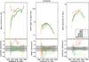 |
Fig. 1 Mode linewidth, mode height and mode amplitude (top), and relative values of these parameters with respect to the reference fit (bottom) as a function of mode frequency for various fitters for KIC 3733735. The grey band indicates the range of systematic error around the reference fit values of ±15% for mode linewidth and mode height, of ±5% for mode amplitude. The 1-σ error bars are those of Appourchaux. |
The model described above was used to fit the parameters of the 23 stars using maximum likelihood estimators (MLE) and with a Bayesian approach. For the MLE, formal uncertainties in each parameter were derived from the inverse of the Hessian matrix (for more details on MLE, significance, and formal errors, see Appourchaux 2011). For the Bayesian approach, the uncertainties (or credible intervals) were derived from the marginal posterior distribution of each parameter (for more details on credible intervals, see Benomar et al. 2009; Handberg & Campante 2011).
Tables 2 and A.1 provide a summary of the model used by each fitter team.
3.2. Guess parameter and fitting procedures
The procedure for the initial guess of the parameters is described in Appourchaux et al. (2012b), in which the steps of the fitting procedure are also described. These steps are repeated here for completeness:
-
1.
We fit the power spectrum as the sum of a stellar background made up of a combination of modified Lorentzian profiles (one or two) and white noise, as well as a Gaussian oscillation mode envelope with three parameters (the frequency of the maximum mode power, the maximum power, and the width of the mode power). Some fitters chose to exclude the p-mode region and fit the stellar background alone.
-
2.
We fit the power spectrum with n orders using the mode profile model described above, with no splitting and the stellar background fixed as determined in step 1.
-
3.
We follow step 2 but leave the rotational splitting and the stellar inclination angle as free parameters, and then apply a likelihood ratio test to assess the significance of the fitted splitting and inclination angle. For the Bayesian fit, step 2 is by-passed then step 3 is directly applied; this is because credible intervals are always provided for any parameter, hence the significance test is only applied by MLE fitters.
4. Sources of mode-linewidth and mode-height systematic errors, and their correction
When comparing the results that we obtained, it was clear that there are large differences in the mode linewidth and mode height measured by the different fitters. Figure 1 provides a typical example of large discrepancies between the fitters. The different sources of bias leading to the systematic errors observed are listed in Appendix A. The understanding of the different sources of bias provides a way to correct the systematic errors with respect to a reference fit. In short, the main sources of systematic error in the measurement of the mode linewidth and mode height are: 1) splitting bias and 2) stellar background bias. There are additional sources of systematic errors such as a different mode-height ratio and a different mean frequency which have been solved by assuming that the fitters use the same mode height ratio and mean frequency (see Appendix A for a full description of the various contributors).
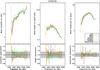 |
Fig. 2 Corrected mode linewidth, mode height, and mode amplitude (top), and relative values of these parameters with respect to the reference fit (bottom) as a function of mode frequency for KIC 3733735. The grey band indicates the range of systematic error around the reference fit values of ±15% for mode linewidth and mode height, of ±5% for mode amplitude. The error bars are those of the reference fit. |
In order to check that all of the sources of systematic errors encountered when comparing the different results can be understood and compensated for, we have implemented a correction scheme based upon the one-fit correction of Toutain et al. (2005). The procedure that they devised is based on fitting a spectrum model with no realisation noise (i.e. the limit spectrum) with a different spectrum model. The assumption behind that procedure is that the systematic errors are the same with the one-fit approach compared to a full Monte-Carlo simulation of the systematic errors resulting from using two different spectrum models. The correction scheme was applied for comparing with the results of the reference fit, which were provided by Appourchaux. The reference fit is simply used as a basis for understanding the source of the systematic errors. The reference fit value is in no way the best set but simply a data set that can provide a basis for understanding the impact of using a different fitting model due to different theoretical or observational constraints. The correction scheme is detailed in Appendix A.
The correction has been implemented for all fitters who provided the information on the stellar background, the splitting, and inclination angle, and compared to a reference fit. Figure 2 shows the correction results for the largest discrepancies already shown in Fig. 1. Figures B.1 to B.22 provide details of how the correction operates for all other stars on the mode linewidth and mode height. For 17 out of 23 stars, the correction scheme provides mode linewidths, mode heights, and mode amplitudes agreeing with the reference fit within ±15% for the first two parameters, and within ±5% for the last. As we showed above, the systematic error on the mode amplitude is bound to be smaller than for the mode linewidth or mode height alone. The correction is really effective especially when there are large discrepancies (Antia, Régulo) with respect to the reference fit for which the different stellar background is the major source, with in addition a different splitting in some cases. The remaining discrepancies (not larger than ±10%) mainly occur for the amplitude, especially when the mode height ratio used in the correction is far from the one used by the fitter. This is the case for KIC 1435467, KIC 3733735, KIC 3424541, and KIC 12258514 for some fitters (Benomar, Davies, Régulo) for which even the modified ratios of 1.0/2.0/1.0/0.0 were underestimating their fitted mode height ratio. Similar discrepancies (not larger than +30%) occur for mode linewidth when using a far-from-nominal mode height ratio for KIC 2837475 and KIC 7103006 (Régulo). In the latter case, the nominal mode height ratios of 1.0/1.5/0.5/0.05 overestimate the fitted mode height ratio. For the Antia results, there are also large discrepancies for 13 stars that are traced back to a mode height ratio varying largely from mode to mode and to the use of flat stellar background. In that case, neither a varying mode height ratio nor a flat stellar background are realistic assumptions regarding the fitting model.
Given the success encountered with the simple correction scheme, we chose not to make the correction model more detailed. Therefore, we assume that the reference fit values given in this paper are corrected for known systematic errors.
5. Results and discussion
Tables 3 to 25 provide the mode linewidth, mode height, and mode amplitude provided by the reference fit for all 23 stars of this study and the associated error bars. Figure 3 shows the dependence of the mode linewidth for the 23 stars of this study together with the l = 0 mode linewidths of 4 sub-giant stars of Benomar et al. (2013) and that of the Sun measured by the Luminosity Oscillations Imager (LOI) of VIRGO (Fröhlich et al. 1995; Appourchaux et al. 1997). We computed the mean power spectra of 16 years of full-disc time series of the LOI; the data were then analysed in a similar manner as for the 23 stars but using a dual modified Harvey profile for the background. For the data of Benomar et al. (2013), we divided the published amplitude by  because the values given in their paper were incorrectly quoted as
  (for a double-sided power spectrum), instead of
  (for a single-sided power spectrum as here); the mode height is unaffected by the correction since the former fit was performed on a single-sided spectrum. The figures are centred with respect to the frequency of the maximum of mode height. Figure 3 shows clearly that the linewidth dip disappears as the effective temperature increases. Figure 4 shows also that the maximum mode height and amplitude decrease with the effective temperature, as already shown by Kjeldsen & Bedding (1995). It is also interesting to note that the location of maximum mode height also corresponds to the location of the linewidth dip as anticipated by Belkacem et al. (2011), a location which does not coincide with the frequency of maximum amplitude, which is about half a large separation higher than the frequency of maximum mode height.
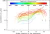 |
Fig. 3 Mode linewidth as a function of the mode order for the 23 stars with their colour identified by their effective temperature, for the l = 0 mode linewidths of 4 sub-giant stars of Benomar et al. (2013) (dashed lines), and for the solar LOI data (solid black line). For the 23 stars of this study the relative 1-σ error bars range from 5% to 10%, while those of Benomar et al. (2013) range from 10% to 20%. The 10% and 20% error bars are shown as an example. The longer LOI data set has relative error bars of about 2%. |
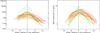 |
Fig. 4 Mode height and amplitude as a function of the mode order for the 23 stars with their colour identified by their effective temperature (as in Fig. 3), for the 4 sub-giant stars of Benomar et al. (2013) (dashed lines), and for the solar LOI data (solid black line). The relative 1-σ error bars for mode height are similar to those of the mode linewidth, while they are typically 3 times smaller for mode amplitude. |
In order to understand the dependence of the linewidth dip on effective temperature, we modelled the frequency dependence of the mode linewidth Γ as a combination of the power law dependence and the dip modelled as a Lorentzian profile in lnν: 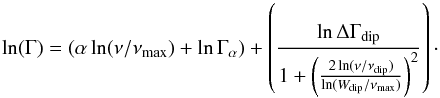 (1)where ν is the mode frequency, νmax is the frequency of maximum mode height, α is the power law index, Γα is the factor of the power law, ΔΓdip is the depth of the dip, Wdip is the width of the dip and νdip is the frequency of the dip. Figure 5 shows an example of a fitted linewidth using Eq. (1), clearly showing a dip. Figure 6 shows the result of the fit of the linewidth for all the stars of Fig. 3. The left-hand panels of Fig. 6 show the fit of the power-law only, for all 28 stars.
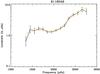 |
Fig. 5 Mode linewidth as a function of frequency for KIC 6116048 (solid line) with its 1-σ error bars compared with the fit following Eq. (1) (orange line). |
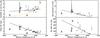 |
Fig. 6 Parameters of Eq. (1) as a function of the effective temperature for all 28 stars, for the power law dependence (left) and for the Lorentzian fit (right). The median value together with the credible intervals at 33% and 66% were derived from a Monte-Carlo simulation of the fit. The orange line shows the temperature dependence of the linewidth at the frequency of maximum mode height as derived by Appourchaux et al. (2012a). The open diamond is the result of the fit for the solar data of the LOI. The open triangles are the results of the fit for the sub-giant stars of Benomar et al. (2013). The solid lines show a linear fit of the parameters with respect to the effective temperature. The Lorentzian parameters for stars for which the Lorentzian fit is not significant are not plotted. |
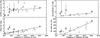 |
Fig. 7 Parameters of Eq. (1) as a function of the frequency of maximum mode height for all 28 stars, for the power law dependence (left) and for the Lorentzian fit (right). The median value together with the credible intervals of 33% and 66% were derived from a Monte-Carlo simulation of the fit. The open diamond is the result of the fit for the solar LOI data. The open triangles are the result of the fit for the sub-giant stars of Benomar et al. (2013). The error bars are derived from a Monte-Carlo simulation using credible intervals of 33% and 66%. The solid lines show a linear fit of the parameters with respect to the frequency. The Lorentzian parameters for stars for which the Lorentzian fit is not significant are not plotted. |
We checked whether the additional parameters of the Lorentzian profile of Eq. (1) were significant by examining the decrease in the reduced χ2 with respect to a χ2 law with 3 degrees of freedom; the probability cut was  ensuring that on average only one fit would be due to noise. In total there were 11 out of the 23 stars for which the 5-parameter fit was significant. In order to check the Gaussianity of the probability distribution of the parameters, we used Monte-Carlo simulations of the fit for returning the median value and its associated credible intervals. The non-Gaussianity of the distribution occurs only for two stars but the Monte-Carlo scheme is applied to all stars for coherence. The right-hand panels of Fig. 6 show the Lorentzian fit of the dip for 15 stars for which the dip was significant.
Linewidth parameters as per Eq. (1).
Figure 7 shows the result of the fit as a function of the frequency of maximum power, νmax, which is proportional to  , where g is the surface gravity and Teff is the effective temperature.
Chaplin et al. (1997) found that the solar mode linewidth follows a power law of 7 ± 1.5, at frequencies below 1800 μHz in agreement with the theoretical result of Balmforth (1992) and Goldreich & Murray (1994). Komm et al. (2000) found a power law index of about 3.3 for mode frequency excluding the linewidth dip extending from 2400 μHz to 3750 μHz for the Sun. In our case, the solar power law index is closer to that of Komm et al. (2000) because we made a global fit over a larger frequency range than that of the fit performed by Chaplin et al. (1997).
The width of the solar dip as measured by Komm et al. (2000) is about 1350 μHz wide (full width) which is about twice as large as the full width at half maximum that we found for the Sun. The right-hand panels of Fig. 6 clearly shows that the amplitude and the width of the dip decrease with the effective temperature. On the left top panel of Fig. 6, the dip also manifests itself as a deviation with respect to the linewidth measured at the maximum mode height (the orange line); the deviation becomes very small at high effective temperature.
It was shown by Komm et al. (2000) that the solar linewidth dip is reduced for increasing solar activity. The reduction was suggested to be due to the fact that radiative processes occurring in the upper superadiabatic boundary layer of the convection zone that are locally destabilizing, would be in turn less unstable because of an increasing magnetic field (Komm et al. 2000). But for other stars what is the source of the vanishing linewidth dip? Using data from a high-resolution spectrograph, Karoff et al. (2013) measured the flux of the chromospheric lines Ca II H&K of 11 stars in our study having a level of activity similar to that of the Sun. All of these stars fall in the category IV (low activity stars) of Vaughan & Preston (1980). KIC 3733735 and KIC 8379927 show a very high level of activity compared to the others of Karoff et al. (2013). KIC 3733735 has the highest effective temperature of our sample, and shows a dip that is at the limit of detection with very large error bars (see Figs. 2 and 6). On the other hand KIC 8379927 shows a measurable dip that might imply that this star is at minimum activity (see Fig. B.9). Therefore the reason for the absence of a dip in some active stars could be due to the stars being at their maximum activity. This can only be confirmed by measuring the activity of these stars over longer period of time.
Balmforth (1992) showed that the linewidth dip would disappear with an increasing mixing length parameter (α). Numerical simulations performed by Ludwig et al. (1999), Freytag & Salaris (1999) and Trampedach & Stein (2011) showed that the mixing length parameter decreases with effective temperature, and therefore a smaller mixing length parameter at high effective temperature would increase the depth of the linewidth dip contrary to what is observed in Fig. 6. Results based on stellar modelling by Pinheiro & Fernandes (2013) show an opposite dependence to that of the numerical simulations, e.g. the mixing length parameter increases with the effective temperature, being thus consistent with the findings of Fig. 6.
Houdek (1996) showed that the linewidth dip becomes more pronounced with decreasing surface density if the mixing-length parameter and anisotropy of the turbulent velocity field are kept constant in the model computations. For the stars studied in this paper, the surface density variations are dominated by changes in the effective temperature, i.e. the surface density decreases with increasing effective temperature provided the surface gravity stays approximately constant. For that case the linewidth dip would increase with increasing surface temperature, according to Houdek (1996), which is the opposite to what we found in Fig. 6. However, the properties of the linewidth dip also depend crucially on the anisotropy of the turbulent velocity field which calibration may lead to better agreements between model computations and observations.
These contradictory findings may have important impact for the modelling of convection and turbulence in stars.
6. Conclusions
We have analysed the oscillation power spectra of 23 main-sequence stars for which we obtained the mode linewidths, mode heights, and mode amplitude parameters. The parameters were obtained by a team of 8 independent fitters. We found large systematic errors between the parameters that could be traced to the way that the stellar background of the power spectrum was modelled; and to the fitted values of the rotational splitting and the stellar inclination angle. Other sources of systematic errors related to the mean frequency definition and to the mode height ratio were also studied. Finally using a correction scheme derived from the one-fit approach of Toutain et al. (2005), we could explain all sources of systematic errors, which could be reduced to less than ±15% for mode linewidth and mode height, and to less than ±5% for amplitude, when compared to a reference fit value. A different stellar background will give rise to frequency-dependent systematic errors that might affect the comparison with theoretical mode linewidth and mode height, therefore affecting the understanding of the physical nature of these parameters. All other sources of relative systematic errors are independent of frequency.
Using the 23 stars of this study, 4 additional sub-giant stars of Benomar et al. (2013) and solar data, we also derived that the amplitude of the linewidth dip close to the maximum of frequency decreases with effective temperature. The dependence of the dip with effective temperature is linked to the behaviour of convection in the stellar atmosphere, implying that either the mixing length or the level of activity may increase with effective temperature.
Online material
Mode heights, mode linewidths and mode amplitude for KIC 1435467.
Mode heights, mode linewidths and mode amplitude for KIC 2837475.
Mode heights, mode linewidths and mode amplitude for KIC 3424541.
Mode heights, mode linewidths and mode amplitude for KIC 3733735.
Mode heights, mode linewidths and mode amplitude for KIC 6116048.
Mode heights, mode linewidths and mode amplitude for KIC 6508366.
Mode heights, mode linewidths and mode amplitude for KIC 6679371.
Mode heights, mode linewidths and mode amplitude for KIC 7103006.
Mode heights, mode linewidths and mode amplitude for KIC 7206837.
Mode heights, mode linewidths and mode amplitude for KIC 8379927.
Mode heights, mode linewidths and mode amplitude for KIC 8694723.
Mode heights, mode linewidths and mode amplitude for KIC 9139151.
Mode heights, mode linewidths and mode amplitude for KIC 9139163.
Mode heights, mode linewidths and mode amplitude for KIC 9206432.
Mode heights, mode linewidths and mode amplitude for KIC 9812850.
Mode heights, mode linewidths and mode amplitude for KIC 10162436.
Mode heights, mode linewidths and mode amplitude for KIC 10162436.
Mode heights, mode linewidths and mode amplitude for KIC 10355856.
Mode heights, mode linewidths and mode amplitude for KIC 10454113.
Mode heights, mode linewidths and mode amplitude for KIC 10909629.
Mode linewidths, mode heights and mode amplitude for KIC 11081729.
Mode linewidths, mode heights and mode amplitude for KIC 12009504.
Mode linewidths, mode heights and mode amplitude for KIC 12258514
Mode linewidths, mode heights and mode amplitude for KIC 12317678.
Appendix A: Source of systematic errors and their correction
In this appendix, we mainly focus on internal differences resulting from different fit assumptions, which led to different fitted results. The observation duration, being common to all fitters, was excluded from the possible source of systematic errors; in addition since the observation duration was larger than 30 times the longest mode lifetime (see Chaplin et al. 2008) this source of external systematic error was negligible. We also note, that the values of mode linewidths, and mode heights obtained with MLE are derived from the mean value of the natural logarithm of these parameters, while the Bayesian values are obtained from the median of these parameters (Benomar et al. 2009), resulting in differences between the two statistical values of less than a few percent, thanks to the long observation duration.
The large deviations between the results obtained leads to an investigation of the possible sources of systematic errors, which are:
-
Bias on the estimated stellar background.
-
Bias on the estimated splitting and inclination angle.
-
Bias on the assumed mode height ratio.
-
Different definition of the mean frequency.
Hereafter we detail each source of systematic error from a theoretical and practical point of view. The theoretical understanding of the systematic errors is based on the use of MLE for mode extraction. Other extracting methods used in this paper derive the mode parameters in a Bayesian framework (Benomar et al. 2009; Handberg & Campante 2011). The two methods are obviously not identical since the Bayesian approach used a priori information on the parameters to be fitted which will slant the outcome in a different manner. We deliberately chose not to take account of these additional systematic errors, which are far more difficult to model than those resulting from using the MLE approach. The correction approach based upon an MLE fit proved its efficacy, showing that there was no need to take into account the Bayesian parameter derivation in the correction scheme.
Table A.1 lists the model characteristics of each fitter whose differences lead to systematic errors in the mode linewidth and height.
Model parameters affecting directly the stellar background, mode linewidth, and mode height.
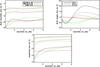 |
Fig. A.1 Mode parameter biases as a function of linewidth for a stellar background bias of +1%, for several signal-to-noise ratios and for three different kinds of profiles which are: a triplet l = 0,1,2,3 with a splitting of 2 μHz with the mode pairs l = 0 − 2 and l = 1 − 3 separated by 120 μHz (black line); a triplet with a splitting of 6 μHz with the mode pair l = 0 − 2 and l = 1 − 3 separated by 120 μHz (green line); and a single mode profile (red line). (Top, left) For mode linewidth, (top, right) For mode height ratio, (bottom, left) For mode amplitude. |
Appendix A.1: Effect of an incorrect estimation of the stellar background
One might naively assume that an underestimated stellar background would lead to an overestimated mode height compensating the reduced stellar background. This naive approach would provide an underestimated linewidth. Fortunately, the effect of an incorrect estimation of the stellar background on the mode can be analytically calculated which provides a counter intuitive result. The relations between the mode-linewidth, mode-height and mode-amplitude systematic errors which lead to an incorrect estimated stellar background are given in Appendix B.2. In short, an underestimation of the stellar background will lead to an underestimation of the mode height and an overestimation of the linewidth. In addition, the lower the signal-to-noise ratio the higher the systematic error on mode linewidth and height (the signal-to-noise ratio is the ratio of mode height to the stellar background). The systematic errors were also numerically derived using the technique of the fit of a single (not many) profile of Toutain et al. (2005), i.e. by simulation of the MLE for a single profile fitted by a profile with a different stellar background. Figure A.1 shows the results of the numerical calculation of the mode linewidth, mode height, and mode amplitudes biases as a function of mode linewidth, for several signal-to-noise ratio. Assuming that the background is overestimated by 1%, then when the signal-to-noise ratio is about 10, the mode linewidth is typically underestimated by about 1.75%, while the mode height is overestimated by about 0.75 %. The sign of the mode-linewidth systematic error is opposite to that of the mode-height systematic error, such that they almost compensate each other when computing the mode-amplitude systematic errors. It means that an overestimation of the stellar background of 1% will provide a mode amplitude underestimated by 0.5%.
When the signal-to-noise ratio is close to 1, the mode-linewidth systematic errors increases to about −8% while the mode-height systematic errors are only 2%. This is what was observed in some stars for which we could not understand why the systematic error on the linewidth was so much larger than for the mode height. As a consequence, care should be taken when comparing amplitudes of different fitters when the signal-to-noise ratio is low.
We also note that when the signal-to-noise ratio increases, the mode-amplitude systematic error gets smaller and smaller, i.e. a 1% stellar background overestimation would provide a 0.1% mode amplitude underestimation. This explains why the mode amplitude differences between different fits may be very small but not necessarily absent when the signal-to-noise ratio is high.
The differences between the different fitted stellar backgrounds can vary between 30% in the worst case to about 10% in the best cases. The differences are mainly due to the model of the stellar background used having one or several components as shown in Table A.1. It must be pointed out that since the background bias varies with frequency, this will also introduce a varying effect on the relative variation of the mode linewidth and mode height.
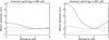 |
Fig. A.2 Relative systematic error of three parameters of the l = 0 − 2 and l = 1 − 3 modes as a function of the fitted splitting: mode linewidth (solid line), mode height (dotted line), mode amplitude (dashed line) for a signal-to-noise ratio of 1, a nominal splitting of 4 μHz and an inclination angle of 90 degrees. Left: the multiplet has a nominal linewidth of 6 μHz. Right: the multiplet has a nominal linewidth of 3 μHz. |
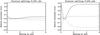 |
Fig. A.3 Relative systematic error of three parameters of the l = 0 − 2 and l = 1 − 3 modes as a function of the fitted splitting: mode linewidth (solid line), mode height (dotted line), mode amplitude (dashed line) for a signal-to-noise ratio of 1, a nominal splitting of 0.4 μHz and an inclination angle of 90 degrees. Left: the multiplet has a nominal linewidth of 3 μHz. Right: the multiplet has a nominal linewidth of 1 μHz. |
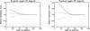 |
Fig. A.4 Relative systematic error on three parameters of the l = 0 − 2 and l = 1 − 3 multiplet as function of the fitted inclination angle: mode linewidth (solid line), mode height (dotted line), mode amplitude (dashed line) for a signal-to-noise ratio of 1. The multiplet has a nominal linewidth of 6 μHz and a nominal splitting of 4 μHz, with a nominal inclination angle of 45 degrees (left), and a nominal inclination angle of 90 degrees (right). |
Appendix A.2: Effect of a different estimated splitting and inclination angle
The effect of a different estimated splitting can also be simply understood when, for example, a null splitting is fitted when the modes are genuinely split: this will lead to an overestimation of the linewidth. The analytical calculations of the effect are detailed in Appendix B.3 but do not lead to simple useful formula; the only result being that second order effects dominate. This is the reason why we simulated an l = 0 − 2 pair and an l = 1 − 3 pair with a symmetrical rotational splitting and with mode height ratio of 1/1.5/0.5/0.05 for the l = 0,1,2,3, respectively. We then applied the one-fit method of Toutain et al. (2005) for computing the systematic errors. Figures A.2 to A.4 show results for three different cases.
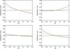 |
Fig. A.5 Relative systematic error as a function of the deviation to the reference mode visibility for the mode height (black line) and linewidth (orange line) for a set of l = 0,1,2 modes with a 2-μHz linewidth, and a signal-to-noise ratio 10 for the l = 0 mode. The continuous lines are the systematic error computed using the method of Toutain et al. (2005). The dashed line is the analytical systematic error on mode height derived assuming there is no systematic error on the linewidth derived from Eq. (B.38). Top left: the deviations to the reference mode visibilities are identical for l = 1 and l = 2. Bottom left: the deviations to the reference mode visibilities are of opposite sign for l = 1 and l = 2. Top right: the deviation to the reference mode visibilities is zero for l = 2. Bottom right: the deviation to the reference mode visibilities is zero for l = 1. |
In Fig. A.2, for a 90-degree inclination (perpendicular to the line of sight), when the nominal splitting is of the order of the linewidth, the fitted linewidth with a null fitted splitting will be typically overestimated by the value in excess of a few times the nominal splitting. In Fig. A.3, for a 90-degree inclination (perpendicular to the line of sight), when the nominal splitting is about 10% to 20% of the linewidth, the fitted linewidth with a null fitted splitting will be typically overestimated by the value smaller than the nominal splitting. We also note that the dependence of the linewidth bias on to the splitting is quadratic close to the nominal splitting but not exactly at the nominal splitting. At the local minimum, the systematic error is slightly negative, although the systematic error at the nominal splitting is null.
In Fig. A.4, we also simulated a varying inclination, assuming that the projected splitting was kept constant ( ). The reason for using such a formulation is that the fit preferentially converges towards a value for which
  is constant as shown by Ballot et al. (2006). The systematic errors remain small when the fitted inclination angle is greater than 45 degrees. In addition the systematic errors decrease with the inclination angle. Therefore a correction is clearly necessary when the fitted inclination angles are less than 45 degrees while the fitted reference inclination angle is above 45 degrees, i.e. a difference of about 45 degrees will produce large systematic errors in the mode parameters.
If one assumes the same splitting and inclination angle for all modes, the splitting and angle systematic errors introduce a frequency dependence on the relative variation of the mode linewidth and mode height when compared to the reference fit values. The frequency dependences on the relative errors are larger at smaller linewidths, emphasising the need for a proper estimation of the splitting at the low-frequency part of the spectrum.
Appendix A.3: Effect of different assumptions on mode height ratio
Some fitters also allow the mode height ratio to vary, which will also lead, when compared to the results obtained with a notional mode height ratio, to some systematic error in the measured linewidth and mode height. Neglecting the systematic error on mode linewidth, we analytically computed the systematic error on mode height (see Appendix B.4). We also applied the one-fit method of Toutain et al. (2005) for computing the systematic errors. Figure A.5 shows the results of the analytical and numerical calculations of the systematic errors on mode linewidth, mode height, and mode amplitudes biases as a function of deviations to the reference mode height ratio for a set of l = 0,1,2 modes with a 2-μHz linewidth, and a signal-to-noise ratio of 10 for the l = 0 mode.
To first order, the impact of a different mode height ratio on the linewidth is rather small and typically of the order of 10%. On the other hand, the impact of a different mode height ratio is much larger on the mode height, being close to 40% in the worst case. In addition, the systematic error on the mode height ratio will produce a non-negligible systematic error on the mode amplitude. Ballot et al. (2011) showed, using adiabatic computations, that the mode height ratio varies with the effective temperature, surface gravity, and metallicity. For the stars listed in this study, using the work of Ballot et al. (2011) and the stellar parameters provided by Bruntt et al. (2012) we derived that the mode height ratio for l = 1, l = 2, l = 3 is 1.5, 0.52, 0.025 varying by 0.02, 0.02, 0.004, respectively.
As shown by Salabert et al. (2011) for the solar case, the measured ratios agree very well with the theoretical ratios to within 0.06 and do not vary with time. Such a deviation of 0.06 would result in systematic errors not larger than 4% for the mode height, a value that can also be derived from Eq. (B.38). The values derived above from Ballot et al. (2011) would provide even a smaller systematic error not larger than 2%. Larger deviations of stellar mode ratio with respect to the value given above were also observed (Salabert 2013, priv. comm.). At the time of writing, given that the variation of the mode height ratio is primarily geometrical, there is very little variation with mode frequency. Then, in order to achieve a repeatable measurement, it is advised to keep the mode height ratio at reference values of 1.5, 0.5, 0.05 for l = 1, l = 2, and l = 3, respectively.
 |
Fig. A.6 Relative systematic error as a function of frequency for a mean frequency shifted by half the large separation for the solar case for mode linewidth (left) and for mode height (right) using BiSON data (black line, Chaplin et al. 1997) and GONG data (orange line, Komm et al. 2000). |
Appendix A.4: Effect of a different definition of mean frequency
By definition of the model, the linewidth is set to be common for modes that are within half a large separation. There are two possible configurations defining for which modes the linewidth will be common: configuration A for which the l = 0,2 mode pair is at the left of the l = 1 mode; and configuration B for which the l = 0,2 mode pair is at the right of the l = 1 mode. As a result, the mean frequency will differ for the different configurations. For configuration A, the mean frequency is νn,0 + Δν/ 4, while for configuration B, it is νn,0 − Δν/ 4. Therefore depending on how the fits are performed there could be up to a Δν/ 2 difference in the mean frequency. Since it is assumed that the mode linewidth only depends upon mode frequency, this would directly produce a systematic error that would be proportional to the linewidth frequency derivative and the frequency difference.
Figure A.6 shows the resulting relative systematic error on mode linewidth and mode height in the solar case using BiSON and GONG data. The relative error could be up to 40% especially at the low frequencies. Fortunately, the signal-to-noise ratio of the Kepler observations allows the observation of low order modes only for stars more massive than the Sun having higher mode amplitude. These stars then have smaller large separation than the Sun, typically about the third of the solar case. Therefore the relative error due to the different mean frequency is never larger than 10% for either the mode linewidth or the mode height.
Finally, only one fitter (Howe) used the formal order definition for which the l = 2 mode is separated by a large separation of the l = 0 mode of the same order n (configuration a in Table A.1). The problem of using this formal definition for fitting across a large separation is that the l = 2 mode of order n is very close to the l = 0 mode of order n + 1. In practice, then the formal order definition is almost never used for mode fitting. In any case, the difference of mean frequency of configuration A with respect to the formal order definition is then only Δν/ 4. It means that the systematics, resulting from the different definition in that case, are twice as small as those resulting from using configuration B, or less than 5%.
Appendix A.5: Implementation of the correction of the systematic errors
For each fit, the correction was computed by modelling the l = 0 − 2 and l = 1 − 3 modes over a window as large as the large separation (Δν) with the pair of modes separated by half of that. The large separation is 240 μHz. The l = 2 and l = 3 modes are assumed to be 6 μHz and 10 μHz to the left of their adjacent l = 0 or l = 1 mode. The correction could have been implemented with the proper large separation for each star but the results shows that the correction works even with the default large separation we used. The mode height ratios are assumed to be either 1.0/1.5/0.5/0.05 or 1.0/2.0/1.0/0.0, depending on the star or the fitter. The latter mode height ratio were typical results obtained by some fitters when freeing the ratios. The linewidth is common to the set of mode frequencies following configuration A. We note that the differences in the mean frequency between the different configurations were not implemented in the correction because of the rather small biases introduced. The stellar background is flat. The profile is modelled using the reference fit with the measured linewidth, mode height, splitting, inclination angle and stellar background. Since the value of the background is taken at the l = 0 mode, we neglect the frequency dependence of the stellar background within a large separation. In the worst case the differential variation of the fitted stellar background with respect to the reference fit is typically less than 0.5% across a large separation which is negligible compared to other systematic errors. The fit is performed for only the linewidth and mode height as free parameters with a fixed splitting, inclination angle, and stellar background provided by each fitter using the one-fit approach of Toutain et al. (2005). Finally, the correction of the systematic errors is computed by taking the ratio of the fitted linewidth or mode height to that of the reference fit.
We emphasize that the correction scheme could have been improved by using the mode-frequency configuration of each fitter, the true fitted mode height ratio of each mode or of the ensemble of modes and a non-flat stellar background. The simple correction scheme is sufficiently efficient to argue against making the correction model more complex.
Figures B.1 to B.22 show for the remaining 22 stars the mode linewidth, height, and amplitude corrected for systematic errors using the procedure described above.
Appendix B: Analytical derivation of the biases leading to systematic errors
Appendix B.1: Assumptions
The mode parameters are usually extracted from the power spectra using MLE which consists in finding the maximum of the following figure of merit (See Toutain & Appourchaux 1994, for details):  (B.1)where S1 is the model of the power spectra, S(νk) represents the spectral data at the frequency bin νk, λ is the vector of parameters (frequency, splitting, linewidth, etc.). In order to find the maximum of Eq. (B.1), one needs to compute the derivative with respect to λ. At the maximum, the derivative should be zero for all values of the element of the vector λ:
 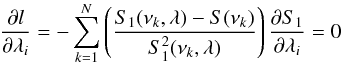 (B.2)which can be approximated, as per Toutain & Appourchaux (1994), by:
 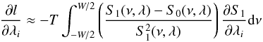 (B.3)where ν is the frequency, W is the frequency range over which the maximization is performed, T is the observation duration and S0 is the asymptotic mean spectra.
The procedure used for analytically finding the systematic errors is then simply to use the fact that  for all λi. The analytical derivation can then be compared with the one-fit approach of Toutain et al. (2005), which explicitly assumes that the bias obtained by fitting an observed spectrum S(ν) with a profile S1(ν,λ) is the same as fitting the asymptotic noiseless profile S0(ν,λ). The procedure used by Toutain et al. (2005) is then simply to fit S0(ν,λ) once instead of doing Monte-Carlo simulations of many realisation of S(ν). With this procedure, this is exactly the asymptotic expression of Eq. (B.1) that one maximises, which results in finding asymptotically the zero of
  as a function of the parameters λi.
In all of the following subsections, we assumed a symmetrical Lorentzian profile for the asymptotic and fitted profiles.
Appendix B.2: Effect of an incorrect estimation of the stellar background
When the fitted spectra S1 is different from S0, we can write to first order: 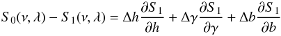 (B.4)where γ = lnΓ, h = lnH, b = lnB with Γ, H, and B being the mode linewidth, the mode height and the stellar background, respectively. We note that if we assume that the model of the mode profile includes a white noise background, we have
  . Inserting Eqs. (B.4) in (B.3), one gets for the derivative with respect to γ and h:
 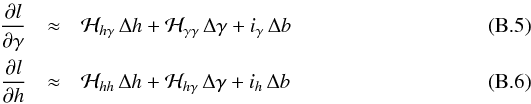 where ℋhγ, ℋγγ and ℋhh are the elements of the Hessian ℋ given by Toutain & Appourchaux (1994) as:
 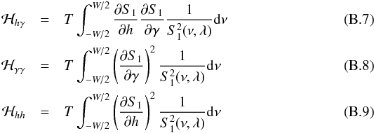 and with:
 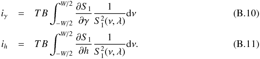 Since
Since  by construction of the MLE solution, Eqs. (B.5) and (B.6) will provide the solution for Δh and Δγ as a function of Δb as:
 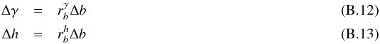 with
with 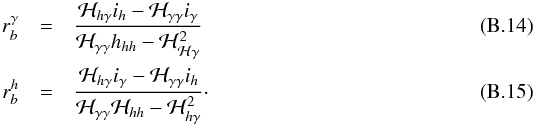 The bias on the mode amplitude can be expressed as
 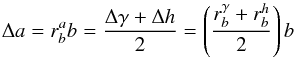 (B.16)where a = lnA. Equations (B.12) and (B.13) are the ratios for a notional bias in B. Since the calculation provided above was done assuming that the frequency window was large with respect to the mode linewidth, we must point out that the stellar background itself may be substantially over- or underestimated when the linewidth is not small compared to the window of interest. As a consequence, even though the sensitivity to the background bias may be small, it is likely that the effective biases on mode linewidth and mode height may be larger because the bias on the stellar background may be large.
Appendix B.3: Effect of a different estimated splitting and inclination angle
As shown by Toutain & Appourchaux (1994), there is no correlation between the splitting error and the mode linewidth error or the mode height error. It implicitly means that at least to first order there should not be any systematic errors in the mode linewidth and mode height measurements resulting from an incorrectly estimated splitting. We study here is the second order effect.
When the fitted spectra S1 is different from S0, we can write to the second order : ![Mathematical equation: \appendix \setcounter{section}{2} \begin{eqnarray} S_{0}(\nu,\lambda)-S_{1}(\nu,\lambda)&=&\sum_j \Delta \lambda_j \frac{{\partial} S_{1}}{\partial {\lambda_j}}+\sum_{j \ne k} \Delta \lambda_j \Delta \lambda_k \frac{{\partial} S_{1}}{\partial {\lambda_j}}\frac{{\partial} S_{1}}{\partial {\lambda_k}}\nonumber\\[2mm] &&+\,\sum_{j} \frac{\Delta \lambda_j^2}{2}\frac{{\partial}^2 S_{1}}{\partial {\lambda_j^2}} \label{b17} \end{eqnarray}](/articles/aa/full_html/2014/06/aa23317-13/aa23317-13-eq107.png) (B.17)where λj are γ,h, b and νs (where νs is the mode splitting of the multiplet). Inserting Eqs. (B.17) in (B.3) one gets:
(B.17)where λj are γ,h, b and νs (where νs is the mode splitting of the multiplet). Inserting Eqs. (B.17) in (B.3) one gets: ![Mathematical equation: \appendix \setcounter{section}{2} \begin{eqnarray} \frac{{\partial} l}{\partial {\lambda_i}} &\approx & T \int_{-W/2}^{W/2} \left[\sum_j \Delta \lambda_j \frac{{\partial} S_{1}}{\partial {\lambda_j}}+\sum_{j \ne k} \Delta \lambda_j \Delta \lambda_k \frac{{\partial} S_{1}}{\partial {\lambda_j}}\frac{{\partial} S_{1}}{\partial {\lambda_k}}\right] \frac{{\partial} S_{1}}{\partial {\lambda_i}} {\rm d}\nu \nonumber\\[2mm] &&+\,T \int_{W/2}^{W/2}\left[\sum_{j} \frac{\Delta \lambda_j^2}{2}\frac{{\partial}^2 S_{1}}{\partial {\lambda_j^2}}\right] \frac{{\partial} S_{1}}{\partial {\lambda_i}} {\rm d}\nu. \label{b18} \end{eqnarray}](/articles/aa/full_html/2014/06/aa23317-13/aa23317-13-eq112.png) (B.18)Here we note that the parity with respect to frequency (ν) will play a key role in whether some terms disappears or not. For instance, all derivatives of S1 with respect to γ, h and b will be even in (ν − ν0), where ν0 is the central mode frequency of the multiplet. The derivatives of S1 with respect to ν0 are odd in (ν − ν0) while the derivative of S1 with respect to νs is even in (ν − ν0). Therefore of all the cross terms involving γ,h,b, and ν0 are null. At first sight all of the cross terms with νs would not necessarily be null. But since the multiplet is composed of a superposition of several peaks, there is a local parity in the function around the mode frequency νlm, i.e. around (ν − νlm) which Toutain & Appourchaux (1994) termed as locally odd (or even) function, in other words:
(B.18)Here we note that the parity with respect to frequency (ν) will play a key role in whether some terms disappears or not. For instance, all derivatives of S1 with respect to γ, h and b will be even in (ν − ν0), where ν0 is the central mode frequency of the multiplet. The derivatives of S1 with respect to ν0 are odd in (ν − ν0) while the derivative of S1 with respect to νs is even in (ν − ν0). Therefore of all the cross terms involving γ,h,b, and ν0 are null. At first sight all of the cross terms with νs would not necessarily be null. But since the multiplet is composed of a superposition of several peaks, there is a local parity in the function around the mode frequency νlm, i.e. around (ν − νlm) which Toutain & Appourchaux (1994) termed as locally odd (or even) function, in other words: 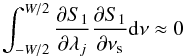 (B.19)with λj ≠ νs. We can then rewrite Eq. (B.18) for the splitting νs as
 ![Mathematical equation: \appendix \setcounter{section}{2} \begin{equation} \frac{{\partial} l}{\partial {\nu_{\rm s}}} \approx \left[\Delta \nu_{\rm s} {\cal H}_{\nu_{\rm s} \nu_{\rm s}}\right]+\left(\sum_{j \ne k}\Delta \lambda_j \Delta \lambda_k g_{jk}^{\nu_{\rm s}} + \sum_{j} \frac{\Delta \lambda_j^2}{2} g_{jj}^{\nu_{\rm s}}\right) \label{b20} \end{equation}](/articles/aa/full_html/2014/06/aa23317-13/aa23317-13-eq120.png) (B.20)\pagebreak
(B.20)\pagebreak
and then for γ,h and b (=λi′) as: ![Mathematical equation: \appendix \setcounter{section}{2} \begin{equation} \frac{{\partial} l}{\partial \lambda_{i'}} \approx \left[\sum_{\lambda_j \ne \nu_{\rm s}} \Delta \lambda_{j} {\cal H}_{ji'}\right]+\left(\sum_{j \ne k}\Delta \lambda_j \Delta \lambda_k g_{jk}^{i'} + \sum_{j} \frac{\Delta \lambda_j^2}{2} g_{jj}^{i'}\right) \label{b21} \end{equation}](/articles/aa/full_html/2014/06/aa23317-13/aa23317-13-eq122.png) (B.21)where
(B.21)where  is written as:
 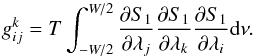 (B.22)The terms in brackets in Eqs. (B.20) and (B.21) represent the first order terms, while the terms in parentheses are the higher order terms. Since by construction of the MLE solution, it is clear that the solution to the system of equation is non-linear. As a consequence, the systematic errors on mode linewidth and mode height strongly depend to the second order to deviation to the nominal splitting.
This simple analysis shows that the derivation of the biases due to splitting is not straightforward. This is why we resorted to the single-fit approach of Toutain et al. (2005) in order to have some clues as to the magnitude of the effect of an incorrect splitting. Figures A.2 and A.3 shows the results of the numerical calculation of the systematic errors on mode linewidth, mode height, and mode amplitude biases as a function of the fitted splitting, for two different nominal splitting and mode linewidth. Figure A.4 shows the results of the numerical calculation of the systematic errors on mode linewidth, mode height, and mode amplitude biases as a function of the fitted inclination angle, for a single nominal splitting and mode linewidth, and for two nominal inclination angles.
Appendix B.4: Effect of different assumption on mode height ratio
Here we assume that the fitted mode profile is given by a superposition of a profile for each l such that we can write  (B.23)where
  is the fixed (or fitted) mode height ratio normalised to the l = 0 degree, i.e.
  . We have a similar expression for the reference profile S0 introducing the mode height H and the mode height ratio αl. Therefore we can write that:
 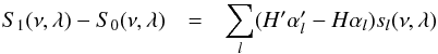 (B.24)Using Eq. (B.3) we can write for the fitted mode height:
 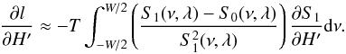 (B.25)Deriving Eq. (B.23) with respect to H′, we have:
 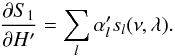 (B.26)Since
  , using Eqs. (B.24), (B.25) and (B.26) we can derive that we have:
  (B.27)\newpagewith
 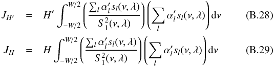 assuming that the cross terms between different l are negligible, Eqs. (B.28) and (B.29) can be approximated as:
 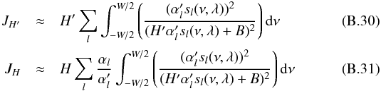 both equations can be simplified as
 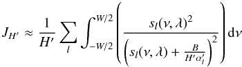 (B.32)and
 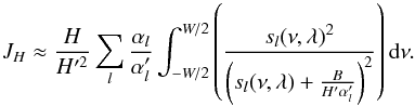 (B.33)We can calculate these integrals using Eq. (A1) of Toutain & Appourchaux (1994) by replacing β by β′/α′, where β′ = B/H′ and assuming that the frequency window is large compared to the linewidth. Omitting the common factors, we finally obtain:
 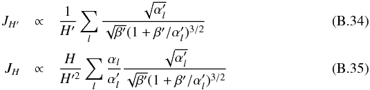 then using Eq. (B.27), we have:
  (B.36)Then to first order in ΔH = H′ − H and in
  , we can write
  (B.37)such that we have the following approximation:
  (B.38)
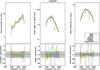 |
Fig. B.1 Corrected mode linewidth, mode height, and mode amplitude (top), and relative values of these parameters with respect to the reference fit (bottom) as a function of mode frequency for KIC 1435467. The grey band indicates the range of systematic error around the reference fit values of ±15% for mode linewidth and mode height, of ±5% for mode amplitude. The error bars are those of the reference fit. |
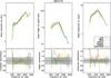 |
Fig. B.2 Corrected mode linewidth, mode height, and mode amplitude (top), and relative values of these parameters with respect to the reference fit (bottom) as a function of mode frequency for KIC 2837475. The grey band indicates the range of systematic error around the reference fit values of ±15% for mode linewidth and mode height, of ±5% for mode amplitude. The error bars are those of the reference fit. |
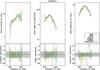 |
Fig. B.3 Corrected mode linewidth, mode height, and mode amplitude (top), and relative values of these parameters with respect to the reference fit (bottom) as a function of mode frequency for KIC 3424541. The grey band indicates the range of systematic error around the reference fit values of ±15% for mode linewidth and mode height, of ±5% for mode amplitude. The error bars are those of the reference fit. |
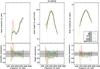 |
Fig. B.4 Corrected mode linewidth, mode height, and mode amplitude (top), and relative values of these parameters with respect to the reference fit (bottom) as a function of mode frequency for KIC 6116048. The grey band indicates the range of systematic error around the reference fit values of ±15% for mode linewidth and mode height, of ±5% for mode amplitude. The error bars are those of the reference fit. |
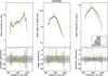 |
Fig. B.5 Corrected mode linewidth, mode height, and mode amplitude (top), and relative values of these parameters with respect to the reference fit (bottom) as a function of mode frequency for KIC 6508366. The grey band indicates the range of systematic error around the reference fit values of ±15% for mode linewidth and mode height, of ±5% for mode amplitude. The error bars are those of the reference fit. |
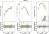 |
Fig. B.6 Corrected mode linewidth, mode height, and mode amplitude (top), and relative values of these parameters with respect to the reference fit (bottom) as a function of mode frequency for KIC 6679371. The grey band indicates the range of systematic error around the reference fit values of ±15% for mode linewidth and mode height, of ±5% for mode amplitude. The error bars are those of the reference fit. |
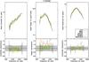 |
Fig. B.7 Corrected mode linewidth, mode height, and mode amplitude (top), and relative values of these parameters with respect to the reference fit (bottom) as a function of mode frequency for KIC 7103006. The grey band indicates the range of systematic error around the reference fit values of ±15% for mode linewidth and mode height, of ±5% for mode amplitude. The error bars are those of the reference fit. |
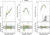 |
Fig. B.8 Corrected mode linewidth, mode height, and mode amplitude (top), and relative values of these parameters with respect to the reference fit (bottom) as a function of mode frequency for KIC 7206837. The grey band indicates the range of systematic error around the reference fit values of ±15% for mode linewidth and mode height, of ±5% for mode amplitude. The error bars are those of the reference fit. |
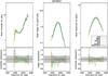 |
Fig. B.9 Corrected mode linewidth, mode height, and mode amplitude (top), and relative values of these parameters with respect to the reference fit (bottom) as a function of mode frequency for KIC 8379927. The grey band indicates the range of systematic error around the reference fit values of ±15% for mode linewidth and mode height, of ±5% for mode amplitude. The error bars are those of the reference fit. |
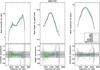 |
Fig. B.10 Corrected mode linewidth, mode height, and mode amplitude (top), and relative values of these parameters with respect to the reference fit (bottom) as a function of mode frequency for KIC 8694723. The grey band indicates the range of systematic error around the reference fit values of ±15% for mode linewidth and mode height, of ±5% for mode amplitude. The error bars are those of the reference fit. |
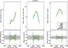 |
Fig. B.11 Corrected mode linewidth, mode height, and mode amplitude (top), and relative values of these parameters with respect to the reference fit (bottom) as a function of mode frequency for KIC 9139151. The grey band indicates the range of systematic error around the reference fit values of ±15% for mode linewidth and mode height, of ±5% for mode amplitude. The error bars are those of the reference fit. |
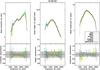 |
Fig. B.12 Corrected mode linewidth, mode height, and mode amplitude (top), and relative values of these parameters with respect to the reference fit (bottom) as a function of mode frequency for KIC 9139163. The grey band indicates the range of systematic error around the reference fit values of ±15% for mode linewidth and mode height, of ±5% for mode amplitude. The error bars are those of the reference fit. |
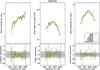 |
Fig. B.13 Corrected mode linewidth, mode height, and mode amplitude (top), and relative values of these parameters with respect to the reference fit (bottom) as a function of mode frequency for KIC 9206432. The grey band indicates the range of systematic error around the reference fit values of ±15% for mode linewidth and mode height, of ±5% for mode amplitude. The error bars are those of the reference fit. |
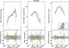 |
Fig. B.14 Corrected mode linewidth, mode height, and mode amplitude (top), and relative values of these parameters with respect to the reference fit (bottom) as a function of mode frequency for KIC 9812850. The grey band indicates the range of systematic error around the reference fit values of ±15% for mode linewidth and mode height, of ±5% for mode amplitude. The error bars are those of the reference fit. |
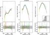 |
Fig. B.15 Corrected mode linewidth, mode height, and mode amplitude (top), and relative values of these parameters with respect to the reference fit (bottom) as a function of mode frequency for KIC 10162436. The grey band indicates the range of systematic error around the reference fit values of ±15% for mode linewidth and mode height, of ±5% for mode amplitude. The error bars are those of the reference fit. |
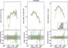 |
Fig. B.16 Corrected mode linewidth, mode height, and mode amplitude (top), and relative values of these parameters with respect to the reference fit (bottom) as a function of mode frequency for KIC 10355856. The grey band indicates the range of systematic error around the reference fit values of ±15% for mode linewidth and mode height, of ±5% for mode amplitude. The error bars are those of the reference fit. |
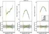 |
Fig. B.17 Corrected mode linewidth, mode height, and mode amplitude (top), and relative values of these parameters with respect to the reference fit (bottom) as a function of mode frequency for KIC 10454113. The grey band indicates the range of systematic error around the reference fit values of ±15% for mode linewidth and mode height, of ±5% for mode amplitude. The error bars are those of the reference fit. |
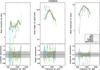 |
Fig. B.18 Corrected mode linewidth, mode height, and mode amplitude (top), and relative values of these parameters with respect to the reference fit (bottom) as a function of mode frequency for KIC 10909629. The grey band indicates the range of systematic error around the reference fit values of ±15% for mode linewidth and mode height, of ±5% for mode amplitude. The error bars are those of the reference fit. |
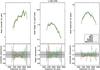 |
Fig. B.19 Corrected mode linewidth, mode height, and mode amplitude (top), and relative values of these parameters with respect to the reference fit (bottom) as a function of mode frequency for 11081729. The grey band indicates the range of systematic error around the reference fit values of ±15% for mode linewidth and mode height, of ±5% for mode amplitude. The error bars are those of the reference fit. |
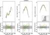 |
Fig. B.20 Corrected mode linewidth, mode height, and mode amplitude (top), and relative values of these parameters with respect to the reference fit (bottom) as a function of mode frequency for 12009504. The grey band indicates the range of systematic error around the reference fit values of ±15% for mode linewidth and mode height, of ±5% for mode amplitude. The error bars are those of the reference fit. |
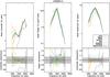 |
Fig. B.21 Corrected mode linewidth, mode height, and mode amplitude (top), and relative values of these parameters with respect to the reference fit (bottom) as a function of mode frequency for 12258514. The grey band indicates the range of systematic error around the reference fit values of ±15% for mode linewidth and mode height, of ±5% for mode amplitude. The error bars are those of the reference fit. |
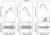 |
Fig. B.22 Corrected mode linewidth, mode height, and mode amplitude (top), and relative values of these parameters with respect to the reference fit (bottom) as a function of mode frequency for 12317678. The grey band indicates the range of systematic error around the reference fit values of ±15% for mode linewidth and mode height, of ±5% for mode amplitude. The error bars are those of the reference fit. |
Acknowledgments
We are grateful to the referee for the comments which considerably improved the structure and readability of the paper. The authors wish to thank the entire Kepler team, without whom these results would not have been possible. Funding for this Discovery mission is provided by NASA Science Mission Directorate. We also thank all funding councils and agencies that have supported the activities of KASC Working Group 1, as well as the International Space Science Institute (ISSI). T.A. gratefully acknowledges the financial support of the Centre National d’Etudes Spatiales (CNES) under a PLATO grant. T.L.C., W.J.C. and G.R.D. acknowledge financial support from the UK Science and Technology Facilities Council (STFC). Funding for the Stellar Astrophysics Centre is provided by The Danish National Research Foundation. The research is supported by the ASTERISK project (ASTERoseismic Investigations with SONG and Kepler) funded by the European Research Council (Grant agreement no.: 267864). R.A.G. and G.R.D. has received funding from the European Community Seventh Framework Programme (FP7/2007−2013) under grant agreement no. 269194. R.H. acknowledges computing support from the National Solar Observatory. SOHO is a mission of international collaboration between ESA and NASA. We thank Jérôme Ballot for useful discussions.
References
- Anderson, E. R., Duvall, T. L. J., & Jefferies, S. M. 1990, ApJ, 364, 699 [NASA ADS] [CrossRef] [Google Scholar]
- Appourchaux, T. 2011, A crash course on data analysis in asteroseismology, XXIIth Winter school of the Canary Islands [arXiv:1103.5352] [Google Scholar]
- Appourchaux, T., Andersen, B. N., Fröhlich, C., et al. 1997, Sol. Phys., 170, 27 [NASA ADS] [CrossRef] [Google Scholar]
- Appourchaux, T., Michel, E., Auvergne, M., et al. 2008, A&A, 488, 705 [NASA ADS] [CrossRef] [EDP Sciences] [Google Scholar]
- Appourchaux, T., Benomar, O., Gruberbauer, M., et al. 2012a, A&A, 537, A134 [NASA ADS] [CrossRef] [EDP Sciences] [Google Scholar]
- Appourchaux, T., Chaplin, W. J., García, R. A., et al. 2012b, A&A, 543, A54 [NASA ADS] [CrossRef] [EDP Sciences] [Google Scholar]
- Baglin, A. 2006, The CoRoT mission, pre-launch status, stellar seismology and planet finding, eds. M. Fridlund, A. Baglin, J. Lochard, & L.Conroy (Noordwijk, The Netherlands: ESA Publication Division), ESA SP-1306 [Google Scholar]
- Ballot, J., García, R. A., & Lambert, P. 2006, MNRAS, 369, 1281 [NASA ADS] [CrossRef] [Google Scholar]
- Ballot, J., Barban, C., & van’t Veer-Menneret, C. 2011, A&A, 531, A124 [NASA ADS] [CrossRef] [EDP Sciences] [Google Scholar]
- Balmforth, N. J. 1992, MNRAS, 255, 603 [NASA ADS] [CrossRef] [Google Scholar]
- Baudin, F., Barban, C., Belkacem, K., et al. 2011, A&A, 529, A84 [NASA ADS] [CrossRef] [EDP Sciences] [Google Scholar]
- Beck, P. G., Bedding, T. R., Mosser, B., et al. 2011, Science, 332, 205 [NASA ADS] [CrossRef] [PubMed] [Google Scholar]
- Beck, P. G., Montalban, J., Kallinger, T., et al. 2012, Nature, 481, 55 [NASA ADS] [CrossRef] [Google Scholar]
- Bedding, T. R., Mosser, B., Huber, D., et al. 2011, Nature, 471, 608 [NASA ADS] [CrossRef] [PubMed] [Google Scholar]
- Belkacem, K., Goupil, M. J., Dupret, M. A., et al. 2011, A&A, 530, A142 [NASA ADS] [CrossRef] [EDP Sciences] [Google Scholar]
- Belkacem, K., Dupret, M. A., Baudin, F., et al. 2012, A&A, 540, L7 [NASA ADS] [CrossRef] [EDP Sciences] [Google Scholar]
- Benomar, O., Appourchaux, T., & Baudin, F. 2009, A&A, 506, 15 [NASA ADS] [CrossRef] [EDP Sciences] [Google Scholar]
- Benomar, O., Bedding, T. R., Mosser, B., et al. 2013, ApJ, 767, 158 [NASA ADS] [CrossRef] [Google Scholar]
- Bruntt, H., Basu, S., Smalley, B., et al. 2012, MNRAS, 423, 122 [NASA ADS] [CrossRef] [Google Scholar]
- Chaplin, W. J., Elsworth, Y., Isaak, G. R., et al. 1997, MNRAS, 288, 623 [NASA ADS] [CrossRef] [Google Scholar]
- Chaplin, W. J., Elsworth, Y., Miller, B. A., New, R., & Verner, G. A. 2008, Sol. Phys., 251, 189 [NASA ADS] [CrossRef] [Google Scholar]
- Chaplin, W. J., Houdek, G., Karoff, C., Elsworth, Y., & New, R. 2009, A&A, 500, L21 [NASA ADS] [CrossRef] [EDP Sciences] [Google Scholar]
- Chaplin, W. J., Basu, S., Huber, D., et al. 2014, ApJS, 210, 1 [NASA ADS] [CrossRef] [Google Scholar]
- Corsaro, E., Stello, D., Huber, D., et al. 2012, ApJ, 757, 190 [NASA ADS] [CrossRef] [Google Scholar]
- Deheuvels, S., García, R. A., Chaplin, W. J., et al. 2012, ApJ, 756, 19 [NASA ADS] [CrossRef] [Google Scholar]
- Fletcher, S. T., Chaplin, W. J., Elsworth, Y., & New, R. 2009, ApJ, 694, 144 [NASA ADS] [CrossRef] [Google Scholar]
- Freytag, B., & Salaris, M. 1999, ApJ, 513, L49 [NASA ADS] [CrossRef] [Google Scholar]
- Fröhlich, C., Romero, J., Roth, H., et al. 1995, Sol. Phys., 162, 101 [NASA ADS] [CrossRef] [Google Scholar]
- Fröhlich, C., Andersen, B. N., Appourchaux, T., et al. 1997, in Sounding Solar and Stellar Interiors, eds. J. Provost, & F.-X. Schmider (Dordrecht Kluwer Academic Publishers), IAU Symp., 181, 67 [Google Scholar]
- García, R. A., Hekker, S., Stello, D., et al. 2011, MNRAS, 414, L6 [NASA ADS] [CrossRef] [Google Scholar]
- Gilliland, R. L., Jenkins, J. M., Borucki, W. J., et al. 2010, ApJ, 713, L160 [NASA ADS] [CrossRef] [Google Scholar]
- Gizon, L., & Solanki, S. K. 2003, ApJ, 589, 1009 [NASA ADS] [CrossRef] [Google Scholar]
- Goldreich, P., & Murray, N. 1994, ApJ, 424, 480 [NASA ADS] [CrossRef] [Google Scholar]
- Gough, D. 1980, in Nonradial and Nonlinear Stellar Pulsation, eds. H. A. Hill, & W. A. Dziembowski (Berlin Springer Verlag), Lect. Notes Phys., 125, 273 [Google Scholar]
- Handberg, R., & Campante, T. L. 2011, A&A, 527, A56 [NASA ADS] [CrossRef] [EDP Sciences] [Google Scholar]
- Harvey, J. 1985, in Future missions in solar, heliospheric and space plasma physics, eds. E. Rolfe, & B. Battrick (Noordwijk, The Netherlands: ESA Publications Division), ESA SP, 235, 199 [Google Scholar]
- Houdek, G. 1996, Ph.D. Thesis, Univeristät Wien [Google Scholar]
- Houdek, G., Balmforth, N. J., Christensen-Dalsgaard, J., & Gough, D. O. 1999, A&A, 351, 582 [NASA ADS] [Google Scholar]
- Houdek, G., Chaplin, W. J., Appourchaux, T., et al. 2001, MNRAS, 327, 483 [NASA ADS] [CrossRef] [Google Scholar]
- Howe, R., & Hill, F. 1998, in Structure and Dynamics of the Interior of the Sun and Sun-like Stars, ed. S. Korzennik, & A. Wilson (Noordwijk, The Netherlands: ESA Publications Division), ESA SP, 418, 237 [Google Scholar]
- Jenkins, J. M., Caldwell, D. A., Chandrasekaran, H., et al. 2010, ApJ, 713, L87 [NASA ADS] [CrossRef] [Google Scholar]
- Karoff, C., Metcalfe, T. S., Chaplin, W. J., et al. 2013, MNRAS, 433, 3227 [NASA ADS] [CrossRef] [Google Scholar]
- Kjeldsen, H., & Bedding, T. R. 1995, A&A, 293, 87 [NASA ADS] [Google Scholar]
- Komm, R. W., Howe, R., & Hill, F. 2000, ApJ, 543, 472 [NASA ADS] [CrossRef] [Google Scholar]
- Libbrecht, K. G. 1988, ApJ, 334, 510 [NASA ADS] [CrossRef] [Google Scholar]
- Ludwig, H.-G., Freytag, B., & Steffen, M. 1999, A&A, 346, 111 [NASA ADS] [Google Scholar]
- Mosser, B., Goupil, M. J., Belkacem, K., et al. 2012a, A&A, 548, A10 [NASA ADS] [CrossRef] [EDP Sciences] [Google Scholar]
- Mosser, B., Goupil, M. J., Belkacem, K., et al. 2012b, A&A, 540, A143 [NASA ADS] [CrossRef] [EDP Sciences] [Google Scholar]
- Muller, R., Hanslmeier, A., & Saldaña-Muñoz, M. 2007, A&A, 475, 717 [NASA ADS] [CrossRef] [EDP Sciences] [Google Scholar]
- Muller, R., Utz, D., & Hanslmeier, A. 2011, Sol. Phys., 274, 87 [NASA ADS] [CrossRef] [Google Scholar]
- Pinheiro, F. J. G., & Fernandes, J. 2013, MNRAS, 433, 2893 [NASA ADS] [CrossRef] [Google Scholar]
- Pinsonneault, M. H., An, D., Molenda-Żakowicz, J., et al. 2012, ApJS, 199, 30 [NASA ADS] [CrossRef] [Google Scholar]
- Salabert, D., Ballot, J., & García, R. A. 2011, A&A, 528, A25 [Google Scholar]
- Samadi, R. 2011, in Lect. Notes Phys. 832, eds. J.-P. Rozelot, & C. Neiner (Berlin Springer Verlag), 305 [Google Scholar]
- Scargle, J. D. 1982, ApJ, 263, 835 [NASA ADS] [CrossRef] [Google Scholar]
- Toutain, T., & Appourchaux, T. 1994, A&A, 289, 649 [NASA ADS] [Google Scholar]
- Toutain, T., Elsworth, Y., & Chaplin, W. J. 2005, A&A, 433, 713 [NASA ADS] [CrossRef] [EDP Sciences] [Google Scholar]
- Trampedach, R., & Stein, R. F. 2011, ApJ, 731, 78 [NASA ADS] [CrossRef] [Google Scholar]
- Vaughan, A. H., & Preston, G. W. 1980, PASP, 92, 385 [NASA ADS] [CrossRef] [Google Scholar]
All Tables
Model parameters affecting directly the stellar background, mode linewidth, and mode height.
All Figures
|
Fig. 1 Mode linewidth, mode height and mode amplitude (top), and relative values of these parameters with respect to the reference fit (bottom) as a function of mode frequency for various fitters for KIC 3733735. The grey band indicates the range of systematic error around the reference fit values of ±15% for mode linewidth and mode height, of ±5% for mode amplitude. The 1-σ error bars are those of Appourchaux. |
| In the text | |
|
Fig. 2 Corrected mode linewidth, mode height, and mode amplitude (top), and relative values of these parameters with respect to the reference fit (bottom) as a function of mode frequency for KIC 3733735. The grey band indicates the range of systematic error around the reference fit values of ±15% for mode linewidth and mode height, of ±5% for mode amplitude. The error bars are those of the reference fit. |
| In the text | |
|
Fig. 3 Mode linewidth as a function of the mode order for the 23 stars with their colour identified by their effective temperature, for the l = 0 mode linewidths of 4 sub-giant stars of Benomar et al. (2013) (dashed lines), and for the solar LOI data (solid black line). For the 23 stars of this study the relative 1-σ error bars range from 5% to 10%, while those of Benomar et al. (2013) range from 10% to 20%. The 10% and 20% error bars are shown as an example. The longer LOI data set has relative error bars of about 2%. |
| In the text | |
|
Fig. 4 Mode height and amplitude as a function of the mode order for the 23 stars with their colour identified by their effective temperature (as in Fig. 3), for the 4 sub-giant stars of Benomar et al. (2013) (dashed lines), and for the solar LOI data (solid black line). The relative 1-σ error bars for mode height are similar to those of the mode linewidth, while they are typically 3 times smaller for mode amplitude. |
| In the text | |
|
Fig. 5 Mode linewidth as a function of frequency for KIC 6116048 (solid line) with its 1-σ error bars compared with the fit following Eq. (1) (orange line). |
| In the text | |
|
Fig. 6 Parameters of Eq. (1) as a function of the effective temperature for all 28 stars, for the power law dependence (left) and for the Lorentzian fit (right). The median value together with the credible intervals at 33% and 66% were derived from a Monte-Carlo simulation of the fit. The orange line shows the temperature dependence of the linewidth at the frequency of maximum mode height as derived by Appourchaux et al. (2012a). The open diamond is the result of the fit for the solar data of the LOI. The open triangles are the results of the fit for the sub-giant stars of Benomar et al. (2013). The solid lines show a linear fit of the parameters with respect to the effective temperature. The Lorentzian parameters for stars for which the Lorentzian fit is not significant are not plotted. |
| In the text | |
|
Fig. 7 Parameters of Eq. (1) as a function of the frequency of maximum mode height for all 28 stars, for the power law dependence (left) and for the Lorentzian fit (right). The median value together with the credible intervals of 33% and 66% were derived from a Monte-Carlo simulation of the fit. The open diamond is the result of the fit for the solar LOI data. The open triangles are the result of the fit for the sub-giant stars of Benomar et al. (2013). The error bars are derived from a Monte-Carlo simulation using credible intervals of 33% and 66%. The solid lines show a linear fit of the parameters with respect to the frequency. The Lorentzian parameters for stars for which the Lorentzian fit is not significant are not plotted. |
| In the text | |
|
Fig. A.1 Mode parameter biases as a function of linewidth for a stellar background bias of +1%, for several signal-to-noise ratios and for three different kinds of profiles which are: a triplet l = 0,1,2,3 with a splitting of 2 μHz with the mode pairs l = 0 − 2 and l = 1 − 3 separated by 120 μHz (black line); a triplet with a splitting of 6 μHz with the mode pair l = 0 − 2 and l = 1 − 3 separated by 120 μHz (green line); and a single mode profile (red line). (Top, left) For mode linewidth, (top, right) For mode height ratio, (bottom, left) For mode amplitude. |
| In the text | |
|
Fig. A.2 Relative systematic error of three parameters of the l = 0 − 2 and l = 1 − 3 modes as a function of the fitted splitting: mode linewidth (solid line), mode height (dotted line), mode amplitude (dashed line) for a signal-to-noise ratio of 1, a nominal splitting of 4 μHz and an inclination angle of 90 degrees. Left: the multiplet has a nominal linewidth of 6 μHz. Right: the multiplet has a nominal linewidth of 3 μHz. |
| In the text | |
|
Fig. A.3 Relative systematic error of three parameters of the l = 0 − 2 and l = 1 − 3 modes as a function of the fitted splitting: mode linewidth (solid line), mode height (dotted line), mode amplitude (dashed line) for a signal-to-noise ratio of 1, a nominal splitting of 0.4 μHz and an inclination angle of 90 degrees. Left: the multiplet has a nominal linewidth of 3 μHz. Right: the multiplet has a nominal linewidth of 1 μHz. |
| In the text | |
|
Fig. A.4 Relative systematic error on three parameters of the l = 0 − 2 and l = 1 − 3 multiplet as function of the fitted inclination angle: mode linewidth (solid line), mode height (dotted line), mode amplitude (dashed line) for a signal-to-noise ratio of 1. The multiplet has a nominal linewidth of 6 μHz and a nominal splitting of 4 μHz, with a nominal inclination angle of 45 degrees (left), and a nominal inclination angle of 90 degrees (right). |
| In the text | |
|
Fig. A.5 Relative systematic error as a function of the deviation to the reference mode visibility for the mode height (black line) and linewidth (orange line) for a set of l = 0,1,2 modes with a 2-μHz linewidth, and a signal-to-noise ratio 10 for the l = 0 mode. The continuous lines are the systematic error computed using the method of Toutain et al. (2005). The dashed line is the analytical systematic error on mode height derived assuming there is no systematic error on the linewidth derived from Eq. (B.38). Top left: the deviations to the reference mode visibilities are identical for l = 1 and l = 2. Bottom left: the deviations to the reference mode visibilities are of opposite sign for l = 1 and l = 2. Top right: the deviation to the reference mode visibilities is zero for l = 2. Bottom right: the deviation to the reference mode visibilities is zero for l = 1. |
| In the text | |
|
Fig. A.6 Relative systematic error as a function of frequency for a mean frequency shifted by half the large separation for the solar case for mode linewidth (left) and for mode height (right) using BiSON data (black line, Chaplin et al. 1997) and GONG data (orange line, Komm et al. 2000). |
| In the text | |
|
Fig. B.1 Corrected mode linewidth, mode height, and mode amplitude (top), and relative values of these parameters with respect to the reference fit (bottom) as a function of mode frequency for KIC 1435467. The grey band indicates the range of systematic error around the reference fit values of ±15% for mode linewidth and mode height, of ±5% for mode amplitude. The error bars are those of the reference fit. |
| In the text | |
|
Fig. B.2 Corrected mode linewidth, mode height, and mode amplitude (top), and relative values of these parameters with respect to the reference fit (bottom) as a function of mode frequency for KIC 2837475. The grey band indicates the range of systematic error around the reference fit values of ±15% for mode linewidth and mode height, of ±5% for mode amplitude. The error bars are those of the reference fit. |
| In the text | |
|
Fig. B.3 Corrected mode linewidth, mode height, and mode amplitude (top), and relative values of these parameters with respect to the reference fit (bottom) as a function of mode frequency for KIC 3424541. The grey band indicates the range of systematic error around the reference fit values of ±15% for mode linewidth and mode height, of ±5% for mode amplitude. The error bars are those of the reference fit. |
| In the text | |
|
Fig. B.4 Corrected mode linewidth, mode height, and mode amplitude (top), and relative values of these parameters with respect to the reference fit (bottom) as a function of mode frequency for KIC 6116048. The grey band indicates the range of systematic error around the reference fit values of ±15% for mode linewidth and mode height, of ±5% for mode amplitude. The error bars are those of the reference fit. |
| In the text | |
|
Fig. B.5 Corrected mode linewidth, mode height, and mode amplitude (top), and relative values of these parameters with respect to the reference fit (bottom) as a function of mode frequency for KIC 6508366. The grey band indicates the range of systematic error around the reference fit values of ±15% for mode linewidth and mode height, of ±5% for mode amplitude. The error bars are those of the reference fit. |
| In the text | |
|
Fig. B.6 Corrected mode linewidth, mode height, and mode amplitude (top), and relative values of these parameters with respect to the reference fit (bottom) as a function of mode frequency for KIC 6679371. The grey band indicates the range of systematic error around the reference fit values of ±15% for mode linewidth and mode height, of ±5% for mode amplitude. The error bars are those of the reference fit. |
| In the text | |
|
Fig. B.7 Corrected mode linewidth, mode height, and mode amplitude (top), and relative values of these parameters with respect to the reference fit (bottom) as a function of mode frequency for KIC 7103006. The grey band indicates the range of systematic error around the reference fit values of ±15% for mode linewidth and mode height, of ±5% for mode amplitude. The error bars are those of the reference fit. |
| In the text | |
|
Fig. B.8 Corrected mode linewidth, mode height, and mode amplitude (top), and relative values of these parameters with respect to the reference fit (bottom) as a function of mode frequency for KIC 7206837. The grey band indicates the range of systematic error around the reference fit values of ±15% for mode linewidth and mode height, of ±5% for mode amplitude. The error bars are those of the reference fit. |
| In the text | |
|
Fig. B.9 Corrected mode linewidth, mode height, and mode amplitude (top), and relative values of these parameters with respect to the reference fit (bottom) as a function of mode frequency for KIC 8379927. The grey band indicates the range of systematic error around the reference fit values of ±15% for mode linewidth and mode height, of ±5% for mode amplitude. The error bars are those of the reference fit. |
| In the text | |
|
Fig. B.10 Corrected mode linewidth, mode height, and mode amplitude (top), and relative values of these parameters with respect to the reference fit (bottom) as a function of mode frequency for KIC 8694723. The grey band indicates the range of systematic error around the reference fit values of ±15% for mode linewidth and mode height, of ±5% for mode amplitude. The error bars are those of the reference fit. |
| In the text | |
|
Fig. B.11 Corrected mode linewidth, mode height, and mode amplitude (top), and relative values of these parameters with respect to the reference fit (bottom) as a function of mode frequency for KIC 9139151. The grey band indicates the range of systematic error around the reference fit values of ±15% for mode linewidth and mode height, of ±5% for mode amplitude. The error bars are those of the reference fit. |
| In the text | |
|
Fig. B.12 Corrected mode linewidth, mode height, and mode amplitude (top), and relative values of these parameters with respect to the reference fit (bottom) as a function of mode frequency for KIC 9139163. The grey band indicates the range of systematic error around the reference fit values of ±15% for mode linewidth and mode height, of ±5% for mode amplitude. The error bars are those of the reference fit. |
| In the text | |
|
Fig. B.13 Corrected mode linewidth, mode height, and mode amplitude (top), and relative values of these parameters with respect to the reference fit (bottom) as a function of mode frequency for KIC 9206432. The grey band indicates the range of systematic error around the reference fit values of ±15% for mode linewidth and mode height, of ±5% for mode amplitude. The error bars are those of the reference fit. |
| In the text | |
|
Fig. B.14 Corrected mode linewidth, mode height, and mode amplitude (top), and relative values of these parameters with respect to the reference fit (bottom) as a function of mode frequency for KIC 9812850. The grey band indicates the range of systematic error around the reference fit values of ±15% for mode linewidth and mode height, of ±5% for mode amplitude. The error bars are those of the reference fit. |
| In the text | |
|
Fig. B.15 Corrected mode linewidth, mode height, and mode amplitude (top), and relative values of these parameters with respect to the reference fit (bottom) as a function of mode frequency for KIC 10162436. The grey band indicates the range of systematic error around the reference fit values of ±15% for mode linewidth and mode height, of ±5% for mode amplitude. The error bars are those of the reference fit. |
| In the text | |
|
Fig. B.16 Corrected mode linewidth, mode height, and mode amplitude (top), and relative values of these parameters with respect to the reference fit (bottom) as a function of mode frequency for KIC 10355856. The grey band indicates the range of systematic error around the reference fit values of ±15% for mode linewidth and mode height, of ±5% for mode amplitude. The error bars are those of the reference fit. |
| In the text | |
|
Fig. B.17 Corrected mode linewidth, mode height, and mode amplitude (top), and relative values of these parameters with respect to the reference fit (bottom) as a function of mode frequency for KIC 10454113. The grey band indicates the range of systematic error around the reference fit values of ±15% for mode linewidth and mode height, of ±5% for mode amplitude. The error bars are those of the reference fit. |
| In the text | |
|
Fig. B.18 Corrected mode linewidth, mode height, and mode amplitude (top), and relative values of these parameters with respect to the reference fit (bottom) as a function of mode frequency for KIC 10909629. The grey band indicates the range of systematic error around the reference fit values of ±15% for mode linewidth and mode height, of ±5% for mode amplitude. The error bars are those of the reference fit. |
| In the text | |
|
Fig. B.19 Corrected mode linewidth, mode height, and mode amplitude (top), and relative values of these parameters with respect to the reference fit (bottom) as a function of mode frequency for 11081729. The grey band indicates the range of systematic error around the reference fit values of ±15% for mode linewidth and mode height, of ±5% for mode amplitude. The error bars are those of the reference fit. |
| In the text | |
|
Fig. B.20 Corrected mode linewidth, mode height, and mode amplitude (top), and relative values of these parameters with respect to the reference fit (bottom) as a function of mode frequency for 12009504. The grey band indicates the range of systematic error around the reference fit values of ±15% for mode linewidth and mode height, of ±5% for mode amplitude. The error bars are those of the reference fit. |
| In the text | |
|
Fig. B.21 Corrected mode linewidth, mode height, and mode amplitude (top), and relative values of these parameters with respect to the reference fit (bottom) as a function of mode frequency for 12258514. The grey band indicates the range of systematic error around the reference fit values of ±15% for mode linewidth and mode height, of ±5% for mode amplitude. The error bars are those of the reference fit. |
| In the text | |
|
Fig. B.22 Corrected mode linewidth, mode height, and mode amplitude (top), and relative values of these parameters with respect to the reference fit (bottom) as a function of mode frequency for 12317678. The grey band indicates the range of systematic error around the reference fit values of ±15% for mode linewidth and mode height, of ±5% for mode amplitude. The error bars are those of the reference fit. |
| In the text | |
Current usage metrics show cumulative count of Article Views (full-text article views including HTML views, PDF and ePub downloads, according to the available data) and Abstracts Views on Vision4Press platform.
Data correspond to usage on the plateform after 2015. The current usage metrics is available 48-96 hours after online publication and is updated daily on week days.
Initial download of the metrics may take a while.