| Issue |
A&A
Volume 566, June 2014
|
|
|---|---|---|
| Article Number | A20 | |
| Number of page(s) | 35 | |
| Section | Stellar structure and evolution | |
| DOI | https://doi.org/10.1051/0004-6361/201323317 | |
| Published online | 02 June 2014 | |
Online material
Mode heights, mode linewidths and mode amplitude for KIC 1435467.
Mode heights, mode linewidths and mode amplitude for KIC 2837475.
Mode heights, mode linewidths and mode amplitude for KIC 3424541.
Mode heights, mode linewidths and mode amplitude for KIC 3733735.
Mode heights, mode linewidths and mode amplitude for KIC 6116048.
Mode heights, mode linewidths and mode amplitude for KIC 6508366.
Mode heights, mode linewidths and mode amplitude for KIC 6679371.
Mode heights, mode linewidths and mode amplitude for KIC 7103006.
Mode heights, mode linewidths and mode amplitude for KIC 7206837.
Mode heights, mode linewidths and mode amplitude for KIC 8379927.
Mode heights, mode linewidths and mode amplitude for KIC 8694723.
Mode heights, mode linewidths and mode amplitude for KIC 9139151.
Mode heights, mode linewidths and mode amplitude for KIC 9139163.
Mode heights, mode linewidths and mode amplitude for KIC 9206432.
Mode heights, mode linewidths and mode amplitude for KIC 9812850.
Mode heights, mode linewidths and mode amplitude for KIC 10162436.
Mode heights, mode linewidths and mode amplitude for KIC 10162436.
Mode heights, mode linewidths and mode amplitude for KIC 10355856.
Mode heights, mode linewidths and mode amplitude for KIC 10454113.
Mode heights, mode linewidths and mode amplitude for KIC 10909629.
Mode linewidths, mode heights and mode amplitude for KIC 11081729.
Mode linewidths, mode heights and mode amplitude for KIC 12009504.
Mode linewidths, mode heights and mode amplitude for KIC 12258514
Mode linewidths, mode heights and mode amplitude for KIC 12317678.
Appendix A: Source of systematic errors and their correction
In this appendix, we mainly focus on internal differences resulting from different fit assumptions, which led to different fitted results. The observation duration, being common to all fitters, was excluded from the possible source of systematic errors; in addition since the observation duration was larger than 30 times the longest mode lifetime (see Chaplin et al. 2008) this source of external systematic error was negligible. We also note, that the values of mode linewidths, and mode heights obtained with MLE are derived from the mean value of the natural logarithm of these parameters, while the Bayesian values are obtained from the median of these parameters (Benomar et al. 2009), resulting in differences between the two statistical values of less than a few percent, thanks to the long observation duration.
The large deviations between the results obtained leads to an investigation of the possible sources of systematic errors, which are:
-
Bias on the estimated stellar background.
-
Bias on the estimated splitting and inclination angle.
-
Bias on the assumed mode height ratio.
-
Different definition of the mean frequency.
Hereafter we detail each source of systematic error from a theoretical and practical point of view. The theoretical understanding of the systematic errors is based on the use of MLE for mode extraction. Other extracting methods used in this paper derive the mode parameters in a Bayesian framework (Benomar et al. 2009; Handberg & Campante 2011). The two methods are obviously not identical since the Bayesian approach used a priori information on the parameters to be fitted which will slant the outcome in a different manner. We deliberately chose not to take account of these additional systematic errors, which are far more difficult to model than those resulting from using the MLE approach. The correction approach based upon an MLE fit proved its efficacy, showing that there was no need to take into account the Bayesian parameter derivation in the correction scheme.
Table A.1 lists the model characteristics of each fitter whose differences lead to systematic errors in the mode linewidth and height.
Model parameters affecting directly the stellar background, mode linewidth, and mode height.
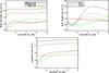 |
Fig. A.1
Mode parameter biases as a function of linewidth for a stellar background bias of +1%, for several signal-to-noise ratios and for three different kinds of profiles which are: a triplet l = 0,1,2,3 with a splitting of 2 μHz with the mode pairs l = 0 − 2 and l = 1 − 3 separated by 120 μHz (black line); a triplet with a splitting of 6 μHz with the mode pair l = 0 − 2 and l = 1 − 3 separated by 120 μHz (green line); and a single mode profile (red line). (Top, left) For mode linewidth, (top, right) For mode height ratio, (bottom, left) For mode amplitude. |
| Open with DEXTER | |
Appendix A.1: Effect of an incorrect estimation of the stellar background
One might naively assume that an underestimated stellar background would lead to an overestimated mode height compensating the reduced stellar background. This naive approach would provide an underestimated linewidth. Fortunately, the effect of an incorrect estimation of the stellar background on the mode can be analytically calculated which provides a counter intuitive result. The relations between the mode-linewidth, mode-height and mode-amplitude systematic errors which lead to an incorrect estimated stellar background are given in Appendix B.2. In short, an underestimation of the stellar background will lead to an underestimation of the mode height and an overestimation of the linewidth. In addition, the lower the signal-to-noise ratio the higher the systematic error on mode linewidth and height (the signal-to-noise ratio is the ratio of mode height to the stellar background). The systematic errors were also numerically derived using the technique of the fit of a single (not many) profile of Toutain et al. (2005), i.e. by simulation of the MLE for a single profile fitted by a profile with a different stellar background. Figure A.1 shows the results of the numerical calculation of the mode linewidth, mode height, and mode amplitudes biases as a function of mode linewidth, for several signal-to-noise ratio. Assuming that the background is overestimated by 1%, then when the signal-to-noise ratio is about 10, the mode linewidth is typically underestimated by about 1.75%, while the mode height is overestimated by about 0.75 %. The sign of the mode-linewidth systematic error is opposite to that of the mode-height systematic error, such that they almost compensate each other when computing the mode-amplitude systematic errors. It means that an overestimation of the stellar background of 1% will provide a mode amplitude underestimated by 0.5%.
When the signal-to-noise ratio is close to 1, the mode-linewidth systematic errors increases to about −8% while the mode-height systematic errors are only 2%. This is what was observed in some stars for which we could not understand why the systematic error on the linewidth was so much larger than for the mode height. As a consequence, care should be taken when comparing amplitudes of different fitters when the signal-to-noise ratio is low.
We also note that when the signal-to-noise ratio increases, the mode-amplitude systematic error gets smaller and smaller, i.e. a 1% stellar background overestimation would provide a 0.1% mode amplitude underestimation. This explains why the mode amplitude differences between different fits may be very small but not necessarily absent when the signal-to-noise ratio is high.
The differences between the different fitted stellar backgrounds can vary between 30% in the worst case to about 10% in the best cases. The differences are mainly due to the model of the stellar background used having one or several components as shown in Table A.1. It must be pointed out that since the background bias varies with frequency, this will also introduce a varying effect on the relative variation of the mode linewidth and mode height.
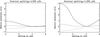 |
Fig. A.2
Relative systematic error of three parameters of the l = 0 − 2 and l = 1 − 3 modes as a function of the fitted splitting: mode linewidth (solid line), mode height (dotted line), mode amplitude (dashed line) for a signal-to-noise ratio of 1, a nominal splitting of 4 μHz and an inclination angle of 90 degrees. Left: the multiplet has a nominal linewidth of 6 μHz. Right: the multiplet has a nominal linewidth of 3 μHz. |
| Open with DEXTER | |
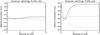 |
Fig. A.3
Relative systematic error of three parameters of the l = 0 − 2 and l = 1 − 3 modes as a function of the fitted splitting: mode linewidth (solid line), mode height (dotted line), mode amplitude (dashed line) for a signal-to-noise ratio of 1, a nominal splitting of 0.4 μHz and an inclination angle of 90 degrees. Left: the multiplet has a nominal linewidth of 3 μHz. Right: the multiplet has a nominal linewidth of 1 μHz. |
| Open with DEXTER | |
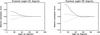 |
Fig. A.4
Relative systematic error on three parameters of the l = 0 − 2 and l = 1 − 3 multiplet as function of the fitted inclination angle: mode linewidth (solid line), mode height (dotted line), mode amplitude (dashed line) for a signal-to-noise ratio of 1. The multiplet has a nominal linewidth of 6 μHz and a nominal splitting of 4 μHz, with a nominal inclination angle of 45 degrees (left), and a nominal inclination angle of 90 degrees (right). |
| Open with DEXTER | |
Appendix A.2: Effect of a different estimated splitting and inclination angle
The effect of a different estimated splitting can also be simply understood when, for example, a null splitting is fitted when the modes are genuinely split: this will lead to an overestimation of the linewidth. The analytical calculations of the effect are detailed in Appendix B.3 but do not lead to simple useful formula; the only result being that second order effects dominate. This is the reason why we simulated an l = 0 − 2 pair and an l = 1 − 3 pair with a symmetrical rotational splitting and with mode height ratio of 1/1.5/0.5/0.05 for the l = 0,1,2,3, respectively. We then applied the one-fit method of Toutain et al. (2005) for computing the systematic errors. Figures A.2 to A.4 show results for three different cases.
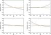 |
Fig. A.5
Relative systematic error as a function of the deviation to the reference mode visibility for the mode height (black line) and linewidth (orange line) for a set of l = 0,1,2 modes with a 2-μHz linewidth, and a signal-to-noise ratio 10 for the l = 0 mode. The continuous lines are the systematic error computed using the method of Toutain et al. (2005). The dashed line is the analytical systematic error on mode height derived assuming there is no systematic error on the linewidth derived from Eq. (B.38). Top left: the deviations to the reference mode visibilities are identical for l = 1 and l = 2. Bottom left: the deviations to the reference mode visibilities are of opposite sign for l = 1 and l = 2. Top right: the deviation to the reference mode visibilities is zero for l = 2. Bottom right: the deviation to the reference mode visibilities is zero for l = 1. |
| Open with DEXTER | |
In Fig. A.2, for a 90-degree inclination (perpendicular to the line of sight), when the nominal splitting is of the order of the linewidth, the fitted linewidth with a null fitted splitting will be typically overestimated by the value in excess of a few times the nominal splitting. In Fig. A.3, for a 90-degree inclination (perpendicular to the line of sight), when the nominal splitting is about 10% to 20% of the linewidth, the fitted linewidth with a null fitted splitting will be typically overestimated by the value smaller than the nominal splitting. We also note that the dependence of the linewidth bias on to the splitting is quadratic close to the nominal splitting but not exactly at the nominal splitting. At the local minimum, the systematic error is slightly negative, although the systematic error at the nominal splitting is null.
In Fig. A.4, we also simulated a varying inclination, assuming that the projected splitting was kept constant ( ). The reason for using such a formulation is that the fit preferentially converges towards a value for which
  is constant as shown by Ballot et al. (2006). The systematic errors remain small when the fitted inclination angle is greater than 45 degrees. In addition the systematic errors decrease with the inclination angle. Therefore a correction is clearly necessary when the fitted inclination angles are less than 45 degrees while the fitted reference inclination angle is above 45 degrees, i.e. a difference of about 45 degrees will produce large systematic errors in the mode parameters.
If one assumes the same splitting and inclination angle for all modes, the splitting and angle systematic errors introduce a frequency dependence on the relative variation of the mode linewidth and mode height when compared to the reference fit values. The frequency dependences on the relative errors are larger at smaller linewidths, emphasising the need for a proper estimation of the splitting at the low-frequency part of the spectrum.
Appendix A.3: Effect of different assumptions on mode height ratio
Some fitters also allow the mode height ratio to vary, which will also lead, when compared to the results obtained with a notional mode height ratio, to some systematic error in the measured linewidth and mode height. Neglecting the systematic error on mode linewidth, we analytically computed the systematic error on mode height (see Appendix B.4). We also applied the one-fit method of Toutain et al. (2005) for computing the systematic errors. Figure A.5 shows the results of the analytical and numerical calculations of the systematic errors on mode linewidth, mode height, and mode amplitudes biases as a function of deviations to the reference mode height ratio for a set of l = 0,1,2 modes with a 2-μHz linewidth, and a signal-to-noise ratio of 10 for the l = 0 mode.
To first order, the impact of a different mode height ratio on the linewidth is rather small and typically of the order of 10%. On the other hand, the impact of a different mode height ratio is much larger on the mode height, being close to 40% in the worst case. In addition, the systematic error on the mode height ratio will produce a non-negligible systematic error on the mode amplitude. Ballot et al. (2011) showed, using adiabatic computations, that the mode height ratio varies with the effective temperature, surface gravity, and metallicity. For the stars listed in this study, using the work of Ballot et al. (2011) and the stellar parameters provided by Bruntt et al. (2012) we derived that the mode height ratio for l = 1, l = 2, l = 3 is 1.5, 0.52, 0.025 varying by 0.02, 0.02, 0.004, respectively.
As shown by Salabert et al. (2011) for the solar case, the measured ratios agree very well with the theoretical ratios to within 0.06 and do not vary with time. Such a deviation of 0.06 would result in systematic errors not larger than 4% for the mode height, a value that can also be derived from Eq. (B.38). The values derived above from Ballot et al. (2011) would provide even a smaller systematic error not larger than 2%. Larger deviations of stellar mode ratio with respect to the value given above were also observed (Salabert 2013, priv. comm.). At the time of writing, given that the variation of the mode height ratio is primarily geometrical, there is very little variation with mode frequency. Then, in order to achieve a repeatable measurement, it is advised to keep the mode height ratio at reference values of 1.5, 0.5, 0.05 for l = 1, l = 2, and l = 3, respectively.
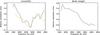 |
Fig. A.6
Relative systematic error as a function of frequency for a mean frequency shifted by half the large separation for the solar case for mode linewidth (left) and for mode height (right) using BiSON data (black line, Chaplin et al. 1997) and GONG data (orange line, Komm et al. 2000). |
| Open with DEXTER | |
Appendix A.4: Effect of a different definition of mean frequency
By definition of the model, the linewidth is set to be common for modes that are within half a large separation. There are two possible configurations defining for which modes the linewidth will be common: configuration A for which the l = 0,2 mode pair is at the left of the l = 1 mode; and configuration B for which the l = 0,2 mode pair is at the right of the l = 1 mode. As a result, the mean frequency will differ for the different configurations. For configuration A, the mean frequency is νn,0 + Δν/ 4, while for configuration B, it is νn,0 − Δν/ 4. Therefore depending on how the fits are performed there could be up to a Δν/ 2 difference in the mean frequency. Since it is assumed that the mode linewidth only depends upon mode frequency, this would directly produce a systematic error that would be proportional to the linewidth frequency derivative and the frequency difference.
Figure A.6 shows the resulting relative systematic error on mode linewidth and mode height in the solar case using BiSON and GONG data. The relative error could be up to 40% especially at the low frequencies. Fortunately, the signal-to-noise ratio of the Kepler observations allows the observation of low order modes only for stars more massive than the Sun having higher mode amplitude. These stars then have smaller large separation than the Sun, typically about the third of the solar case. Therefore the relative error due to the different mean frequency is never larger than 10% for either the mode linewidth or the mode height.
Finally, only one fitter (Howe) used the formal order definition for which the l = 2 mode is separated by a large separation of the l = 0 mode of the same order n (configuration a in Table A.1). The problem of using this formal definition for fitting across a large separation is that the l = 2 mode of order n is very close to the l = 0 mode of order n + 1. In practice, then the formal order definition is almost never used for mode fitting. In any case, the difference of mean frequency of configuration A with respect to the formal order definition is then only Δν/ 4. It means that the systematics, resulting from the different definition in that case, are twice as small as those resulting from using configuration B, or less than 5%.
Appendix A.5: Implementation of the correction of the systematic errors
For each fit, the correction was computed by modelling the l = 0 − 2 and l = 1 − 3 modes over a window as large as the large separation (Δν) with the pair of modes separated by half of that. The large separation is 240 μHz. The l = 2 and l = 3 modes are assumed to be 6 μHz and 10 μHz to the left of their adjacent l = 0 or l = 1 mode. The correction could have been implemented with the proper large separation for each star but the results shows that the correction works even with the default large separation we used. The mode height ratios are assumed to be either 1.0/1.5/0.5/0.05 or 1.0/2.0/1.0/0.0, depending on the star or the fitter. The latter mode height ratio were typical results obtained by some fitters when freeing the ratios. The linewidth is common to the set of mode frequencies following configuration A. We note that the differences in the mean frequency between the different configurations were not implemented in the correction because of the rather small biases introduced. The stellar background is flat. The profile is modelled using the reference fit with the measured linewidth, mode height, splitting, inclination angle and stellar background. Since the value of the background is taken at the l = 0 mode, we neglect the frequency dependence of the stellar background within a large separation. In the worst case the differential variation of the fitted stellar background with respect to the reference fit is typically less than 0.5% across a large separation which is negligible compared to other systematic errors. The fit is performed for only the linewidth and mode height as free parameters with a fixed splitting, inclination angle, and stellar background provided by each fitter using the one-fit approach of Toutain et al. (2005). Finally, the correction of the systematic errors is computed by taking the ratio of the fitted linewidth or mode height to that of the reference fit.
We emphasize that the correction scheme could have been improved by using the mode-frequency configuration of each fitter, the true fitted mode height ratio of each mode or of the ensemble of modes and a non-flat stellar background. The simple correction scheme is sufficiently efficient to argue against making the correction model more complex.
Figures B.1 to B.22 show for the remaining 22 stars the mode linewidth, height, and amplitude corrected for systematic errors using the procedure described above.
Appendix B: Analytical derivation of the biases leading to systematic errors
Appendix B.1: Assumptions
The mode parameters are usually extracted from the power spectra using MLE which consists in finding the maximum of the following figure of merit (See Toutain & Appourchaux 1994, for details): 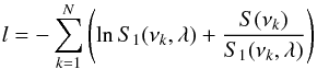 (B.1)where S1 is the model of the power spectra, S(νk) represents the spectral data at the frequency bin νk, λ is the vector of parameters (frequency, splitting, linewidth, etc.). In order to find the maximum of Eq. (B.1), one needs to compute the derivative with respect to λ. At the maximum, the derivative should be zero for all values of the element of the vector λ:
 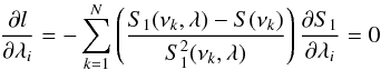 (B.2)which can be approximated, as per Toutain & Appourchaux (1994), by:
 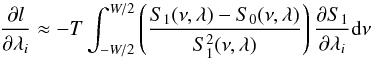 (B.3)where ν is the frequency, W is the frequency range over which the maximization is performed, T is the observation duration and S0 is the asymptotic mean spectra.
The procedure used for analytically finding the systematic errors is then simply to use the fact that  for all λi. The analytical derivation can then be compared with the one-fit approach of Toutain et al. (2005), which explicitly assumes that the bias obtained by fitting an observed spectrum S(ν) with a profile S1(ν,λ) is the same as fitting the asymptotic noiseless profile S0(ν,λ). The procedure used by Toutain et al. (2005) is then simply to fit S0(ν,λ) once instead of doing Monte-Carlo simulations of many realisation of S(ν). With this procedure, this is exactly the asymptotic expression of Eq. (B.1) that one maximises, which results in finding asymptotically the zero of
  as a function of the parameters λi.
In all of the following subsections, we assumed a symmetrical Lorentzian profile for the asymptotic and fitted profiles.
Appendix B.2: Effect of an incorrect estimation of the stellar background
When the fitted spectra S1 is different from S0, we can write to first order: 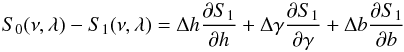 (B.4)where γ = lnΓ, h = lnH, b = lnB with Γ, H, and B being the mode linewidth, the mode height and the stellar background, respectively. We note that if we assume that the model of the mode profile includes a white noise background, we have
  . Inserting Eqs. (B.4) in (B.3), one gets for the derivative with respect to γ and h:
 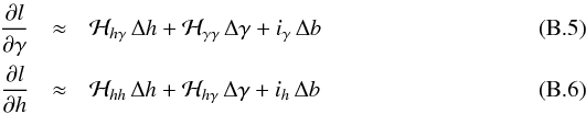 where ℋhγ, ℋγγ and ℋhh are the elements of the Hessian ℋ given by Toutain & Appourchaux (1994) as:
 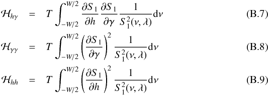 and with:
 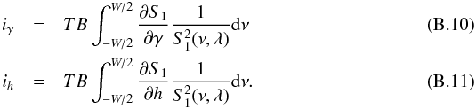 Since
Since  by construction of the MLE solution, Eqs. (B.5) and (B.6) will provide the solution for Δh and Δγ as a function of Δb as:
 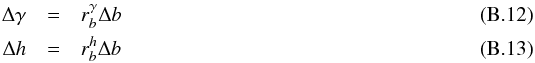 with
with 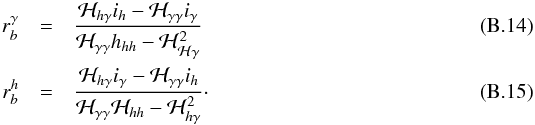 The bias on the mode amplitude
  can be expressed as
 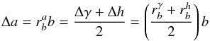 (B.16)where a = lnA. Equations (B.12) and (B.13) are the ratios for a notional bias in B. Since the calculation provided above was done assuming that the frequency window was large with respect to the mode linewidth, we must point out that the stellar background itself may be substantially over- or underestimated when the linewidth is not small compared to the window of interest. As a consequence, even though the sensitivity to the background bias may be small, it is likely that the effective biases on mode linewidth and mode height may be larger because the bias on the stellar background may be large.
Appendix B.3: Effect of a different estimated splitting and inclination angle
As shown by Toutain & Appourchaux (1994), there is no correlation between the splitting error and the mode linewidth error or the mode height error. It implicitly means that at least to first order there should not be any systematic errors in the mode linewidth and mode height measurements resulting from an incorrectly estimated splitting. We study here is the second order effect.
When the fitted spectra S1 is different from S0, we can write to the second order : 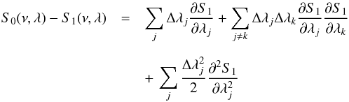 (B.17)where λj are γ,h, b and νs (where νs is the mode splitting of the multiplet). Inserting Eqs. (B.17) in (B.3) one gets:
 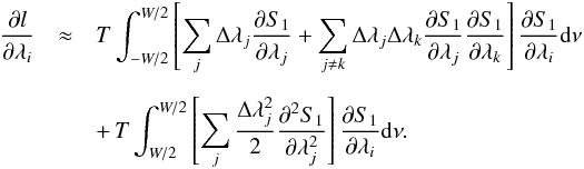 (B.18)Here we note that the parity with respect to frequency (ν) will play a key role in whether some terms disappears or not. For instance, all derivatives of S1 with respect to γ, h and b will be even in (ν − ν0), where ν0 is the central mode frequency of the multiplet. The derivatives of S1 with respect to ν0 are odd in (ν − ν0) while the derivative of S1 with respect to νs is even in (ν − ν0). Therefore of all the cross terms involving γ,h,b, and ν0 are null. At first sight all of the cross terms with νs would not necessarily be null. But since the multiplet is composed of a superposition of several peaks, there is a local parity in the function around the mode frequency νlm, i.e. around (ν − νlm) which Toutain & Appourchaux (1994) termed as locally odd (or even) function, in other words:
 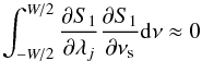 (B.19)with λj ≠ νs. We can then rewrite Eq. (B.18) for the splitting νs as
 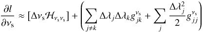 (B.20)\pagebreak
and then for γ,h and b (=λi′) as: 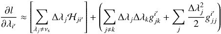 (B.21)where
  is written as:
 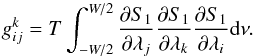 (B.22)The terms in brackets in Eqs. (B.20) and (B.21) represent the first order terms, while the terms in parentheses are the higher order terms. Since by construction of the MLE solution, it is clear that the solution to the system of equation is non-linear. As a consequence, the systematic errors on mode linewidth and mode height strongly depend to the second order to deviation to the nominal splitting.
This simple analysis shows that the derivation of the biases due to splitting is not straightforward. This is why we resorted to the single-fit approach of Toutain et al. (2005) in order to have some clues as to the magnitude of the effect of an incorrect splitting. Figures A.2 and A.3 shows the results of the numerical calculation of the systematic errors on mode linewidth, mode height, and mode amplitude biases as a function of the fitted splitting, for two different nominal splitting and mode linewidth. Figure A.4 shows the results of the numerical calculation of the systematic errors on mode linewidth, mode height, and mode amplitude biases as a function of the fitted inclination angle, for a single nominal splitting and mode linewidth, and for two nominal inclination angles.
Appendix B.4: Effect of different assumption on mode height ratio
Here we assume that the fitted mode profile is given by a superposition of a profile for each l such that we can write 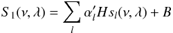 (B.23)where
  is the fixed (or fitted) mode height ratio normalised to the l = 0 degree, i.e.
  . We have a similar expression for the reference profile S0 introducing the mode height H and the mode height ratio αl. Therefore we can write that:
 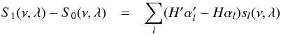 (B.24)Using Eq. (B.3) we can write for the fitted mode height:
 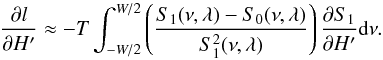 (B.25)Deriving Eq. (B.23) with respect to H′, we have:
 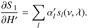 (B.26)Since
  , using Eqs. (B.24), (B.25) and (B.26) we can derive that we have:
  (B.27)\newpagewith
 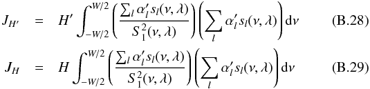 assuming that the cross terms between different l are negligible, Eqs. (B.28) and (B.29) can be approximated as:
 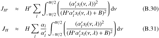 both equations can be simplified as
 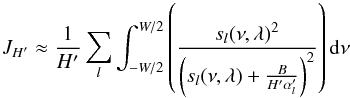 (B.32)and
 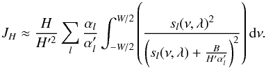 (B.33)We can calculate these integrals using Eq. (A1) of Toutain & Appourchaux (1994) by replacing β by β′/α′, where β′ = B/H′ and assuming that the frequency window is large compared to the linewidth. Omitting the common factors, we finally obtain:
 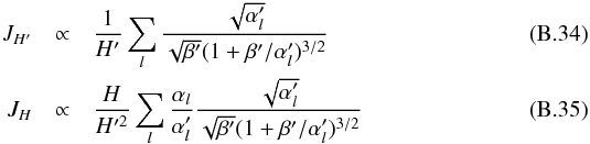 then using Eq. (B.27), we have:
  (B.36)Then to first order in ΔH = H′ − H and in
  , we can write
  (B.37)such that we have the following approximation:
  (B.38)
 |
Fig. B.1
Corrected mode linewidth, mode height, and mode amplitude (top), and relative values of these parameters with respect to the reference fit (bottom) as a function of mode frequency for KIC 1435467. The grey band indicates the range of systematic error around the reference fit values of ±15% for mode linewidth and mode height, of ±5% for mode amplitude. The error bars are those of the reference fit. |
| Open with DEXTER | |
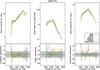 |
Fig. B.2
Corrected mode linewidth, mode height, and mode amplitude (top), and relative values of these parameters with respect to the reference fit (bottom) as a function of mode frequency for KIC 2837475. The grey band indicates the range of systematic error around the reference fit values of ±15% for mode linewidth and mode height, of ±5% for mode amplitude. The error bars are those of the reference fit. |
| Open with DEXTER | |
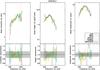 |
Fig. B.3
Corrected mode linewidth, mode height, and mode amplitude (top), and relative values of these parameters with respect to the reference fit (bottom) as a function of mode frequency for KIC 3424541. The grey band indicates the range of systematic error around the reference fit values of ±15% for mode linewidth and mode height, of ±5% for mode amplitude. The error bars are those of the reference fit. |
| Open with DEXTER | |
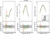 |
Fig. B.4
Corrected mode linewidth, mode height, and mode amplitude (top), and relative values of these parameters with respect to the reference fit (bottom) as a function of mode frequency for KIC 6116048. The grey band indicates the range of systematic error around the reference fit values of ±15% for mode linewidth and mode height, of ±5% for mode amplitude. The error bars are those of the reference fit. |
| Open with DEXTER | |
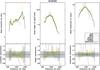 |
Fig. B.5
Corrected mode linewidth, mode height, and mode amplitude (top), and relative values of these parameters with respect to the reference fit (bottom) as a function of mode frequency for KIC 6508366. The grey band indicates the range of systematic error around the reference fit values of ±15% for mode linewidth and mode height, of ±5% for mode amplitude. The error bars are those of the reference fit. |
| Open with DEXTER | |
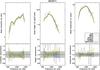 |
Fig. B.6
Corrected mode linewidth, mode height, and mode amplitude (top), and relative values of these parameters with respect to the reference fit (bottom) as a function of mode frequency for KIC 6679371. The grey band indicates the range of systematic error around the reference fit values of ±15% for mode linewidth and mode height, of ±5% for mode amplitude. The error bars are those of the reference fit. |
| Open with DEXTER | |
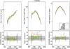 |
Fig. B.7
Corrected mode linewidth, mode height, and mode amplitude (top), and relative values of these parameters with respect to the reference fit (bottom) as a function of mode frequency for KIC 7103006. The grey band indicates the range of systematic error around the reference fit values of ±15% for mode linewidth and mode height, of ±5% for mode amplitude. The error bars are those of the reference fit. |
| Open with DEXTER | |
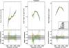 |
Fig. B.8
Corrected mode linewidth, mode height, and mode amplitude (top), and relative values of these parameters with respect to the reference fit (bottom) as a function of mode frequency for KIC 7206837. The grey band indicates the range of systematic error around the reference fit values of ±15% for mode linewidth and mode height, of ±5% for mode amplitude. The error bars are those of the reference fit. |
| Open with DEXTER | |
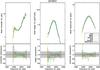 |
Fig. B.9
Corrected mode linewidth, mode height, and mode amplitude (top), and relative values of these parameters with respect to the reference fit (bottom) as a function of mode frequency for KIC 8379927. The grey band indicates the range of systematic error around the reference fit values of ±15% for mode linewidth and mode height, of ±5% for mode amplitude. The error bars are those of the reference fit. |
| Open with DEXTER | |
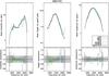 |
Fig. B.10
Corrected mode linewidth, mode height, and mode amplitude (top), and relative values of these parameters with respect to the reference fit (bottom) as a function of mode frequency for KIC 8694723. The grey band indicates the range of systematic error around the reference fit values of ±15% for mode linewidth and mode height, of ±5% for mode amplitude. The error bars are those of the reference fit. |
| Open with DEXTER | |
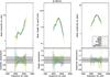 |
Fig. B.11
Corrected mode linewidth, mode height, and mode amplitude (top), and relative values of these parameters with respect to the reference fit (bottom) as a function of mode frequency for KIC 9139151. The grey band indicates the range of systematic error around the reference fit values of ±15% for mode linewidth and mode height, of ±5% for mode amplitude. The error bars are those of the reference fit. |
| Open with DEXTER | |
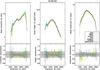 |
Fig. B.12
Corrected mode linewidth, mode height, and mode amplitude (top), and relative values of these parameters with respect to the reference fit (bottom) as a function of mode frequency for KIC 9139163. The grey band indicates the range of systematic error around the reference fit values of ±15% for mode linewidth and mode height, of ±5% for mode amplitude. The error bars are those of the reference fit. |
| Open with DEXTER | |
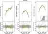 |
Fig. B.13
Corrected mode linewidth, mode height, and mode amplitude (top), and relative values of these parameters with respect to the reference fit (bottom) as a function of mode frequency for KIC 9206432. The grey band indicates the range of systematic error around the reference fit values of ±15% for mode linewidth and mode height, of ±5% for mode amplitude. The error bars are those of the reference fit. |
| Open with DEXTER | |
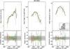 |
Fig. B.14
Corrected mode linewidth, mode height, and mode amplitude (top), and relative values of these parameters with respect to the reference fit (bottom) as a function of mode frequency for KIC 9812850. The grey band indicates the range of systematic error around the reference fit values of ±15% for mode linewidth and mode height, of ±5% for mode amplitude. The error bars are those of the reference fit. |
| Open with DEXTER | |
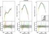 |
Fig. B.15
Corrected mode linewidth, mode height, and mode amplitude (top), and relative values of these parameters with respect to the reference fit (bottom) as a function of mode frequency for KIC 10162436. The grey band indicates the range of systematic error around the reference fit values of ±15% for mode linewidth and mode height, of ±5% for mode amplitude. The error bars are those of the reference fit. |
| Open with DEXTER | |
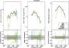 |
Fig. B.16
Corrected mode linewidth, mode height, and mode amplitude (top), and relative values of these parameters with respect to the reference fit (bottom) as a function of mode frequency for KIC 10355856. The grey band indicates the range of systematic error around the reference fit values of ±15% for mode linewidth and mode height, of ±5% for mode amplitude. The error bars are those of the reference fit. |
| Open with DEXTER | |
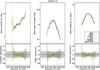 |
Fig. B.17
Corrected mode linewidth, mode height, and mode amplitude (top), and relative values of these parameters with respect to the reference fit (bottom) as a function of mode frequency for KIC 10454113. The grey band indicates the range of systematic error around the reference fit values of ±15% for mode linewidth and mode height, of ±5% for mode amplitude. The error bars are those of the reference fit. |
| Open with DEXTER | |
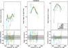 |
Fig. B.18
Corrected mode linewidth, mode height, and mode amplitude (top), and relative values of these parameters with respect to the reference fit (bottom) as a function of mode frequency for KIC 10909629. The grey band indicates the range of systematic error around the reference fit values of ±15% for mode linewidth and mode height, of ±5% for mode amplitude. The error bars are those of the reference fit. |
| Open with DEXTER | |
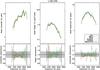 |
Fig. B.19
Corrected mode linewidth, mode height, and mode amplitude (top), and relative values of these parameters with respect to the reference fit (bottom) as a function of mode frequency for 11081729. The grey band indicates the range of systematic error around the reference fit values of ±15% for mode linewidth and mode height, of ±5% for mode amplitude. The error bars are those of the reference fit. |
| Open with DEXTER | |
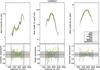 |
Fig. B.20
Corrected mode linewidth, mode height, and mode amplitude (top), and relative values of these parameters with respect to the reference fit (bottom) as a function of mode frequency for 12009504. The grey band indicates the range of systematic error around the reference fit values of ±15% for mode linewidth and mode height, of ±5% for mode amplitude. The error bars are those of the reference fit. |
| Open with DEXTER | |
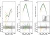 |
Fig. B.21
Corrected mode linewidth, mode height, and mode amplitude (top), and relative values of these parameters with respect to the reference fit (bottom) as a function of mode frequency for 12258514. The grey band indicates the range of systematic error around the reference fit values of ±15% for mode linewidth and mode height, of ±5% for mode amplitude. The error bars are those of the reference fit. |
| Open with DEXTER | |
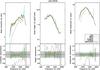 |
Fig. B.22
Corrected mode linewidth, mode height, and mode amplitude (top), and relative values of these parameters with respect to the reference fit (bottom) as a function of mode frequency for 12317678. The grey band indicates the range of systematic error around the reference fit values of ±15% for mode linewidth and mode height, of ±5% for mode amplitude. The error bars are those of the reference fit. |
| Open with DEXTER | |
© ESO, 2014
Current usage metrics show cumulative count of Article Views (full-text article views including HTML views, PDF and ePub downloads, according to the available data) and Abstracts Views on Vision4Press platform.
Data correspond to usage on the plateform after 2015. The current usage metrics is available 48-96 hours after online publication and is updated daily on week days.
Initial download of the metrics may take a while.