| Issue |
A&A
Volume 565, May 2014
|
|
|---|---|---|
| Article Number | A99 | |
| Number of page(s) | 13 | |
| Section | The Sun | |
| DOI | https://doi.org/10.1051/0004-6361/201423450 | |
| Published online | 19 May 2014 | |
Mean shape of interplanetary shocks deduced from in situ observations and its relation with interplanetary CMEs
1
Department of MathematicsUniversity of Dundee,
Dundee
DD1 4HN,
UK
e-mail:
This email address is being protected from spambots. You need JavaScript enabled to view it.
2
Observatoire de Paris, LESIA, UMR 8109 (CNRS),
92195
Meudon Principal Cedex,
France
e-mail:
This email address is being protected from spambots. You need JavaScript enabled to view it.
3
Instituto de Astronomía y Física del Espacio, UBA-CONICET,
CC. 67, Suc.
28, 1428
Buenos Aires,
Argentina
e-mail:
This email address is being protected from spambots. You need JavaScript enabled to view it.
4
Departamento de Física, Facultad de Ciencias Exactas y Naturales,
Universidad de Buenos Aires, 1428
Buenos Aires,
Argentina
e-mail:
This email address is being protected from spambots. You need JavaScript enabled to view it.
5
Departamento de Ciencias de la Atmósfera y los Océanos, Facultad
de Ciencias Exactas y Naturales, Universidad de Buenos Aires,
1428
Buenos Aires,
Argentina
e-mail:
This email address is being protected from spambots. You need JavaScript enabled to view it.
Received:
17
January
2014
Accepted:
18
March
2014
Abstract
Context. Shocks are frequently detected by spacecraft in the interplanetary space. However, the in situ data of a shock do not provide direct information on its overall properties even when a following interplanetary coronal mass ejection (ICME) is detected.
Aims. The main aim of this study is to constrain the general shape of ICME shocks with a statistical study of shock orientations.
Methods. We first associated a set of shocks detected near Earth over 10 years with a sample of ICMEs over the same period. We then analyzed the correlations between shock and ICME parameters and studied the statistical distributions of the local shock normal orientation. Supposing that shocks are uniformly detected all over their surface projected on the 1 AU sphere, we compared the shock normal distribution with synthetic distributions derived from an analytical shock shape model. Inversely, we derived a direct method to compute the typical general shape of ICME shocks by integrating observed distributions of the shock normal.
Results. We found very similar properties between shocks with and without an in situ detected ICME, so that most of the shocks detected at 1 AU are ICME-driven even when no ICME is detected. The statistical orientation of shock normals is compatible with a mean shape having a rotation symmetry around the Sun-apex line. The analytically modeled shape captures the main characteristics of the observed shock normal distribution. Next, by directly integrating the observed distribution, we derived the mean shock shape, which is found to be comparable for shocks with and without a detected ICME and weakly affected by the limited statistics of the observed distribution. We finally found a close correspondence between this statistical result and the leading edge of the ICME sheath that is observed with STEREO imagers.
Conclusions. We have derived a mean shock shape that only depends on one free parameter. This mean shape can be used in various contexts, such as studies for high-energy particles or space weather forecasts.
Key words: Sun: coronal mass ejections (CMEs) / Sun: heliosphere / magnetic fields / solar-terrestrial relations
© ESO, 2014
1. Introduction
Interplanetary shocks are formed when a solar wind disturbance propagates significantly faster than the surrounding medium (typically above the local fast MHD mode speed). Shocks in the inner heliosphere are generally weak, as the fast-mode MHD Mach number is typically between 1 and 2 (Volkmer & Neubauer 1985). They are also less frequent than at larger solar distance. Their occurrence frequency peaks in the range 2−5 AU and decreases at larger distances, as reviewed by Neugebauer (2013). There is also a strong correlation between the shock frequency and the solar cycle.
Interplanetary shocks have two main origins. First, a shock can originate in a fast solar wind stream with a typical speed above 600 km s-1, which overtakes a slower stream with a speed around 400 km s-1 (e.g., see the reviews of Balogh et al. 1999; Smith 2008). The interaction strengthens with solar distance and forms a stream interaction region (SIR) that is edged by a forward and a backward shock. At 1 AU, Jian et al. (2006) have found that only 24% of SIRs have shocks. These shocks are still in a phase of building up at 1 AU, and the shocks are small and transient structures, as observed with multi spacecraft (Jian et al. 2009). The sources of fast streams are typically large and stable coronal holes. They, therefore, build more stable interacting regions, which then rotate with the Sun and are called corotating interaction regions (CIRs), and are present, especially, at large latitudes (see the reviews of Gosling & Pizzo 1999; Balogh & Jokipii 2009).
A second source of shocks is transient in nature and is associated with coronal mass ejections (CMEs). These are detected in situ by their enhanced magnetic field strength and are correlated with a broad set of plasma signatures, including a lower proton temperature and/or enhanced abundances of some minority ions (see Richardson & Cane 2010, and references therein). When detected in situ, they are called interplanetary CMEs (ICMEs). These ejecta are formed by plasma and magnetic field ejected during a solar eruption. The front part of ICMEs is typically faster than the encountered solar wind, so ICMEs are typically preceded by a sheath of compressed plasma and magnetic field. Therefore, in the following, we distinguish the ICMEs from the sheath and their associated shocks. Magnetic clouds (MCs) are a subset of ICMEs with an enhanced magnetic field strength, a smooth rotation of the magnetic field direction through a large angle, and a low proton temperature compared to the expected one in the solar wind (see the reviews of Gosling et al. 1995; Dasso et al. 2005).
Sheeley et al. (1985) found that at least 72% (49/68) of the shocks observed in situ by Helios 1 spacecraft were associated with CMEs observed with a coronagraph. Only 2% of the observed shocks lacked an associated CME. Lindsay et al. (1994) confirmed this by finding that at least 80% (36/45) of shocks at 0.7 AU are associated with a CME. At 1 AU and with in situ data, Berdichevsky et al. (2000) found that only 43% (18/42) of shocks are associated to ICMEs during a solar minimum period (1994−1997). Analyzing seven years of data with Wind and ACE, Oh et al. (2007) found that 79% (196/246) of shocks are associated to ICMEs (MCs and ejecta), while 21% (40/246) of shocks are associated to CIRs (or high speed streams, HSS). Moreover, the shock frequency has a cycle dependence closely related with the yearly mean sunspot number (see Fig. 2 of Oh et al. 2007). A very similar frequency dependence is found for ICMEs (Robbrecht et al. 2009; Boursier et al. 2009). The above results were confirmed and extended by Lai et al. (2012), who found that shocks associated to CIRs have a nearly constant frequency during the solar cycle and are only as numerous as ICME shocks during solar minimum, while ICME shocks are much more numerous at other times (their Fig. 3). This tendency is stronger in the inner heliosphere (their Fig. 4) and is not present with STEREO data, as the data are provided only at 1 AU and during a deep solar minimum.
Interplanetary structures can affect the transport of energetic particles in the heliosphere (e.g., Masson et al. 2012,and references therein). The presence of interplanetary shocks is typically associated with a transient variation of energetic particles abundances. On the one hand, acceleration at an interplanetary shock driven by ICMEs is one of the most possible mechanisms involved in the production of gradual energetic particle events (e.g., Vainio 2009). On the other hand, flux decrease of energetic particles over a very large range of energies is also associated with ICMEs and ICME-shocks. At lower energies, this effect is observed in situ in the solar wind by spacecraft, while at higher energies (cosmic rays) it is observed at ground level by neutron monitors (e.g., Simpson 1954) or by water Cherenkov radiation detectors (e.g., Dasso et al. 2012).
A classical two-step Forbush decrease (FD) of energetic particles is typically observed in agreement with the passage of an ICME and its driven shock. The seminal ideas of a two-step FD were presented by Barnden (1973a,b). Now, it is believed that the first step (i.e., the first decrease in the energetic particles flux) is produced by a diffusive barrier associated with the turbulent region behind the shock (i.e., the sheath). The decrease starts in agreement with the arrival of the shock and typically continues during many days with a very slow recovery, which is determined largely by the shock properties (Cane et al. 1994). Thus, the effect associated with the first step (shock-step) is nonlocal and strongly linked with the open problem of the global shape of the interplanetary shocks. Instead, the second step is associated with the shock-driver itself (i.e., the ICME). This second decrease starts just when the in situ observer enters inside the ICME and finishes when the observer leaves it. Thus, the effect associated with the second step (ICME-step) is local, and more linked with the connectivity of magnetic field lines inside ICMEs. A typical two-step FD can be seen in Fig. 1 of Cane (2000).
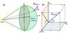 |
Fig. 1 Geometry of a shock propagating from the Sun and related-orientation parameters in
the heliocentric coordinates: a) the shock surface and the normal vector
|
However, recent statistical results presented by Jordan et al. (2011) have shown that only 80 created FDs, and only 13 created the expected two-step FDs among 233 ICMEs that should have created two-step FDs. Advances in the knowledge of the general geometrical shape of interplanetary shocks driven by ICMEs (and also on the specific diffusive properties in the sheath region) will help to clarify these controversial results. As such, they will also help to determine when two-step FDs can be expected and to answer other open questions on the effects of shocks on cosmic rays.
In the majority of cases, interplanetary shocks are crossed only by one spacecraft. As such, the in situ data derived from the analysis of the shock properties are only local and conclusions from single observations are therefore limited. However, because the twin spacecraft of the Helios mission were in the ecliptic plane and always closer or much less than 130° in longitude, a relatively large number of ICME shocks were detected at both spacecraft. Adding data from IMP-8 spacecraft, de Lucas et al. (2011) analyzed 132 shocks observed by a pair of spacecraft. They found that the probability to detect the same shock at both spacecraft decreases roughly linearly with the longitudinal separation of spacecraft, with a probability of 0.5 for a longitudinal separation of 90°. This provides an implicit constraint on the mean longitudinal extension of ICME shocks. Next, a limited sample of ICMEs have been analyzed by the STEREO twin spacecraft associated to other spacecraft, such as ACE, MESSENGER, VEX, or Wind (Kilpua et al. 2011; Farrugia et al. 2011; Möstl et al. 2012). These studies provide constraints on the spatial extension and geometry of shocks in specific events. So far, the largest number of spacecraft crossings remains the event of January 1978 with five spacecraft crossings. Burlaga et al. (1981) deduced a general shape for the shock and the MC axis, which are still the expected typical shapes nowadays (Möstl et al. 2012; Janvier et al. 2013). Berdichevsky et al. (2009) re-analyzed the same event and concluded that there was a strong speed gradient in longitude with a stronger speed around the apex than on the flanks of the shock. However, we would need many more observed cases with multiple spacecraft to better quantify the properties along the shock surface and its shape. This data will not be available before at least many years, so we propose and develop a statistical method below.
The main aim of this study is complementary to the previous article (Janvier et al. 2013), where we deduced the mean shape of the magnetic cloud axis at 1 AU from the probability distribution function of the local axis orientation by using a sample that contains more than 100 MCs (detected on the ecliptic plane), which is combined with geometrical considerations. In the present paper, we determine the mean shape of the shock surface in front of in situ-detected ICMEs at 1 AU on the ecliptic plane and also analyze the shock properties as a function of their distance to the shock apex. In Sect. 2, we first summarize the observations used and define the main new variables. Then, we find associated pairs of observed ICMEs and shocks. We then look into the details of the statistics of the shock properties. In particular, we look at the ICME properties for ICME-associated shocks. We also compare sets of shocks associated with ICMEs with sets of shocks with no in situ-detected ICMEs. In Sect. 3, we derive an analytical model of the shock front, aiming at interpreting the main results of Sect. 2 with the simplest model possible. In Sect. 4, we do the reverse procedure, which is to derive a method that allows the computation of the mean shock shape from the observed distribution of shock normals. In Sect. 4.3, we finally show that this derived mean shape is close to the front shape of an ICME observed by STEREO-A imagers. Finally, in Sect. 5, we summarize our results, conclude, and outline potential applications.
2. Observations
2.1. Set of observed shocks
In the present paper, we use the list of shocks studied in Wang et al. (2010) in the continuity of the work of Wang et al. (2009). This list consists of shock events that have been detected by the ACE spacecraft, which is located in the solar wind, on the ecliptic plane at 1 AU from the Sun. All the shock parameters have been calculated using a shock-fitting procedure for the MHD Rankine-Hugoniot relations as presented in Lin et al. (2006). The list extends from February 1998 to August 2008, and the authors have reported a total of 286 events. Among them, 257 events are identified as shocks, while the remaining 29 events are identified with shock-like structures.
The list given in Wang et al. (2010) reports on
different parameters: the local orientation of the shock normal vector
 , the speed normal
to the shock Vsn in the rest frame (as used for ACE
data), the ratio of the downstream density over the upstream density ρ2/ρ1,
and the fast-mode Mach numbers in the upstream and downstream regions Mf1,Mf2.
, the speed normal
to the shock Vsn in the rest frame (as used for ACE
data), the ratio of the downstream density over the upstream density ρ2/ρ1,
and the fast-mode Mach numbers in the upstream and downstream regions Mf1,Mf2.
Analyzing the distribution of the shock parameters for both the shock and shock-like events, we found no interesting properties for the shock-like events, probably due to the small portion of events (29 events out of the 286 detected by ACE). Indeed, the distributions are more scattered for all four parameters (ρ2/ρ1,Vsn,Mf1,Mf2) than for the shocks with no clear tendency. Therefore, in the following, we only study the shocks, since the nature of the shock-like events is dubious.
2.2. Angles defining the shock normal
The geocentric solar ecliptic (GSE) system of reference (with unit vectors
 ,
,
 ,
,
 ) is defined such
that points from the
Earth toward the Sun, is in the ecliptic
plane and in the direction opposite to the planetary motion, and
points to the north
pole.
) is defined such
that points from the
Earth toward the Sun, is in the ecliptic
plane and in the direction opposite to the planetary motion, and
points to the north
pole.
The direction of a shock is classically defined by its normal vector
(Fig. 1a) given by three coordinates nx, ny, and nz in the GSE system of
reference (Fig. 1b). Projecting
on a plane
perpendicular to , we introduce the
angle i to
quantify the inclination between this projected vector
 and the direction (Fig. 1b). The value i = 0° corresponds to a normal vector in
the ecliptic plane, and i ranges from −180° to 180° with 90° and −90° corresponding to north or
south orientations.
and the direction (Fig. 1b). The value i = 0° corresponds to a normal vector in
the ecliptic plane, and i ranges from −180° to 180° with 90° and −90° corresponding to north or
south orientations.
We also define the angle between the direction  and
. This angle is
named the location angle λ (similarly as in Janvier et al. 2013) as it informs on the relative location of the spacecraft
crossing the shock structure from the apex. It quantifies the departure from the radial
direction: if λ =
0°, it means that the spacecraft crosses the shock right
along its apex. A deviation from λ = 0° indicates that the structure is
crossed at any point on a circle surrounding the apex. The larger the value of
λ is (up to
90°), the further
the spacecraft is from the apex. However, λ does not indicate the exact location on the shock
since that would require knowing the structure of the shock surface.
and
. This angle is
named the location angle λ (similarly as in Janvier et al. 2013) as it informs on the relative location of the spacecraft
crossing the shock structure from the apex. It quantifies the departure from the radial
direction: if λ =
0°, it means that the spacecraft crosses the shock right
along its apex. A deviation from λ = 0° indicates that the structure is
crossed at any point on a circle surrounding the apex. The larger the value of
λ is (up to
90°), the further
the spacecraft is from the apex. However, λ does not indicate the exact location on the shock
since that would require knowing the structure of the shock surface.
As such, (λ,i) defines the spherical coordinates where
is the polar axis.
Then, both angles λ and i can directly be related with the more standard
angles θ and
φ, which
are the latitude and the longitude of as given in GSE:
 This
definition considers that λ > 0 for shocks propagating
away from the Sun. For this case and since sinθ = sinisinλ,
i has the
same sign as the latitude θ. Reverse shocks traveling toward the Sun (e.g.,
shocks produced in the rear of ICMEs, which are in strong expansion) correspond to
λ<
0. They are not considered in the present work but can be considered
using this mathematical convention in future studies.
This
definition considers that λ > 0 for shocks propagating
away from the Sun. For this case and since sinθ = sinisinλ,
i has the
same sign as the latitude θ. Reverse shocks traveling toward the Sun (e.g.,
shocks produced in the rear of ICMEs, which are in strong expansion) correspond to
λ<
0. They are not considered in the present work but can be considered
using this mathematical convention in future studies.
In Fig. 2a, we look at the distribution of the inclination angle i for the 257 shocks detected by ACE with 24 bins. The distribution is scattered along the values of i, and apart a higher concentration of events for i > 0 values, there is no global tendency. We also computed the distribution of |i| − 90° (not presented here), where ||i|−90°| ~ 90° refers to a shock normal that is E/W-orientated, and ||i|−90°| ~ 0° to a shock normal that is N/S orientated. We found no evidence of a preferred orientation.
For small λ
values, a perturbation to typically induces
a large variation of i; then a uniform distribution of i could be expected for
small λ
values. To avoid such an effect, we present the distribution of i for the same bins but
with a selection parameter, 30° ≤
λ ≤ 90°, in Fig. 2b. Removing small values of λ therefore insures more robust results. This new
distribution seems more uniform than in Fig. 2a,
although the same tendency for positive values of i remains. Again, by
separating E/W or N/S orientated shocks with this selection, we found no significant
tendencies.
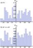 |
Fig. 2 a) Distribution of the inclination angle i (see Fig. 1b) for shocks detected by ACE and for 24 bins. b) i distribution for the same set of shocks with a selection on λ as: 30° ≤ λ ≤ 90°. |
We interpret the above results as follows. During the ten years of the data set, the Sun
launched CMEs (i.e., shock drivers) from any longitude and from a broad range of
latitudes. This implies that the spacecraft crossed the shocks with a uniform probability.
Then, the above results of nearly uniform distributions of i and ||i|−900|
indicate that there is no privileged direction of around the
Sun-apex line.
These results seem at first surprising, since 3D numerical simulations show that an ICME and its front shock can be significantly deformed during their propagation. Indeed, these deformations are seen within simulations that initialize a CME with a flux rope, which is out of equilibrium in the corona (e.g. Manchester et al. 2008; Taubenschuss et al. 2010), and are seen even more in simulations that initialize a CME within the solar wind with a pressure pulse, since there is no intrinsic CME magnetic field to insure an internal coherence (e.g., Lee et al. 2013; Xie et al. 2013). However, the characteristics of the deformation depend on many parameters, including the geometry of the interaction, the relative orientation in particular, and strength of the magnetic field within the flux-rope and the solar wind. As such, the deformations are strongly case-dependent (see Lugaz & Roussev 2011 for a review). For example, an ICME is deformed to a concave-outward shape if the ICME is traveling in a slow wind, and edged on both sides by fast winds (Manchester et al. 2004; Taubenschuss et al. 2010). These deformations are therefore only present with specific conditions, such as a very dense slow solar wind and an ICME that is broad enough to be significantly affected by the fast winds on both sides. Indeed, this concave-outward shape is not present in many 3D-MHD simulations and is rarely observed by STEREO imagers (Lugaz & Roussev 2011). To conclude, significant deformations of ICMEs and their shocks are strongly case-dependent.
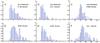 |
Fig. 3 Distributions of a) the ratio of the downstream density over the upstream density ρ2/ρ1, b) the upstream fast-mode Mach number Mf1, and c) the shock speed Vsn for fICME = − 1, which has no associated ICME in situ detected. Distributions of d) ρ2/ρ1, e) Mf1, and f) Vsn for all shocks related with an in situ detected ICME (fICME = 0,1or2). |
In light of the results obtained from numerical simulations of propagating ICMEs and shocks, we can interpret the nearly uniform distributions of i as a consequence of the statistical analysis, which only retains the features common to a majority of events, and therefore smoothes the specific properties of each event. Then, we conclude that we do not detect a global trend on i within the limit of the finite statistics used. Finally, these results are compatible with a mean shock shape having a rotation symmetry around the Sun-apex direction.
2.3. Association with ICMEs
Before doing a further analysis of the shock properties, we search for an association of these shocks with observed ICMEs, since shock properties could depend on the type of the associated driver. To do so, we relate shocks with the propagation of ICMEs under the condition that both events can be strongly correlated. The list of Wang et al. (2010) provides the time at which ACE detected the shocks. Then, we can correlate them with ICMEs occurring during the same range of time.
To associate a shock event to an ICME event, we took the list of Richardson & Cane (2010) who report on 317 ICMEs observed from 1996 to 2009. A time is given for the beginning of the disturbance (tdist), which can be associated with a shock time (tshock). The times for the start and the end of each detected ICME are also listed (tstart and tend). The time difference tstart − tdist defines the sheath of the ICME.
The list of ICMEs (Table 1 of Richardson & Cane 2010) provides a complete set of parameters, such as the difference of ICME speeds between the front and the rear (ΔV), the mean speed of the ICME (⟨ V ⟩), the mean value of the magnetic field (⟨ B ⟩), and the geomagnetic effectivity measured by the Dst index. The Dst index used is the minimum value of Dst for the geomagnetic storm that associated with the passage of the ICME/shock. The list also provides a flag, depending on whether a magnetic structure was detected inside them. In case a magnetic cloud (MC) was detected, a flag 2 was given to the ICME event. MC-like events were given a flag 1, and no MC cases have a flag 0.
We followed simple rules for the association of ICMEs and shocks. First, we associate each ICME with the closest shock from Wang’s list by comparing the event time of the shock and tdist. This step leads to the definition of only one potential shock per ICME. Then all shocks are set with a flag fICME = −1. For each shock, we scan the ICME list and associate the ICME that has the closest disturbance time to the shock time, which verifies that this shock is the closest from tdist (first step). We select an interval of 2 h (| tdist − tshock| < 2 h), so to only keep ICME disturbances and shocks that occur almost simultaneously. The flag fICME for those shocks is then changed to 0, 1, or 2, which is similar to the ICME flag. We find 36 cases of shocks without MC, 36 cases of shocks associated with MC-like, and 45 shocks associated with MCs.
Finally, shocks that occur during an ICME (tdist + 2 h < tshock < tend), or outside an ICME but within 6 h of the ICME end (tend < tshock < tend + 6 h) are removed from the list. This last step is necessary, since we want to analyze the shocks in front of ICMEs that are not perturbed by the presence of a previous ICME. However, it is worth noting that our ICME-shock technique does not fully ensure that there are no interactions between two ICMEs since measurements are local. Moreover, taking 6 h after the end of the ICME is arbitrary. However, we also considered a more stringent condition for which all shocks corresponding to tshock − tend < 48 h were removed. The same analysis, as done in Sect. 2.4, showed no difference, and the value of Δt = 6 h was kept, since more cases can then be considered. The remaining 99 cases are shocks for which fICME is still −1 and correspond to shocks that are not correlated with the data coming from the spacecraft that locally crosses an ICME. This does not mean that there is no associated ICME, but the possibly related ICME has not crossed the spacecraft during the shock crossing. Another possible explanation could be that these shocks are created by a fast stream overtaking a slow one.
2.4. Statistical analysis of shock properties
In the following, we look at the shock property distributions after their possible association with ICMEs. In Fig. 3, we present the distributions of the density ratio ρ2/ρ1, the upstream fast-mode Mach number Mf1, and the shock normal speed Vsn for all shocks that are not associated to an ICME (no ICME was detected in situ, hence fICME = −1; Figs. 3a,b,c) and the same distributions for shocks associated with ICMEs (fICME = 0 to 2; Figs. 3d,e,f). We found similar distributions for shocks separated into categories fICME = 0, fICME = 1, fICME = 2, but the statistical fluctuations are larger since the number of cases is rather small (~40) for each category. We therefore show in situ-detected ICME shocks altogether.
The distribution for ρ2/ρ1 only starts at ρ2/ρ1> 1, which verifies the properties of the shocks since the downstream density (ρ2) is higher than the upstream density (ρ1). Both distributions for non-detected ICME shocks and ICME shocks are non-uniform with an abrupt increase to the peak and a tail extending toward ρ2/ρ1 ~ 5. However, note that the peaks are different for the two distributions with a peak at ρ2/ρ1 ~ 1.5 (and a median for the distribution of 2) for the non-detected ICME shocks and ρ2/ρ1 ~ 2 (and a median for the distribution of 2.2) for ICME shocks. This indicates that shocks related with ICMEs are stronger than those non-ICME associated. This is an expected result as shock strength typically decreases with distance to the apex, so that shocks without a detected ICME behind, away from the apex, are expected to be weaker.
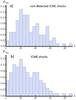 |
Fig. 4 a) Distribution of the location angle λ (see Fig. 1) for fICME = −1, which has no associated ICME in situ detected. The distribution is given for a bin size Δλ = 4.5°. b) Distribution of λ with same bins for all shocks related with ICMEs (fICME = 0,1 or 2). |
The distributions for the upstream fast-mode Mach number, Mf1, are similar, and both distributions tend to peak around the same values around ~1.5, as shown in Figs. 3b,e. Note however that there are less cases with higher Mf1 for non-detected ICME shocks; its median is equal to 1.7 for non-detected ICME shocks and equal to 2.03 for the ICME shocks cases. This, again, indicates that ICME shocks tend to be stronger than non-detected ICME shocks.
The distributions of the shock speed, Vsn (Figs. 3c,f), are almost Gaussian-like with different peaks and broadening. The peak of the distribution is around Vsn ~ 400 km s-1 (median equal to 433 km s-1) for non-detected ICME shocks, while it is ~450 km s-1 (median equal to 517 km s-1) for ICME-shocks, which indicates that shocks associated with ICMEs are faster. The wide broadening of the ICME-shocks distribution indicates a wide range of speeds (with a maximum value at Vsn = 1000 km s-1), while the speed of non-detected ICME shocks is more concentrated around the peak value. Despite these differences, the striking evidence of similar distributions indicates that non-detected ICME shocks and ICME-shocks may have a similar nature.
Finally, we present the distribution of the location angle λ,
 ,
by binning the total sets with Δλ = 4.5° in Fig. 4. Similar to the previous distributions, there is a strong similarity
between non-detected ICME and ICME-shocks. Both distributions start with an abrupt
increase toward the same peak value λ = 20° with a tail decreasing towards
90°. The low
numbers of shocks detected for small values of λ can be explained by the geometry of the shock
itself, as follows. Since a shock is a 2D structure (Fig. 1a), the extension of its surface near the apex (where λ → 0°) is
small. There is then less chance of crossing the shock at its apex than at other parts of
its structure (see Sect. 3). Moreover, the
difference of
near λ =
0° between Fig. 4a and
b indicates that there are even less non-ICME shocks detected near the apex.
,
by binning the total sets with Δλ = 4.5° in Fig. 4. Similar to the previous distributions, there is a strong similarity
between non-detected ICME and ICME-shocks. Both distributions start with an abrupt
increase toward the same peak value λ = 20° with a tail decreasing towards
90°. The low
numbers of shocks detected for small values of λ can be explained by the geometry of the shock
itself, as follows. Since a shock is a 2D structure (Fig. 1a), the extension of its surface near the apex (where λ → 0°) is
small. There is then less chance of crossing the shock at its apex than at other parts of
its structure (see Sect. 3). Moreover, the
difference of
near λ =
0° between Fig. 4a and
b indicates that there are even less non-ICME shocks detected near the apex.
The distribution of λ, which is non uniform, is an interesting property to analyze, since the location angle is directly related with the 2D structure of the shock surface (Fig. 1a). However, all shocks do not have the same properties (different ρ2/ρ1,Mf1, ...), and using the whole sets of shocks to infer a general structure can be misleading. Therefore, in the following, we study the correlations between λ and other shock parameters in details.
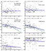 |
Fig. 5 Top: correlation between λ and ρ2/ρ1 for a) non-detected ICME shocks (fICME = − 1) and b) shocks associated with ICMEs (fICME = 0,1 and 2). The correlation is very weak for both cases. Middle: correlation between λ and the shock speed Vsn for c) non-detected ICME shocks and d) shocks associated with ICMEs. The correlation between the two parameters is very large, and the same tendency is found for different types of shocks. This tendency is compatible with Vsn∝ cosλ (green dashed lines). Bottom: e) correlation between λ and the ICME ΔV (difference between the front and the rear velocities), and f) correlation between λ and Dst for shocks with ICMEs. |
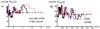 |
Fig. 6 Median of |
2.5. Correlations
In Fig. 5, we present the correlations between λ and several selected parameters to show possible tendencies. The correlation with ρ2/ρ1 is shown in Figs. 5a and b for non-detected ICME shocks and ICME-shocks. Both Pearson and Spearman coefficients (cp and cs) are given with the fitting function of the correlations. Similarly to all other shock characteristics except Vsn, we find no significant correlation between any shock parameters and λ for both non-ICME and ICME-shocks with both | cp | and | cs | less than 0.1.
In contrast, there is a strong correlation between Vsn and λ, as is illustrated in Figs. 5c,d. Indeed, shocks detected at and around their apex (λ < 20°) correspond to fast propagating shocks, while shocks detected far away from the apex are slower shocks. For both set of shocks, we find similar Pearson and Spearman correlation coefficients. The origin of this correlation can be understood from the properties and the geometry of ICME shocks, as follows. As a first simple approach, we consider a shock surface with a rotation symmetry around the Sun-apex direction, as represented in Fig. 7. The shock speed Vsn (normal to the shock front) is related to its local radial velocity Vρ away from the Sun, by Vsn = Vρcosλ. In the case of a self-similar expansion of the ICME from the Sun, which propagates in an unstructured solar wind, the outward velocity at any location of the expanding structure is expected to be radial. In this simplified case, we then expect a simple cosλ-dependence of Vsn. However, more generally, the shock velocity is both a function of the relative velocity between the ICME and the upstream solar wind, as well as a function of the expansion speed of the ICME. These are respectively at the origin of the propagation and the expansion sheaths (Siscoe & Odstrcil 2008). In general, this implies that Vρ is also dependent of λ, although a model derivation for Vρ(λ) is out the scope of the present study. The cosine dependence alone is shown in Fig. 5c,d with a green dashed line, which shows the main tendency of the data. This also indicates that Vρ is nearly non-dependent on λ within the data limits, where shocks with a range of apex velocities are mixed. Although not shown here, we also found no correlation between Vsn/ cosλ and λ. We conclude that the Vsn(λ) correlation found in Fig. 5c,d is mostly a geometrical effect within the limits of the event variability.
We also look at the correlation between λ and the properties of the ICMEs that are associated with the shocks (fICME = 0 to 2). We found no evident correlation, since the correlation coefficients are small, except for two parameters: ΔV and Dst index, as shown in Figs. 5e,f. The shocks detected near the apex generally have larger ΔV in the associated ICME. Indeed, when a shock is crossed at its apex, a longer distance is crossed in the ICME, which leads to a larger ΔV (see Gulisano et al. 2012). Next, the Dst index increases for shocks crossed at the apex (Fig. 5f). This index measures the geoeffectiveness of an event by monitoring the magnetic storm level in the Earth magnetosphere. The Dst index is more negative for a stronger storm. Therefore, there is a global trend of finding less geoeffective shocks associated with ICMEs when they are crossed near the apex than when they are crossed away from the apex. However, the strongest geoeffective shocks are still present for λ< 60°. Therefore, we find no clear tendency of the Dst index evolution with the location along the shock structure. Previous studies have shown that the Dst index is dominantly controlled by the amplitude and the duration of the southward magnetic field component (e.g., see the reviewed of Lavraud & Rouillard 2014). The present study, which considers a mixed sample of cases having a southward and northward magnetic field component, shows that the location of interaction between the magnetosphere and the encountered ICME (identified with λ) has indeed a much weaker effect.
2.6. Can we study all shocks altogether?
The previous correlation analysis showed no tendency. This implies that either the set of
analyzed shocks is formed by groups of events with similar characteristics, or that the
shock shape, via λ, does not depend on any parameter. Still, is it
meaningful to analyze
deduced from a selection, containing all the shocks (simply separating the non-detected
from the detected ICME shocks). Here, we further analyze the possible dependence of the
distribution
on the shock parameters with a more complex but more complete method. The aim is to
analyze whether the main
characteristics (i.e., its first moments) are a function of some parameter when the data
sample is divided in sub-groups.
To define sub-groups, we first order all the shocks as a function of one shock parameter,
for example, by increasing values of ρ2/ρ1.
We then take the first ten ordered shocks, and we compute the mean, median, and standard
deviation of the obtained histogram for λ. Then, we shift the studied set by one case to
larger ρ2/ρ1
values (removing the lowest ρ2/ρ1
value and adding the next larger one). At each creation of new sets of ten shocks with
increasing values of ρ2/ρ1,
we report the mean, median, and standard deviation of λ for each obtained
histogram. The values of the median are reported in Fig. 6 for (a) all the non-detected ICME shocks and (b) the ICME-shocks. We found no
specific evolution between the median of
and increasing ρ2/ρ1
values. The same conclusion was also found for the mean and standard deviation (not
shown).
We performed a similar analysis for the other parameters and found no further dependence
(except for Vsn and ΔV, as expected from Fig.
5c−e). These results mean that the main characteristics of
,
which are its first moments, are independent of the shock and ICME parameters, so that we
can analyze the whole set of detected ICME shocks together and, similarly, for the
non-detected ICME shocks. In other words, all shocks have a comparable global shape,
independent of their radial speed, density ratio, and other intrinsic parameters within
the limits of the statistical sample used and the variability of the events.
These results are at first surprising in view of the various shape deformations found in
numerical simulations (see Sect. 2.2). However, we
remind the reader that our statistical results only retain the common features of the
studied events; therefore, smoothing individual variations. Moreover, we acknowledge the
limited number of cases (≈10,20) used to build a series of distributions
depending on one parameter. This analysis would need a much larger sample of shocks. Here,
we only claim that we find no indication for some dependence of
on shock and ICME parameters within our limited data set of shocks.
2.7. What is the nature of non-detected ICME shocks?
The above analysis of the distributions obtained for the parameters of the shocks, which are separated into non-detected ICME shocks and ICME-shocks, present strong evidence that these shocks are similar in nature. Then, what is the nature of non-detected ICME shocks?
Interplanetary shocks have two main origins: a fast solar wind stream or a fast ICME overtaking a slower solar wind (see Sect. 1). In the first case, an SIR builds up with solar distance and the associated shock temporal frequency is almost independent of the solar cycle. In the second case, the frequency of the shocks is tied to the solar cycle. The ~10 years amount of data in the period of time 1998−2008 contains a full solar maximum but only partially solar minimum periods. These shocks are expected to be dominated by ICME shocks, which are a factor 10 times more numerous during solar maximum than SIR shocks (Lai et al. 2012). Then, if most shocks detected by the Wind spacecraft have an ICME driver, why is the ICME not detected in situ later on by the same spacecraft?
The answer lies in the difference in the properties of ICMEs and shocks. Shocks are 2D structures that envelop the propagating ICME but can extend much more in the ICME-surrounding space (e.g., Cargill & Schmidt 2002; Xiong et al. 2006; Taubenschuss et al. 2010). Therefore, a spacecraft crossing a shock does not necessarily lead to an ICME crossing, if the crossing is at a higher angular distance from the apex than the ICME angular width. This explanation is confirmed by the distribution of λ (see Fig. 4), where less shocks are detected for low values of λ for non-detected ICME shocks than for ICME shocks.
However, it is surprising that
at λ ~
0° is not as low as expected for non-detected ICME shocks
(Fig. 4a), since one would expect to detect some ICME
signatures when the shock is crossed near the apex. Such shocks could be associated to a
SIR, so that the very few cases considered near λ = 0° would not be ICME-driven shocks.
Alternately, such cases can be associated with an ICME, where a magnetic structure has
been almost fully eroded when propagating in the solar wind environment. In this case, the
global kinetic momentum may still drive a shock in front of this eroded structure. One
would then expect the shock to vanish some time after its detection while the ICME plasma
and magnetic field are mixed with the solar wind. There are two possibilities for erosion
as follows.
The first possibility involves reconnection between the solar wind and the ICME magnetic fields. The fraction of eroded azimuthal flux is relatively high in some MCs, for example, about 60% for the MC observed by Wind on 18 Oct. 1995 (Dasso et al. 2006), while it is 44% and 49% of the initial azimuthal magnetic flux for the same MC observed on 20 Nov. 2007 by ACE and STEREO A respectively (Ruffenach et al. 2012). Then, it is plausible that some flux ropes are even more eroded and then remain undetected at 1 AU, while the spacecraft is crossing close to the shock apex. Therefore, a flux-rope crossing would also be expected behind. Then, those cases with a small λ and no in situ ICME could correspond to the case where the driver (i.e., the ICME) disappears before the detection of the shock.
The second possibility for erosion is a strong magnetic reconnection between two ICMEs. This can happen in cases for which a second faster event is ejected after a first one with a relative speed between the two events, such that their encounter is produced before 1 AU, and with a proper relative orientation of their magnetic field. This enables magnetic reconnection between the two ICMEs. This kind of event can produce a strong erosion and, consequently, be excluded from an ICME list that use the typical criteria for their identification. However, the number of cases expected for these extreme conditions is a priori small and would only add a minority number of extra cases.
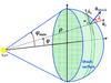 |
Fig. 7 Diagram representing the shock in spherical coordinates, assuming a symmetry of rotation around the Sun-apex direction. |
 |
Fig. 8 a) Synthetic probability distributions
|
3. A synthetic model of the 2D shock structure
3.1. A shock model with a spherical geometry
We found in Sect. 2 that the shock properties are
nearly independent of the angle i. This is compatible with a shock shape having a
symmetry of rotation around the axis going from the Sun to the shock apex. Then, we
describe the shock shape with the spherical coordinates (ρ,Φ,ϕ)
centered on the Sun (S), where Φ is the angle defining the position around the Sun-apex line. Because
of the supposed symmetry of rotation, the model is independent of Φ; hence only ρ and ϕ are shown in Fig. 7. A point M on the shock is located at 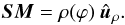 (3)The normal to the shock
is
(3)The normal to the shock
is 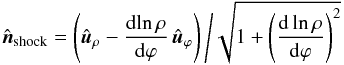 (4)with
the unit vectors
(4)with
the unit vectors  and
and
 defined in Fig. 7. Then, the location angle λ is related to
ρ(ϕ) as
defined in Fig. 7. Then, the location angle λ is related to
ρ(ϕ) as 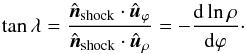 (5)We also suppose
that ρ(ϕ) is a decreasing function of
ϕ, so that
the shock is concave toward the Sun, as expected, if the ICME is not traveling in a very
structured (fast/slow/fast) solar wind (so we do not consider cases such as those
simulated by Manchester et al. 2004 where the front
is convex around the apex). Thus, λ is a monotonous increasing function of
ϕ. It
implies that spacecraft crossings in the range ϕ ± dϕ correspond to the unique
range λ ±
dλ. The conservation of the number of cases implies
(5)We also suppose
that ρ(ϕ) is a decreasing function of
ϕ, so that
the shock is concave toward the Sun, as expected, if the ICME is not traveling in a very
structured (fast/slow/fast) solar wind (so we do not consider cases such as those
simulated by Manchester et al. 2004 where the front
is convex around the apex). Thus, λ is a monotonous increasing function of
ϕ. It
implies that spacecraft crossings in the range ϕ ± dϕ correspond to the unique
range λ ±
dλ. The conservation of the number of cases implies
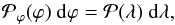 (6)where
 is the
probability of spacecraft crossing in the interval ϕ ± dϕ.
is the
probability of spacecraft crossing in the interval ϕ ± dϕ.
Coronal mass ejections are launched from the Sun from a broad range of latitudes and
longitudes. Moreover, the Sun is rotating, so that a spacecraft, which is at a given
distance D
from the Sun and is observing during years, is expected to cross ICMEs with a nearly
uniform distribution in both angular directions. Said differently, the probability of
detection of the shock in the range ϕ ± dϕ is proportional to the
corresponding fraction of the cross section of the sphere of radius D, so
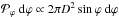 . Considering
shocks with a mean angular extension ϕmax, the normalization to 1 of the
total probability
. Considering
shocks with a mean angular extension ϕmax, the normalization to 1 of the
total probability  (integrated from ϕ =
0 to ϕmax) leads to
(integrated from ϕ =
0 to ϕmax) leads to 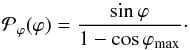 (7)Reporting this result in
Eq. (6) implies
(7)Reporting this result in
Eq. (6) implies 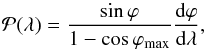 (8)which defines
 when the shock shape is known. The derivation of Eq. (5) with respect to λ defines dϕ/
dλ, and for a given shock shape, ρ(ϕ), the
probability
is computed as
when the shock shape is known. The derivation of Eq. (5) with respect to λ defines dϕ/
dλ, and for a given shock shape, ρ(ϕ), the
probability
is computed as 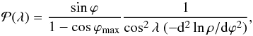 (9)where all terms can be
expressed as a function of λ. This is because ϕ can be expressed as a
function of λ
using Eq. (5) when ρ(ϕ) is
specified, as the example of Sect. 3.2.
(9)where all terms can be
expressed as a function of λ. This is because ϕ can be expressed as a
function of λ
using Eq. (5) when ρ(ϕ) is
specified, as the example of Sect. 3.2.
 |
Fig. 9 Synthetic probability distribution functions for the cosine model (see Sect. 3.2) showing three cases with the product nf = 0.3,1, and 1.5. All the distributions functions are varied as a function of ϕmax (pink to blue curves), showing the little influence of this free parameter on the distribution function. |
3.2. Derivation of the probability distribution of λ
In the following, we compute the distribution of the shock normal when a simple 2D shape
of the shock shell structure is given. We select the simplest shell structure in terms of
the number of free parameters and the complexity of the expression among several cases
explored. Still, this shape provides a probability ,
which has the main characteristics of the observed one,
,
for a range of parameter values. This modeled shape is expressed by means of a cosine
function as follows: 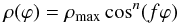 (10)with
f =
90°/ϕmax, so
that ρ(ϕmax) = 0. Then, the
shape is confined between the values
[−ϕmax,ϕmax]. This is a simple model since it only depends on the two parameters
f and
n.
(10)with
f =
90°/ϕmax, so
that ρ(ϕmax) = 0. Then, the
shape is confined between the values
[−ϕmax,ϕmax]. This is a simple model since it only depends on the two parameters
f and
n.
Developing lnρ, we obtain lnρ = lnρmax +
n lncos(fϕ). Computing
dlnρ/
dϕ relates ϕ to λ with Eq. (5) as 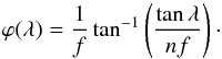 (11)A second
derivation of dlnρ/dϕ provides
(11)A second
derivation of dlnρ/dϕ provides
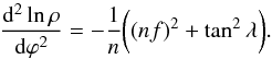 (12)With the
inclusion of this expression in Eq. (9),
the expression for
is rewritten as
(12)With the
inclusion of this expression in Eq. (9),
the expression for
is rewritten as 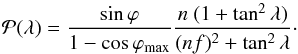 (13)With
ϕ expressed
using Eq. (11),
is explicitly a function of tanλ and then of λ. In the following, we
study the expected probability distribution functions from this cosine model by varying
two parameters: the product of nf and the free parameter ϕmax rather than
the original parameters, n and f, since the results are easier to describe with
these parameters.
(13)With
ϕ expressed
using Eq. (11),
is explicitly a function of tanλ and then of λ. In the following, we
study the expected probability distribution functions from this cosine model by varying
two parameters: the product of nf and the free parameter ϕmax rather than
the original parameters, n and f, since the results are easier to describe with
these parameters.
3.3. Synthetic probability distributions of λ
In Fig. 8, we show different synthetic probability
functions (left) for different nf values and the corresponding shock front shape
(right). The shape of the distribution function greatly changes, depending on the values
of nf. For
example, a slight variation from nf = 0.2 to 0.3 (pink to green curves) leads to a
decrease in the peak value of .
Moreover, the cases with nf ≥
0.6 show a probability distribution function that is too different from
,
as seen in Fig. 4, to be considered a possible
solution.
The right panels of Fig. 8 show half of the shock front shape that is deduced from the cosine model with the same ϕmax value. The front shock becomes flatter as nf decreases. In contrast, increasing nf to values >1 leads to shock front shapes that are more elongated in the radial direction with an ellipsoidal shape (not shown). Their corresponding distribution function is a monotonous increasing function of λ (Fig. 9c), which causes them to be incompatible with the observed distribution (Fig. 4).
The upper and lower panels in Fig. 8 are shown for
two different values of the free parameter ϕmax. Although changing this maximum
elongation of the shock leads to different shapes (right panels), the apex region is
similar from one case to another. This explains why the distribution functions are very
similar for the same nf values and with different values of
ϕmax. This result is better shown in Fig.
9, where the three panels show the synthetic
distribution function
for three sets with three different values of nf = 0.3,1,1.5.
Each set shows different
obtained by varying ϕmax from 15° to 90°. Varying this free parameter
does not significantly change the distribution functions. Then, the probability
distribution function is mostly governed by the product of nf. We find that the shapes
for the probability distribution function ,
which are consistent with ,
range between nf =
0.17 and nf
= 0.45.
In summary, we have derived a synthetic probability distribution function
with the present method from a simple cosine model, Eq. (10), that expresses the shape of the shock front in spherical
coordinates (assuming a rotation symmetry). It explicitly shows the tied link between the
shock shape and the probability .
We have found that this shape can explain the observed probability distribution functions
for a narrow range of nf, while the maximum elongation of the shock front,
ϕmax, has only a very weak influence on
the distribution functions. This analysis can be repeated with more complex models of the
shock shape, and one can search for the best fit to
.
This allows the deduction of the best shock shape from
within the range of models considered. Rather, we deduce the front shock shape by directly
integrating the observed probability distribution functions in the following part.
4. Deduction of the shock shape from the data
In the previous section, we have derived the probability distribution
for a shape of the shock that is described by a simple analytical function. Varying the free
parameters of the shock shape allows us to investigate which kind of
functions are to be expected. Still, the simple analytical function only allows the
reproduction of the main features of the observed
and differences with the model are present. Here we solve the reverse problem; that is, we
compute the shock shape from the observed .
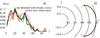 |
Fig. 10 a) Probability distributions |
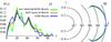 |
Fig. 11 a) Probability distributions |

4.1. Method
Similarly to Sect. 3, we suppose that the shock
shape has a rotation symmetry around the axis going from the Sun to the shock apex, and we
describe the shock shape with the spherical coordinates (ρ,ϕ) centered on the Sun
(S), as defined in Fig. 7. We also suppose that
ρ(ϕ) is a decreasing function of
ϕ, so that
the shock is concave toward the Sun. The probability of λ is derived from the
observations, so  .
The conservation of the number of cases, Eq. (6), relates
to
.
The conservation of the number of cases, Eq. (6), relates
to  ,
which is estimated by Eq. (7). Thus, Eq.
(6) writes
,
which is estimated by Eq. (7). Thus, Eq.
(6) writes  (14)After an
integration on ϕ, we take the arccos of this equation
(14)After an
integration on ϕ, we take the arccos of this equation 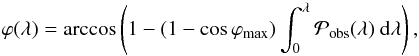 (15)which gives a relation
between ϕ and
λ through
the observed probability .
(15)which gives a relation
between ϕ and
λ through
the observed probability .
Next, we relate ρ to λ by combining Eqs. (5) and (14) to express
dlnρ/
dϕ. After integration, we obtain 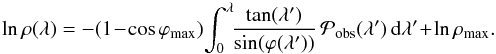 (16)The new parameter,
ρmax =
ρ(0), is only a constant factor for the deduced
shock shape. Setting the apex to 1 AU with ρ expressed in AU leads to lnρmax = 0 and
simplifies Eq. (16). Still,
sin(ϕ) is
present in the integral and should be expressed as a function of λ′ to continue
the integration. This is achieved with Eq. (15) written in function of λ′.
(16)The new parameter,
ρmax =
ρ(0), is only a constant factor for the deduced
shock shape. Setting the apex to 1 AU with ρ expressed in AU leads to lnρmax = 0 and
simplifies Eq. (16). Still,
sin(ϕ) is
present in the integral and should be expressed as a function of λ′ to continue
the integration. This is achieved with Eq. (15) written in function of λ′.
All in all, Eqs. (15) and (16) express the shape of the mean shock front
as parametric functions of λ in the spherical coordinates (ρ(λ),
ϕ(λ)). Apart from the scaling factor
ρmax that we set to 1 AU, there is one
intrinsic free parameter, ϕmax, which cannot be determined from
the in situ observations. Otherwise, the deduced shock shape depends only on two
integrations of functions that depend on the observed probability distribution
,
so the deduced shape is expected to weakly depend on statistical noise of
.
Moreover, we integrate the equations from the shock apex, λ = 0, to larger
λ values.
The region that is observed the best, which has more observed cases around the apex, is
not affected by the errors of
that are present at larger locations on the shock side. As a consequence of the data
properties and this integration procedure, the uncertainty in the deduced shock shape is
expected to grow approximately from its apex to its side.
4.2. Mean shock shape of ICMEs
The distributions
found in Fig. 4 are used in Eqs. (15) and (16) to deduce the most general shock shape. These two equations have
the same general characteristics as the ones derived for the MC axis (Eqs. (17) and (20)
of Janvier et al. 2013). Their differences are due
to the (2D) surface of the shocks compared to the (1D) curve of the MC axis. Their similar
characteristics, in particular the integrals on ,
also imply that the shock shape is very weakly affected by the type of interpolation used,
its order, and the number of bins present in the histogram of
(as in Fig. 10a of Janvier et al. 2013).
We further show here that the results are also weakly affected by the statistical
fluctuations of the bin count. For that, we select
derived from the shock associated to ICMEs, which has 91 shocks, or about half cases than
the total number (with and without associated ICMEs). We add statistical noise to the bins
of the observed
with an amplitude  where N is
the number of cases in the bin (with the constraint that the probability should be
positive). Because the number of cases in each bin is small (at most 11 cases), the
different realizations with added noise have large fluctuations, as shown with four
typical examples in Fig. 10a. Still, the deduced
shock shape is almost not affected (Fig. 10b). This
further shows that the results derived from Eqs. (15) and (16) are robust even if
is derived with a relative limited number of cases.
where N is
the number of cases in the bin (with the constraint that the probability should be
positive). Because the number of cases in each bin is small (at most 11 cases), the
different realizations with added noise have large fluctuations, as shown with four
typical examples in Fig. 10a. Still, the deduced
shock shape is almost not affected (Fig. 10b). This
further shows that the results derived from Eqs. (15) and (16) are robust even if
is derived with a relative limited number of cases.
Finally, we compare the shock shape deduced from three sets: first, shocks located in
front of ICME sheaths; second, shocks without any associated ICME (and away by more than 6
h from any ICMEs, and not inside an ICME or sheath); and third, the sum of both sets. The
lower probability for low λ values for the shocks without an associated ICME
(green curve) implies a slightly more bent shock shape (Fig. 11). However, this effect is negligible compared to the expected
variation from event to event (e.g., see Sect. 4.3).
Again, the derived shock shape is only affected by the global shape of
.
We also notice that we set ϕmax = 35° in Figs. 10 and 11, as
deduced in the next section from imager data for an observed ICME, but all the above
results are unchanged with other ϕmax values (which only rescales the
results in the ϕ direction).
4.3. Comparison with an ICME imaged by STEREO-B
We compare the mean shock shape below, which is deduced above from in situ data, with a well-observed ICME by both STEREO spacecraft on 1−6 June 2008. The evolution of the ICME was imaged from the Sun by the COR 1, 2 and HI 1, 2 instruments of STEREO-A, while STEREO-B crossed the flux-rope, providing in situ data (Möstl et al. 2009).
While this event was a slow CME (taking about 5 days to travel from the Sun to 1 AU), it is still preceded by a shock as detected in situ by STEREO-B. More precisely, the flux rope was traveling at a velocity ≈400 km s-1 and overtaking a slower solar wind at a velocity ≈330 km s-1; then a shock formed in front of the sheath (see Fig. 1 of Möstl et al. 2009). Indeed, the presence of a shock just in front of the sheath is typical of ICMEs that move significantly faster than the solar wind in front (Richardson & Cane 2010; Rouillard 2011, and references therein).
The dense plasma observed in situ in the sheath is at the origin of the bright features seen in imagers via Thomson scattering of the solar white light. Indeed, for this June 2008 event, Möstl et al. (2009) related both the front and rear (after the flux rope) sheaths, as observed in situ by STEREO-B, to the extrapolation in time of bright features present in the images of HI on STEREO-A. From this association, which was also shown in other events (Rouillard 2011, and references therein), we use the sharp intensity gradient in front of the leading sheath as a trace of the shock in the HI images.
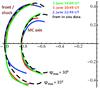 |
Fig. 12 Comparison of the shock/front and MC-axis shapes deduced from in situ observations (in dashed black lines) with the corresponding shapes of a flux-rope that is imaged by STEREO-A HI 1 (shown at three times with color lines, Möstl et al. 2009). The shock shape (dashed black line) is deduced from Eqs. (15) and (16) for fICME = − 1 to 2, while the front shapes are set at the largest gradient intensity in HI 1 images. The axis shapes are from Janvier et al. (2013). |
The HI images provide the elongation of the sheath front versus the latitude, which is a 2D projection of an unknown 3D plasma configuration. From this, the hypothesis should be made to estimate the 3D shape. We suppose that the observed brightening is part of an approximately spherical shell centered on the Sun; the observed 2D shape does not depend on the ICME direction. We convert the HI 1 observations to spatial positions by assuming a conic projection from STEREO-A on the plane of sky. Other approaches were considered, but this one was selected here because it implies the most believable results (see Sect. 5.2 of Janvier et al. 2013, where other hypothesis are tested).
The results at three times are compared with the shape deduced from in situ observations in Fig. 12. The apex of the front/shock is normalized to one to better compare the different shapes. This implies the rescaling of each shape by a constant factor. The apex of the MC axis is normalized to the mean value found in the STEREO-A observations and rescaled to the apex of the shock. The MC axis results are from Figs. 11 and 12a of Janvier et al. (2013), where the good correspondence between the mean axis shape deduced from in situ data with imager results was already noted with ϕmax ≈ 30°. A similar good correspondence is found for the shock shape with a slightly larger ϕmax (≈35°), as expected, since the shock is extending further away on the sides of the flux rope in MHD simulations. The imager results show some limited asymmetry, which is not present in the shape deduced by in situ data by construction (Sect. 4.1). The difference imager/in situ is typically increasing away from the apex (see Fig. 12). Moreover, there is a small temporal evolution with the two front shapes and MC-axis shapes found at a later time being closer to the shapes derived from in situ data.
All in all, it is remarkable that data from a different nature (in situ versus imagers, a sample containing a large number of ICMEs versus one case) provide so similar results (Fig. 12). Moreover, this is true for different types of in situ data (MC versus shock) with different data analysis to derive the MC axis and the shock normal. These results provide a coherent view of the typical shape of ICMEs, which is also comparable to the results of several MHD simulations. Finally, we leave more comparisons between different approaches to a future investigation.
5. Summary and conclusions
The present paper aims at deducing the most probable shape of the shock surface associated with ICMEs at 1 AU, which evolves during its propagation in the interplanetary medium. To do so, we propose a statistical approach using the list of Wang et al. (2010) for the shocks and the list of Richardson & Cane (2010) for the ICMEs. Neglecting the shock-like events observed by ACE, we were able to associate 117 in situ detected shocks to ICMEs and the remaining 99 shocks with no detected ICMEs behind. Interestingly, looking at the distribution of the different shock parameters, we found no evidence that shocks with no associated in situ-detected ICMEs are of a different nature from ICME-associated shocks. On the contrary, the strong similarities in the parameter distributions indicate that non-detected ICME shocks could be shocks that are crossed away from the ICME core or associated with a strongly eroded ICME (where the magnetic field has mostly reconnected with the surrounding interplanetary magnetic field).
We also introduced new angles to determine the normal vector to the shock: the inclination
angle i and the
location angle λ. Although both are related to the more common
longitudinal and latitudinal angles, these new angles allow us to directly define the
position of the shock crossing by the spacecraft with respect to the shock apex.
Interestingly, although the inclination angle has a uniform distribution, the location angle
distribution has a gamma-like distribution. The location angle distribution is used in the
following to extract information regarding the general shape of the shock shell. As a
further step to ensure the validity of the present study, we present different correlation
analyzes to study the possible correlations between λ and the other shock and
ICME parameters. Simple correlation analyzes, which give the Spearman and Pearson
correlation numbers, show that λ does not depend on any shock or ICME parameter. Next,
we investigated the possible changes of the probability distribution
.
For that, we studied the changes in the mean, median, and standard deviation values by
making subcategories of shocks, depending on the values of the shock or ICME parameters.
Since we found no significant tendency (apart from geometrical effects), this justified the
possibility to investigate all the shocks as a whole statistical sample, where we verified
the validity of our statistical approach.
We proposed two methods to deduce the general shape of shocks. Since these methods are based on the statistical analysis of a large sample of shocks, they only keep common features among the analyzed shocks and not the specific deformations of individual cases. In particular, there is no evidence of a systematic deformation of the mean shock shape in some privileged direction (e.g., east-west or north-south asymmetry). The shock observations are compatible with a mean shock shape having a rotational symmetry around the axis Sun-apex.
The first method describes a synthetic shape, which assumes a rotational symmetry around the axis of the shock shell. This synthetic shell is described in spherical coordinates and allows the expression of a synthetic probability for the location angle λ, given an expression for the shock shape. This shock shape in the present paper is given in terms of a cosine function and two parameters (n and f). We find that the product nf alone can define the shock shape. We show that we are able to find synthetic distributions that are very close to that obtained from the in situ observations by varying the product nf. Note that this is a generic method: we have chosen a cosine function among other possibilities, but this approach, which is simple in terms of equation complexity and number of parameters, allows the derivation of the general shape of the shock shell by exploring the parameter space of the model.
We also present another method as a second step where we directly integrate the observed
distribution of the location angle .
The spherical coordinates of the shock surface are expressed with the integrated probability
distribution without any given hypothesis (except the rotation symmetry) on the shock
structure. Interestingly, similar shapes to those found in the first step are deduced from
this second method, which prove the robustness and the consistency of the two approaches.
Finally, a last step consisting in the analysis of heliospheric images of a propagating MC with a shock front is given. In this step, the propagating structure shape is reported at different times during its evolution, and the shapes are directly compared with that found in the previous method. This method, which is also employed in Janvier et al. (2013) for the flux rope axis shape, has two consequences: on the one hand, it verifies the consistency of the previous methods where the shock shell was analyzed from in situ data, and on the other hand, it gives a constraint on one free parameter, the maximum elongation ϕmax, that cannot be constrained from the two previous methods. Following those different approaches, we were able to find the most probable general shape of the shock shell structure.
The presence of shocks and the associated sheath (i.e., post-shock material) at 1 AU can produce significant changes in the level of the magnetosphere-solar wind coupling (e.g., Wang et al. 2009,and references therein). The typical shock shape found in the present study can have several applications as follows.
A first application is to implement this structure in a space-weather forecast to predict the arrival time of a CME shock to a spacecraft or a planet. This problem was solved with an ideal spherical front by Möstl & Davies (2013). Replacing the spherical front by the mean shock shape found above can improve the prediction of the arrival time, especially on the flank parts where the deviation to a spherical model is the most important and the delay is the largest (up to two days in extreme cases).
Another application of the mean shock front is to determine a better crossing location of a shock, since the locally measured λ angle can be quantitatively converted to a position along the shock surface. This can be used to study the shock properties versus the apex distance if the shock is crossed by several spacecraft.
In addition, shocks can produce strong decreases of cosmic rays (e.g., the so-called Forbush decreases). Some Forbush events can present two-step developments, one of them non-local and produced by the shock. The other one is local and produced only during the passage of the ICME through the observer. The non-local step can last several days and is produced by a diffusive barrier created by the shock, even when the latter is far away from Earth. Knowing the general shape of the shock surface is crucial in determining the flux of cosmic rays reaching the terrestrial environment. This can be done, for instance, from the determination of the solid angle that the shock surface covers when seen from Earth. Results on the most probable shapes of the shock, as the ones shown in the present paper, will be important to improve quantitative models of cosmic rays modulation in the heliosphere, which at the moment are still controversial (Jordan et al. 2011). This has also space-weather applications because the input of high energy particles to the terrestrial environment can affect the dynamics of the magnetosphere-ionosphere system.
More insights on the evolution of the shocks and their propagation from solar sources, as given by the in situ instruments onboard Solar Orbiter, which will travel at closer distances to the Sun than the present heliospheric probes, will be of great interest in completing the present model of shock shapes.
Acknowledgments
M.J.’s work was partially funded by a research grant via the AXA Research Fund. S.D. acknowledges partial support from the Argentinian grant UBACyT 20020120100220. This work was partially supported by a one-month invitation of P.D. to the Instituto de Astronomía y Física del Espacio, and by a one-month invitation of S.D. to the Paris Observatory. S.D. is member of the Carrera del Investigador Científico, CONICET.
References
- Balogh, A., & Jokipii, J. R. 2009, Space Sci. Rev., 143, 85 [NASA ADS] [CrossRef] [Google Scholar]
- Balogh, A., Bothmer, V., Crooker, N. U., et al. 1999, Space Sci. Rev., 89, 141 [NASA ADS] [CrossRef] [Google Scholar]
- Barnden, L. R. 1973a, Proc. International Cosmic Ray Conf., 2, 1271 [NASA ADS] [Google Scholar]
- Barnden, L. R. 1973b, Proc. International Cosmic Ray Conf., 2, 1277 [Google Scholar]
- Berdichevsky, D. B., Szabo, A., Lepping, R. P., Viñas, A. F., & Mariani, F. 2000, J. Geophys. Res., 105, 27289 [NASA ADS] [CrossRef] [Google Scholar]
- Berdichevsky, D. B., Reames, D. V., Wu, C.-C., et al. 2009, Adv. Spa. Res., 43, 113 [NASA ADS] [CrossRef] [Google Scholar]
- Boursier, Y., Lamy, P., Llebaria, A., Goudail, F., & Robelus, S. 2009, Sol. Phys., 257, 125 [Google Scholar]
- Burlaga, L., Sittler, E., Mariani, F., & Schwenn, R. 1981, J. Geophys. Res., 86, 6673 [Google Scholar]
- Cane, H. V. 2000, Space Sci. Rev., 93, 55 [NASA ADS] [CrossRef] [Google Scholar]
- Cane, H. V., Richardson, I. G., von Rosenvinge, T. T., & Wibberenz, G. 1994, J. Geophys. Res., 99, 21429 [NASA ADS] [CrossRef] [Google Scholar]
- Cargill, P. J., & Schmidt, J. M. 2002, Ann. Geophys., 20, 879 [NASA ADS] [CrossRef] [Google Scholar]
- Dasso, S., Mandrini, C. H., Démoulin, P., Luoni, M. L., & Gulisano, A. M. 2005, Adv. Spa. Res., 35, 711 [CrossRef] [Google Scholar]
- Dasso, S., Mandrini, C. H., Démoulin, P., & Luoni, M. L. 2006, A&A, 455, 349 [NASA ADS] [CrossRef] [EDP Sciences] [Google Scholar]
- Dasso, S., Asorey, H., & Pierre Auger Collaboration 2012, Adv. Spa. Res., 49, 1563 [Google Scholar]
- de Lucas, A., Schwenn, R., dal Lago, A., Marsch, E., & Clúa de Gonzalez, A. L. 2011, J. Atmos. Sol. Terr. Phys., 73, 1281 [NASA ADS] [CrossRef] [Google Scholar]
- Farrugia, C. J., Berdichevsky, D. B., Möstl, C., et al. 2011, J. Atmos. Sol. Terr. Phys., 73, 1254 [NASA ADS] [CrossRef] [Google Scholar]
- Gosling, J. T., & Pizzo, V. J. 1999, Space Sci. Rev., 89, 21 [Google Scholar]
- Gosling, J. T., Bame, S. J., McComas, D. J., et al. 1995, Space Sci. Rev., 72, 133 [NASA ADS] [CrossRef] [Google Scholar]
- Gulisano, A. M., Démoulin, P., Dasso, S., & Rodriguez, L. 2012, A&A, 543, A107 [NASA ADS] [CrossRef] [EDP Sciences] [Google Scholar]
- Janvier, M., Démoulin, P., & Dasso, S. 2013, A&A, 556, A50 [NASA ADS] [CrossRef] [EDP Sciences] [Google Scholar]
- Jian, L., Russell, C. T., Luhmann, J. G., & Skoug, R. M. 2006, Sol. Phys., 239, 337 [NASA ADS] [CrossRef] [Google Scholar]
- Jian, L. K., Russell, C. T., Luhmann, J. G., Galvin, A. B., & MacNeice, P. J. 2009, Sol. Phys., 259, 345 [NASA ADS] [CrossRef] [Google Scholar]
- Jordan, A. P., Spence, H. E., Blake, J. B., & Shaul, D. N. A. 2011, J. Geophys. Res., 116, A11103 [NASA ADS] [CrossRef] [Google Scholar]
- Kilpua, E. K. J., Jian, L. K., Li, Y., Luhmann, J. G., & Russell, C. T. 2011, J. Atmos. Sol. Terr. Phys., 73, 1228 [Google Scholar]
- Lai, H. R., Russell, C. T., Jian, L. K., et al. 2012, Sol. Phys., 278, 421 [NASA ADS] [CrossRef] [Google Scholar]
- Lavraud, B., & Rouillard, A. 2014, in IAU Symp., 300, 273 [NASA ADS] [Google Scholar]
- Lee, C. O., Arge, C. N., Odstrčil, D., et al. 2013, Sol. Phys., 285, 349 [Google Scholar]
- Lin, C. C., Chao, J. K., Lee, L. C., Lyu, L. H., & Wu, D. J. 2006, J. Geophys. Res., 111, A09104 [NASA ADS] [Google Scholar]
- Lindsay, G. M., Russell, C. T., Luhmann, J. G., & Gazis, P. 1994, J. Geophys. Res., 99, 11 [NASA ADS] [CrossRef] [Google Scholar]
- Lugaz, N., & Roussev, I. 2011, J. Atmos. Sol. Terr. Phys., 73, 1187 [NASA ADS] [CrossRef] [Google Scholar]
- Manchester, W. B. I., Gombosi, T. I., Roussev, I., et al. 2004, J. Geophys. Res., 109, A02107 [Google Scholar]
- Manchester, IV, W. B., Vourlidas, A., Tóth, G., et al. 2008, ApJ, 684, 1448 [NASA ADS] [CrossRef] [Google Scholar]
- Masson, S., Démoulin, P., Dasso, S., & Klein, K.-L. 2012, A&A, 538, A32 [NASA ADS] [CrossRef] [EDP Sciences] [Google Scholar]
- Möstl, C., & Davies, J. A. 2013, Sol. Phys., 285, 411 [NASA ADS] [CrossRef] [Google Scholar]
- Möstl, C., Farrugia, C. J., Temmer, M., et al. 2009, ApJ, 705, L180 [NASA ADS] [CrossRef] [Google Scholar]
- Möstl, C., Farrugia, C. J., Kilpua, E. K. J., et al. 2012, ApJ, 758, 10 [NASA ADS] [CrossRef] [Google Scholar]
- Neugebauer, M. 2013, Space Sci. Rev., 176, 125 [NASA ADS] [CrossRef] [Google Scholar]
- Oh, S. Y., Yi, Y., & Kim, Y. H. 2007, Sol. Phys., 245, 391 [NASA ADS] [CrossRef] [Google Scholar]
- Richardson, I. G., & Cane, H. V. 2010, Sol. Phys., 264, 189 [NASA ADS] [CrossRef] [Google Scholar]
- Robbrecht, E., Patsourakos, S., & Vourlidas, A. 2009, ApJ, 701, 283 [Google Scholar]
- Rouillard, A. P. 2011, J. Atmos. Sol. Terr. Phys., 73, 1201 [Google Scholar]
- Ruffenach, A., Lavraud, B., Owens, M. J., et al. 2012, J. Geophys. Res., 117, A09101 [NASA ADS] [CrossRef] [Google Scholar]
- Sheeley, Jr., N. R., Howard, R. A., Michels, D. J., et al. 1985, J. Geophys. Res., 90, 163 [NASA ADS] [CrossRef] [Google Scholar]
- Simpson, J. A. 1954, Phys. Rev., 94, 426 [NASA ADS] [CrossRef] [Google Scholar]
- Siscoe, G., & Odstrcil, D. 2008, J. Geophys. Res., 113, A00B07 [Google Scholar]
- Smith, E. J. 2008, The global heliospheric magnetic field, eds. A. Balogh, L. J. Lanzerotti, & S. T. Suess (Chichester: Springer, Praxis Publishing), 79 [Google Scholar]
- Taubenschuss, U., Erkaev, N. V., Biernat, H. K., et al. 2010, Ann. Geophys., 28, 1075 [NASA ADS] [CrossRef] [Google Scholar]
- Vainio, R. 2009, in IAU Symp. 257, eds. N. Gopalswamy, & D. F. Webb, 413 [Google Scholar]
- Volkmer, P. M., & Neubauer, F. M. 1985, Ann. Geophys., 3, 1 [NASA ADS] [Google Scholar]
- Wang, C., Liu, J. B., Li, H., et al. 2009, J. Geophys. Res., 114, 5211 [CrossRef] [Google Scholar]
- Wang, C., Li, H., Richardson, J. D., & Kan, J. R. 2010, J. Geophys. Res., 115, 9215 [CrossRef] [Google Scholar]
- Xie, H., St. Cyr, O. C., Gopalswamy, N., Odstrcil, D., & Cremades, H. 2013, J. Geophys. Res., 118, 4711 [CrossRef] [Google Scholar]
- Xiong, M., Zheng, H., Wang, Y., & Wang, S. 2006, J. Geophys. Res., 111, 8105 [NASA ADS] [CrossRef] [Google Scholar]
All Figures
|
Fig. 1 Geometry of a shock propagating from the Sun and related-orientation parameters in
the heliocentric coordinates: a) the shock surface and the normal vector
|
| In the text | |
|
Fig. 2 a) Distribution of the inclination angle i (see Fig. 1b) for shocks detected by ACE and for 24 bins. b) i distribution for the same set of shocks with a selection on λ as: 30° ≤ λ ≤ 90°. |
| In the text | |
|
Fig. 3 Distributions of a) the ratio of the downstream density over the upstream density ρ2/ρ1, b) the upstream fast-mode Mach number Mf1, and c) the shock speed Vsn for fICME = − 1, which has no associated ICME in situ detected. Distributions of d) ρ2/ρ1, e) Mf1, and f) Vsn for all shocks related with an in situ detected ICME (fICME = 0,1or2). |
| In the text | |
|
Fig. 4 a) Distribution of the location angle λ (see Fig. 1) for fICME = −1, which has no associated ICME in situ detected. The distribution is given for a bin size Δλ = 4.5°. b) Distribution of λ with same bins for all shocks related with ICMEs (fICME = 0,1 or 2). |
| In the text | |
|
Fig. 5 Top: correlation between λ and ρ2/ρ1 for a) non-detected ICME shocks (fICME = − 1) and b) shocks associated with ICMEs (fICME = 0,1 and 2). The correlation is very weak for both cases. Middle: correlation between λ and the shock speed Vsn for c) non-detected ICME shocks and d) shocks associated with ICMEs. The correlation between the two parameters is very large, and the same tendency is found for different types of shocks. This tendency is compatible with Vsn∝ cosλ (green dashed lines). Bottom: e) correlation between λ and the ICME ΔV (difference between the front and the rear velocities), and f) correlation between λ and Dst for shocks with ICMEs. |
| In the text | |
|
Fig. 6 Median of |
| In the text | |
|
Fig. 7 Diagram representing the shock in spherical coordinates, assuming a symmetry of rotation around the Sun-apex direction. |
| In the text | |
|
Fig. 8 a) Synthetic probability distributions
|
| In the text | |
|
Fig. 9 Synthetic probability distribution functions for the cosine model (see Sect. 3.2) showing three cases with the product nf = 0.3,1, and 1.5. All the distributions functions are varied as a function of ϕmax (pink to blue curves), showing the little influence of this free parameter on the distribution function. |
| In the text | |
|
Fig. 10 a) Probability distributions |
| In the text | |
|
Fig. 11 a) Probability distributions |
| In the text | |
|
Fig. 12 Comparison of the shock/front and MC-axis shapes deduced from in situ observations (in dashed black lines) with the corresponding shapes of a flux-rope that is imaged by STEREO-A HI 1 (shown at three times with color lines, Möstl et al. 2009). The shock shape (dashed black line) is deduced from Eqs. (15) and (16) for fICME = − 1 to 2, while the front shapes are set at the largest gradient intensity in HI 1 images. The axis shapes are from Janvier et al. (2013). |
| In the text | |
Current usage metrics show cumulative count of Article Views (full-text article views including HTML views, PDF and ePub downloads, according to the available data) and Abstracts Views on Vision4Press platform.
Data correspond to usage on the plateform after 2015. The current usage metrics is available 48-96 hours after online publication and is updated daily on week days.
Initial download of the metrics may take a while.