| Issue |
A&A
Volume 565, May 2014
|
|
|---|---|---|
| Article Number | A87 | |
| Number of page(s) | 13 | |
| Section | Interstellar and circumstellar matter | |
| DOI | https://doi.org/10.1051/0004-6361/201323205 | |
| Published online | 16 May 2014 | |
Ionization structure of multiple-shell planetary nebulae
I. NGC 2438⋆
1 Institute for Astro and Particle Physics, Leopold Franzens Universität Innsbruck, Technikerstrasse 25, 6020 Innsbruck, Austria
e-mail: This email address is being protected from spambots. You need JavaScript enabled to view it.
2 Instituto de Astronomía, Universidad Católica del Norte, 0610 Avenida Angamos, Antofagasta, Chile
e-mail: This email address is being protected from spambots. You need JavaScript enabled to view it.
3 Jodrell Bank Centre for Astrophysics, School of Physics and Astronomy, University of Manchester, Manchester M13 9PL, UK
e-mail: This email address is being protected from spambots. You need JavaScript enabled to view it.
Received: 6 December 2013
Accepted: 26 March 2014
Abstract
Context. In recent times an increasing number of extended haloes and multiple shells around planetary nebulae have been discovered. These faint extensions to the main nebula trace the mass-loss history of the star, modified by the subsequent evolution of the nebula. Integrated models predict that some haloes may be recombining, and thus are not in ionization equilibrium. But parameters such as the ionization state and thus the contiguous excitation process are only poorly known. The haloes are very extended, but faint in surface brightness −103 times lower than the main nebula. The observational limits call for an extremely well studied main nebula, to model the processes in the shells and haloes of one object. NGC 2438 is a perfect candidate to explore the physical characteristics of the halo.
Aims. The aim is to derive a complete data set of the main nebula. This allows us to derive the physical conditions from photoionization models, such as temperature, density and ionization, and clumping. These models are used to derive whether the halo is in ionization equilibrium.
Methods. Long-slit spectroscopic data at various positions in the nebula were obtained at the ESO 3.6 m and the SAAO 1.9 m telescope. These data were supplemented by imaging data from the HST archive and from the ESO 3.6 m telescope and by archival VLA observations. The use of diagnostic diagrams draws limits for physical properties in the models. The photoionization code CLOUDY was used to model the nebular properties and to derive a more accurate distance and ionized mass.
Results. We derive an accurate extinction EB − V = 0.16, and distance of 1.9 ± 0.2 kpc. This locates the nebula behind the nearby open cluster M46 and rules out membership. The low-excitation species are found to be dominated by clumps. The emission line ratios show no evidence for shocks. The filling factor increases with radius in the nebula. The electron densities in the main nebula are ~250 cm-3, dropping to ~10−30 in the shell. We find the shell in ionization equilibrium: a significant amount of UV radiation infiltrates the inner nebula. Thus the shell still seems to be ionized. The spatially resolved CLOUDY model supports the hypothesis that photoionization is the dominant process in this nebula, far out into the shell. Previous models predicted that the shell would be recombining, but this is not confirmed by the data. We note that these models used a smaller distance, and therefore different input parameters, than derived by us.
Key words: planetary nebulae: general / planetary nebulae: individual: NGC 2438 / stars: AGB and post-AGB
Based on observations at ESO, SAAO and VLA, and HST archive.
© ESO, 2014
1. Introduction
Planetary nebulae (PNe) are the ionized ejecta from an asymptotic giant branch (AGB) star. They are a short-lived phenomenon compared with a typical stellar lifetime, and are visible while the now post-AGB star crosses the Hertzsprung-Russell diagram (HRD) toward high temperatures before entering the white-dwarf cooling track. Most of the luminous material originates from the stellar wind during the last thermal pulses on the AGB.
We investigate the physical conditions of a special type of PNe: Multiple-shell planetary nebulae (MSPNe), which are surrounded by faint outer shells and/or haloes. In recent times, an increasing number of haloes and multiple shells around PNe have been discovered. Although MSPNe are a familiar phenomenon, most of them are hardly studied and poorly understood. Previous research (e.g., Corradi et al. 2003; Zhang et al. 2012; or Ramos-Larios et al. 2012a,b) identified MSPNe as a common feature for nearly round nebulae. They appear during the evolution at about the knee in the HRD and in the early part of the cooling track. The observed MSPN structures are the intricate result of the interaction of hydrodynamic and radiative processes during both the AGB and the post-AGB phases. A detailed description of the mass-loss history and the connection between the stellar winds and the huge extended circumstellar envelopes can be found in for example Blöcker (1995) and Decin (2012). Owing to the faintness of the haloes, up to a factor of 103 lower than the main nebula in surface brightness, most of them were discovered much later than the nebula itself.
Corradi et al. (2000), Schönberner & Steffen (2002), and Perinotto et al. (2004) used 1D radiative transfer hydrodynamic (RTH) models to calculate the evolution of this type of nebulae. They modeled the full evolution of the PN starting at the AGB in a sophisticated way. These important models provide a very good representation of the surface brightness of MSPNe at an age of about 10 000 years. The RTH models result in outgoing shock fronts. At an age of about 10 000 years (assuming the Blöcker (1995) track of an 0.605 M⊙ central star), the resulting density profile peaks at  500 cm-3 (and thus
  560 cm-3). The central star of the PN (CSPN) has a luminosity of ≈250 L⊙ and a temperature of TCSPN ≈ 120 kK. In these models, the outer limit of the bright nebula is the limit of the hard UV radiation – a radiation-bounded optically thick PN. The shell material is nearly recombined (ne:nH = 1:10), with a temperature of 2000 K. Thus the [O i] λ6300 Å line is predicted to be about six times stronger than H β.
These types of models are enormously important for the general understanding of the evolution. The layered structure predicted by the models compares well with observations. In this paper, we investigate the ionization structure of an MSPN to provide observational constraints for the models.
We use the nomenclature introduced by Chu et al. (1987) and Balick et al. (1992), but fully defined by Corradi et al. (2003), based on the evolutionary RTH models:
-
the main nebula − in literature also sometimes called rim;
-
the first thin surrounding structure including its outer weak intensity-enhancement is called shell;
-
the faint outer structures are called halo1 and halo2.
The only observational study of the nebula over a wide optical wavelength range and through the whole main nebula was obtained by Guerrero & Manchado (1999), with a single exposure at the ESO 1.5 m telescope. They centered the list on the brightest star near the center (not the CSPN), and integrated over wide areas along the slit. Guerrero & Manchado (1999) reported no detection of the [O i] line. This might be due to the strength of the telluric airglow line at this position. Earlier studies of the innermost regions around the CSPN were made by Torres-Peimbert & Peimbert (1977), Kaler (1983), Kingsburgh & Barlow (1994), and Kaler et al. (1990). All of them were focusing on abundances and found a mild helium and nitrogen overabundance.
The spectral investigation of Corradi et al. (2000) covered the regions of [O iii] λ5007 Å and H α + [N ii] λ6548 Å + λ6584 Å with a high resolution of 70 000. They provided good results for the expansion of the nebula.
The CSPN was investigated in detail by Rauch et al. (1999), using non-local thermodynamic equilibrium (NLTE) stellar atmosphere models. The results are log (g [cgs] ) = 6.62 ± 0.22, TCSPN = 114 ± 10 kK, LCSPN = 570 L⊙, and MCSPN = 0.56 ± 0.01 M⊙. The helium overabundance of the CSPN is slightly higher than found in the studies of the inner nebula mentioned before. Rauch et al. (1999) reported that the nebula luminosity is an order of magnitude higher than the luminosity of the CSPN. We later show (see Sect. 4), that this discrepancy was not caused by the model, but by the photometry from the literature they used. The low CSPN mass would imply a slow post-AGB evolution.
Based on the line ratios of [O iii]:He ii:H i in the main nebula and the line ratio of [O iii]:H i in the shell, photoionization studies (Armsdorfer et al. 2002, 2003) stated that the shell consists of ionized material. The required amount of ionizing UV photons can be obtained by a clumpy structure of the main nebula, allowing UV photons to escape. Such structures are established for some well-studied PNe such as the Helix Nebula (O’Dell et al. 2005; Matsuura et al. 2009) or the Ring Nebula (Speck et al. 2003; O’Dell et al. 2003). In Dalnodar & Kimeswenger (2011), the positions of the spokes of enhanced intensity in the shell of NGC 2438 was shown to be correlated to holes in the main nebula. This supports the concept of a matter-bounded structure. Recent studies of the MSPN IC 418 (Ramos-Larios et al. 2012a) and NGC 6369 (Ramos-Larios et al. 2012b) revealed very similar results: “Radial filaments emanate outwards from most of the [N ii] knots”.
We compiled our own spectroscopy and multiwavelength imaging data sets. Combining more information and data gives us the opportunity to search for the origin of the reported discrepancies and to draw detailed constraints for multidimensional RTH studies of MSPNe. We analyzed long-slit spectra, narrow-band images, a VLA radio map, and HST archival data. We investigated the main nebula and the shell by means of a sophisticated spatially resolved CLOUDY model (Ferland et al. 1998, 2013).
2. Observations and data reduction
2.1. Spectroscopy
Two independent spectroscopic data sets of NGC 2438 were used. The first spectroscopic data set was taken at the European Southern Observatory (ESO) at La Silla in Chile. Observations during three nights in 1996 were obtained, using the 3.6 m telescope and the ESO Faint Object Spectrograph and Camera (EFOSC11) in long-slit mode. The slit was positioned across the CSPN. These observations are summarized in Table 1.
The second spectroscopic data set was taken 2002 at the South African Astronomical Observatory (SAAO) 1.9 m Radcliffe Telescope in Sutherland. The observations were obtained during four nights. Because of the short slit, several positions were taken – scanning the whole nebula. These observations are summarized in Table 1. The slit positions are indicated in Fig. 1.
All instrumental parameters of the two observations and all the technical details are summarized in Table 2.
Spectroscopic data set.
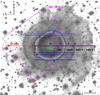 |
Fig. 1 Overview of the target observations. The background image is an H α EFOSC1 image. The spectrograph slits were all positioned in the E-W direction. The SAAO slit numbers correspond to those in Table 1. The CSPN and the region names as defined in Sect. 1 are shown and the field of view of the HST WFPC2 images is indicated as well. |
Technical details and instrumental parameters.
The spectra were reduced by standard MIDAS (Warmels 1991) routines. We corrected for variations of the slit width along the slit by adding the flatfield images. The variations were of about 2% in the EFOSC1 spectra and up to 17% in the SAAO spectra. The variations show no dependency on wavelength. As the outer haloes are not visible east of the nebula in the ESO data, the night sky could be taken directly from the spectra. For the SAAO data, the sky was taken from the slit positions outside the nebula and the shell. Additionally, the sky for the SAAO data could be taken from data from other, smaller nebulae, which were observed by Thomas Rauch during the same nights. These other PNe without halo were used to estimate straylight contamination of the surroundings. Both instruments show no contamination down to the noise level of the images. For the extraction of the nebular lines and proper suppression of local free-free continuum, the nearest empty region along the slit was used. Typically, the nearest region was directly redward and blueward of each line. In some cases only one side was used, to avoid blending with other lines. To improve the signal to noise ratio (S/N), the width of the region was three times larger than the FWHM of the lines. The contribution was found to be fairly small within the main nebula. Only at the very blue end the readout noise was detected a few times. Outside the main nebula, toward shell and halo, no variation higher than the sky level within the limits of the readout noise was detected.
Corrections for differential refraction were applied on both data sets, using the algorithm of Fluks & The (1992). These corrections were applied to the standard stars and to the CSPN spectra to obtain the absolute flux calibrations. Because the observations were made near zenith, the corrections for the nebula are very small and the effect of variation of the parallactic angle during the long nebula exposures are negligible. For the standard stars, we only have exposures of 1 and 5 min, during which the parallactic angle was constant. The differential refraction correction is at most 9% at the blue end of the spectra.
After applying all corrections from night to night, the flux differences of the standard stars were only a few percent. For overlapping observations between the SAAO and the ESO spectra, a variation below 5% of the bright lines (e.g., [O iii]) was found. For the fainter lines (e.g., Ar ii, H δ), a typical variation of less than 10% was found. Taking conservative estimates of systematic effects, we assume the overall absolute flux accuracy to be better than 12% in the main nebula, and better than 20% in the shell. Differential values (e.g., line ratios) are expected to be better than 5%.
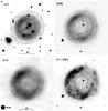 |
Fig. 2 Direct images of the main nebula. First row: He ii (λ4686 Å) and [O iii] (λ5007 Å); second row: VLA (20 cm) and H α (λ6563 Å) +[N ii] (λ6548 Å+λ6584 Å) (same orientation as shown in Fig. 1− N is up, E is left). The ellipses are derived from the images of the He ii line. While the He ii emission is clearly concentrated towards the inner edge of the main nebula, the [O iii] and VLA images have about the same appearance. |
2.2. Imaging
Direct images using narrow-band filter [O iii] λ5007 Å (ESO filter #686), He ii λ4686 Å (ESO filter #512) and H α + [N ii] λ6548 Å/λ6584 Å (ESO filter #691) were obtained at the ESO 3.6 m telescope. The absolute flux calibration was scaled from the long-slit spectra. The H α filter #691 contains significant contributions of both [N ii] lines. The filter response was used to derive a sensitivity of 95% of the λ6548 Å line and 75% of the λ6583 Å line (relative to peak transmission).
As a byproduct of an investigation of the nearby bipolar nebula OH 231.8+4.2 (Taylor & Morris 1993), VLA radio observations of NGC 2438 were obtained and made available to us by the authors.
The morphologies in the different images show variations (Fig. 2). In the [O iii] image and in the VLA image, the same nebula structures, elongation, and central cavity were found. The He ii image shows more concentration toward the inner region. Despite the Bowen fluorescence, the decoupling of the helium and oxygen image shows the limit of the optically thick region in the helium Lyman continuum, used in the modeling part (Sect. 6). The (H α+[N ii]) image is dominated by substructures and clumps. The rim of the main nebula is slightly elongated by about 0.9:1 (Fig. 2). The ellipticity is fairly low (0.84, 0.91 and 0.94 from inner to outer ellipse) and the position angles are constant.
Additionally, a data set of NGC 2438 in the HST archive was retrieved. The images, taken in September 2008, do not cover the whole nebula. The data set is summarized in Table 3. The inner region was covered by the high-resolution PC camera and has a very low S/N. The images are not deep enough to show structures of the shell or the haloes (Fig. 3). They were used to analyze shock signatures (see Sect. 5.3).
The post-flight measurements of the WFPC2 filters, the expansion velocity, and the systematic velocity measured by Meatheringham et al. (1988) and by Corradi et al. (2000), were used to calculate the effect of the line width on the filter transmission. We obtained a contamination by [N ii]λ6548, and [N ii]λ6584 in the F656N filter band of 39% and 2%, respectively. In contrast, the F658N filter has a sensitivity of just about 1.7% for H α. Both filters have the same peak transmission. Thus we were able to directly obtain a pure H α image, using the image of F658N and the known line ratio of [N ii]λ6548/[N ii]λ6584. This H α image shows exactly the same morphology as the [O iii] image and VLA image shown before. The [N ii] image and the [S ii] image indicate identical structures throughout all regions of the nebula. Additionally, the [O iii] and the H α images show some cometary knots and ray-like structures pointing outwards of the edges (Fig. 4). The shadow tails of the knots, pointing exactly away from the CSPN as result of the shielding of hard UV, are clearly visible only in [O iii]. The radiation to ionize the H i is provided by the diffuse nebula radiation, thus no shadows are formed in H α.
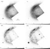 |
Fig. 3 HST images of the main nebula. First row: [O iii](λ5007 Å) and H α after subtracting [NII] contribution (see text); second row: [N ii] (λ6584 Å) and [S ii](λ6716 Å+λ6732 Å). The images are in the same orientation as shown in Fig. 1 and cover the field of view shown there. The similarities in the structures are obvious. |
3. Extinction and CSPN parameters
The foreground extinction towards the nebula was derived using the Balmer line series in the SAAO spectra. The intrinsic line intensities Rintr for the case B recombination calculated by CLOUDY and the interstellar extinction curve from Osterbrock & Ferland (2006) of the four isolated Balmer lines from λ4102 Å to λ6563 Å were used to derive the interstellar foreground extinction from the measured line ratios R by
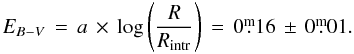 The intrinsic line ratios Rintr were determined iteratively, starting with Te = 10 kK, taken from the table in Osterbrock & Ferland (2006), and calculated with CLOUDY using the temperature derived from the N ii lines (see Sect. 6, Table 6). The final CLOUDY model gives additional information about the blended He ii lines. The flux contribution at these temperatures is only 1−3%. Thus the error introduced for line ratios by neglecting the contribution of the He ii lines is expected to be in the order of only 1%. As shown in Table 4, all line ratios lead to the same extinction. Thus the assumptions of case B recombination and standard extinction apply very well. The spread is remarkably small.
Observation log of the HST archival images (all taken with WFPC2).
Extinction measurement with the Balmer lines.
To search for intrinsic extinction in the nebula, the spatial distribution of the ratio R was investigated. We used H α from the SAAO data, and H β from the ESO data, as they are deeper in the outer shell (Fig. 5). The results show no correlation in the position and the line intensity. Even in the thin shell the same ratio was found.
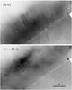 |
Fig. 4 Zoom of the N-E region of the main nebula from the HST images. The cometary knots are especially pronounced in the [O iii] images. The shadows point exactly away from the CSPN (direction indicated by two lines). |
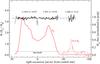 |
Fig. 5 The spatial distribution of the line ratio R = Hα/Hβ to search for intrinsic extinction. To cover homogeneous S/N ratios, a threshold of 3.5× below the S/N peak was chosen. Also the region around the CSPN was excluded. For the shell, the same procedure was applied, but 20× fainter. |
Guerrero & Manchado (1999) derived an extinction of 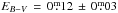 . They noted that their solution of the series does not fulfill the theoretically expected values for such plasmas after de-reddening. To obtain a reasonable S/N ratio, they integrated over large regions along the slit. The off-centered slit leads to non-radial terms in the integrated line intensities. Taking into account the offset of their slit, we find a fair agreement at the blue end.
A spectroscopic comparison of the hot white dwarf (WD) standard star EG 274 and the CSPN leads to an independent test of the calibration. The CSPN was completely covered by the ESO spectra and by three spectra (3, 4, and 9) in the SAAO data set. The combined information from three different nights and two different instruments reduces the calibration errors and excludes systematic effects in the data reduction. The de-reddened SAAO spectrum, overlayed with the WD spectrum of the standard star EG 274, shows the high accuracy of the extinction value and of the calibration over the whole wavelength range (Fig. 6). Thus we were able to use this to secure the photometry. The CSPN flux at λ5500 Å is 2.3 × 10⁻¹³erg cm-2s-1Å-1 with an rms of 5%. Using the zero point by Colina et al. (1996), we obtained values of  , and
, and  for the CSPN.
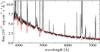 |
Fig. 6 CSPN (thin black line) without removing the nebula emission lines, and the standard star EG 274 overlayed (smooth red line − scaled and the extinction |

4. Distance determination
There are several distance estimates of NGC 2438 in the literature, leading to values between 0.8 and 4.3 kpc.
Rauch et al. (1999) used the spectroscopy of the central star to derive temperature and surface gravity. They used V = 18 0, from Acker et al. (1992), and a reddening in the range of
  . This leads to a large distance of 4.3 kpc and large errors. Using the CSPN parameters and the extinction derived in this work (see Sect. 3), we obtained a new spectroscopic distance of
  kpc with their model.
For the open cluster M 46 on the same line of sight, a distance of 1.51 kpc (Sharma et al. 2006) is given from optical CCD photometry with  . Using infrared 2MASS data leads to an extinction of
  and a distance of 1.7 ± 0.25 kpc (Majaess et al. 2007). The abundance of [Fe/H] = −0.03 (Paunzen et al. 2010) is very near to solar and the cluster is very rich. The fits of the evolutionary tracks and thus the distances and extinction values are reliable. Our extinction value places the PN behind the cluster. This result agrees with Kiss et al. (2008), who already rule out a cluster membership of the PN because of the large discrepancy in the radial velocity.
Radio observations yield distance estimators based on a number of distance scales with different assumptions and calibration. Using the high-resolution VLA radio map of Taylor & Morris (1993), we derived a radio flux of 74.9 ± 1.6 mJy at a frequency of 1.5 GHz (20 cm). This is slightly lower than the result of 80.3 ± 3.2 mJy, given in the NVSS (Condon et al. 1998). The difference arises because of the background source at 07h39m35 8s−14°28′04′′ was not resolved by the survey. Using survey data from NVSS, PMN, and F3R, the radio spectral energy distribution (SED) can be fit by a pure free-free radiation (Vollmer et al. 2010). Thus using I = I0ν-0.1 we derived a radio flux of S6 cm = 66 mJy. This corresponds well to the S6 cm = 67 mJy, given by Zijlstra et al. (1989) in their VLA survey. Using the calibration of van de Steene & Zijlstra (1995) of the radio continuum brightness temperature, we obtained a distance of 1.8 ± 0.3 kpc. The scale by Bensby & Lundström (2001) results in 2.1 ± 0.3 kpc. The errors mainly originate in the way we determined the radius. We used the 20% contour level of the H i and the [O iii] image, averaged over the ellipticity. The errors are estimates, varying inwards to the slightly smaller VLA image and outwards to the 5% level of the optical images. The statistical distance scale of Schneider & Buckley (1996) results in a lower distance of about 1.2 kpc. But such low distances tend to be excluded by the extinction derived for the nebula and for the open cluster M 46.
Considering the individual spectroscopic distance and the distance of M 46 as a foreground object, we adopt a distance of 1.9 ± 0.2 kpc for NGC 2438. The error estimate makes use of the fact that Majaess et al. (2007) and Paunzen et al. (2010) found no intrinsic extinction variations in M 46, and thus NGC 2438 has to be beyond the cluster. This is consistent with the nebula distance scale reported by van de Steene & Zijlstra (1995) and Bensby & Lundström (2001). Other statistical distance scales, giving results around 1 kpc, have to be excluded because of the values found for the open cluster M 46. The resulting dimensions of the nebula are summarized in Table 5.
Dimensions of the nebula, derived for a distance of 1.9 kpc.
5. Spectral analysis
5.1. General appearance
The combined nebular spectra at the slit position through the CSPN are shown in Fig. 7. The spectra obtained at the other positions were compared with the combined spectra at the center, as a function of distance from the CSPN. The variations between different lines are slight. Only the clumpy low-excitation species [N ii] and [S ii] vary by up to a factor of 2 in their line ratios. This compares well with the results of the imaging and the radio observations (see Fig. 2). The profiles show three groups:
-
The high-excitation species (level >30 eV or ionization >60 eV) are concentrated at the center.
-
The medium-excitation species (level >10 eV or ionization >20 eV) are smoothly distributed over the whole nebula.
-
The low-excitation species (levels <5 eV and single ionized or neutral) are dominated by clumps.
Only the triplet He iλ4472 Å line and the singlet He iλ6678 Å line do not follow because of the extreme long lifetime of the He i 3S (19.82 eV) state of the singlet fake a kind of ground state and do not behave according to the criteria given above.
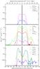 |
Fig. 7 Various lines of the nebula (logarithmic representation). The different spectral regions originate from different spectra (ESO and SAAO) and thus vary in S/N ratio at similar physical intensities. The panels show the excitation groups (criteria see text). The high-excitation species (upper panel) concentrate at the central region. The medium-excitation species (middle panel) smoothly follow the total brightness and the radial behavior of the VLA image throughout the nebula. The low-excitation species (lower panel) are dominated by clumpy structures. The O ii λ3729 is at the edge of the CCD and its flux calibration is very uncertain. It is added only for comparison of the profiles. |
Although He ii and [O iii] are coupled via the Bowen fluorescence, the spatial profiles of these two elements differ. But within one group, the profiles are identical.
These groups and the behavior of the low-excitation species are similar to those described by Ramos-Larios & Phillips (2012) for the PN NGC 2371. It also resembles the H α:[N ii] surface brightness profiles of NGC 6369 (Ramos-Larios et al. 2012b). The change of the excitation gives strong constraints for the optical thickness in the models (see Sect. 6).
5.2. Density distribution and electron temperature
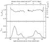 |
Fig. 8 Density derived from [S ii], in E-W direction through the CSPN. The line ratio (upper panel) and the electron density is nearly constant. The density profile does not follow the strong surface brightness variations (lower panel). |
The diagnostic density and temperature diagrams (described in Osterbrock & Ferland 2006 and Proxauf et al. 2014) provide the input and boundary conditions. Despite the strong variation in intensity, the density derived with [S ii] results in a flat distribution (Fig. 8), with values of 200 ≤ ne ≤ 300 cm-3. This corresponds well with the value of 300 cm-3 calculated by Meatheringham et al. (1988), who used the O iiλ3727Å/λ3729Å doublet and integrated the whole nebula. The two detections suffer from the fact that only low-excitation species were used.
Near the peak intensity of the main nebula, we were even able to detect Cl iii λ5517 Å/λ5537 Å. Throughout a large fraction of the whole nebula, we found Ar iv λ4711 Å/λ4740 Å. The two doublets reflect the density of the high-excitation plasma. However, as shown in Stanghellini & Kaler (1989) and in Copetti & Writzl (2002), these lines are only suited for slightly higher densities. An upper limit of the density of 300 to 400 cm-3 is stated.
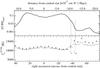 |
Fig. 9 Intensity (upper panel) of the [O iii] λ5007 Å, and the electron temperature using [O iii] (λ4958 Å+λ5007 Å)/λ4363 Å ratios along the slit (lower panel). The logarithmic scale is used to show the shell and the even farther extended halo. The flux scale is the same as in Fig. 7. The plus signs indicate the solution by exponential formula of Osterbrock & Ferland (2006). The bars give the solution using the new calibration of Proxauf et al. (2014). |
The [O iii] (λ4958 Å+λ5007 Å)/λ4363 Å ratios along the slit result in an electron temperature of 10 000 to 11 500 K in the main nebula. An increase in the shell is suggested (see Fig. 9). The transition to the shell is marked by dashed lines with 1/10 and 1/100 of the peak intensity. The result reaches up to 13 000 K according to the new calibration of Proxauf et al. (2014). Because of the weakness of the [O iii] λ4363 Å, which is about 100 times fainter than the [O iii] λ5007 Å emission, this may be an overestimation. There is no indication for a significant decline in temperature, as would be expected for a recombining halo. The presence of the λ4363 line (>5 eV) confirms a high temperature.
Only in the main nebula we were able to derive the [N ii] (λ6548 Å+λ6583 Å)/λ5755 Å line ratios. The results are very close to that of [O iii] (see Table 6). This implies that we see the same material of the nebula in two different excitation states. A third temperature diagnostic is given by Keenan et al. (1988), using Ar iii (λ7135 Å+λ7751 Å)/λ5192 Å. Unfortunately, our spectral resolution is insufficient to detect Ar iii λ5192 Å in the blend with the N i λ5198 Å+λ5200 Å lines.
Parameters of the target and of the best-fit model of the main nebula (14′′−38′′).
5.3. Searching for shock signatures
As the radiative transfer hydrodynamic (RTH) models predict shocks during certain stages of the evolution (Corradi et al. 2000; Schönberner & Steffen 2002; Perinotto et al. 2004), we searched carefully for shock signatures to exclude possible regions where the photoionization model does not work.
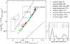 |
Fig. 10 Diagnostic diagram of the separation of shocked nebulae from photoionized PNe (after Magrini et al. 2003). The points follow the sequence of the ionization class toward the center. The dashed line gives a fit through the good data points (filled symbols). No dependency on increase or decrease of the intensity can be found (small panel). |
Originally shown by García Lario et al. (1991) and later investigated more in detail by Magrini et al. (2003), the ratios of log (H α/[N ii]) vs. log (H α/[S ii]) can be used to separate photoionized PN plasma from shocked gas, as seen for instance in supernova remnants (SNRs). Schmeja & Kimeswenger (2001) have shown that for photoionized gas of symbiotic Miras, the position in the diagram is an indicator of the level of excitation as well. The spectra of the main nebula of NGC 2438 clearly show the excitation tendency from inside to outside (Fig. 10). There is no signature of a deviation from expected line ratios. This is an indication that photoionization is the dominating mechanism for the excitation of the material. The fit line, used for the further analysis, has an inclination of 1.33 and a constant of 0.73 along the abscissa. A few data points at the outermost edge suffer from weak sulphur lines. Spectra that are at least one order of magnitude deeper are required to extend this kind of analysis toward the shell. Although the HST images do not cover the whole nebula and are very noisy (especially in [S ii] in the PC camera part), they were used to obtain a similar analysis. The linear fit in Fig. 10 has a slope of 1.33. The HST filter only F658N covers the [N ii] λ6584 Å line, and the line ratio of [N ii] λ6584 Å is known to be 1:3, so the factor goes to unity. As both [S ii] lines are covered by the HST filter, the abscissa remains untouched. The subtraction log (H α/[N ii])−log (H α/[S ii]) thus is expected to result in the constant along the abscissa if the whole nebula follows the tendency given in the region covered by the spectra. Figure 11 clearly shows this behavior. We chose as outer boundary the level in the H i image at 2.5% of the peak intensity.
 |
Fig. 11 log (Hα/ [N ii] ) − log (Hα/ [N ii]) image obtained from the HST frames. It is based on the same analysis as in Fig. 10. The expected value should be the same as the incline (0.7−0.8) of the trendline through the data points in Fig. 10. |
Recently, Guerrero et al. (2013) suggested to use the [O iii]/H α ratio to unveil shocks in regions of higher temperature. In these regions, nitrogen and sulfur are at least double ionized, and thus, no strong [N ii] and [S ii] lines are expected. These authors showed that shocks probably indicate sudden changes of the line ratio. They used similar HST archive data, but excluded our target because of possible contamination in the F656N filter with nitrogen lines. As discussed in Sect. 2.2, in this case the images taken with F658N can be used to correct for contamination. Figure 12 shows the result for our target. The line ratio is fairly constant: no shock signatures were found in this target in the region covered by the images.
 |
Fig. 12 [O iii]/H α image from the HST data. No sudden changes in the line ratio are found. |
6. Model and discussion
All calculations were performed with version C10 of CLOUDY (Ferland et al. 1998). After the release of version C13 (Ferland et al. 2013), the resulting models were recalculated with the new version. No differences were identified between all results. The density profile was parameterized in 12 shells of 5 × 1016 cm. The nomenclature used here is the same as in Sect. 1.
6.1. Main nebula
In the main nebula, the strong variation of the [S ii] flux (see Fig. 8) and, on the other hand, the constant density given by the diagnostic diagrams require a change of the filling factor in the middle of the main nebula. This was parameterized with two free parameters, giving the filling factors inside and outside a critical distance. The latter was identified by changes in the direct images. This is similar to the observed changes in clump frequencies in the Helix Nebula, which was recently discovered to be also a multiple-shell planetary nebula (MSPN) (Zhang et al. 2012). The optical images of the Helix Nebula do not cover all radii (O’Dell et al. 2005) and show a difference in number density at a line about 40% of the radius for the large knots. Matsuura et al. (2009) described a low frequency of isolated H2 clumps in the inner half of the nebula and a strong increase to a few hundred isolated knots per square arcminute in a region they called the inner ring (out to about 70% of the radius). Beyond that region, a dense, cloudy structure abruptly starts, with almost no individual isolated knots with tails, but with a nearly complete surface coverage. According to a comparison with a model originally computed for NGC 2436 (Vicini et al. 1999) by Speck et al. (2003), the Helix Nebula probably is just at the edge of destroying the cold molecular knots and with it’s age of 19 000 years is very similar to our target. In the Ring Nebula, Speck et al. (2003) and O’Dell et al. (2003) found a similar overall behavior. But the Ring Nebula is assumed to be much younger (5000
 years) and may still be evolving. Here, by a ploughing effect, colliding smaller knots might be combining to bigger ones, or even more knots and clumps may be formed. Speck et al. (2003) also showed in their narrow band imaging that the transition to the region with a high number density of no longer individual H2 clouds is coincident with a sudden drop in the He ii/[O iii] ratio. In our investigation, the sudden drop of the He ii λ4686 Å demands such a change as well. The position of the change of the filling factor is thus fixed at 6 × 1017 cm.
An accurate model of the CSPN is essential for an appropriate modeling of the whole nebula. As shown by Armsdorfer et al. (2002), the influence of the chosen CSPN model is crucial, in particular for the strength of the helium lines. Thus we used state-of-the-art H-Ni NLTE CSPN models provided by the Tübingen group (Rauch 2003; Ringat 2012). The stellar parameters given by Rauch et al. (1999) were used. The temperature was varied within one sigma of their original result. The spatial distribution of the line ratios, used for excitation and ionization, as discussed in Mikołajewska et al. (1999), Phillips (2004) and Reid & Parker (2010), were used for an initial guess of the fitting procedure (see Fig. 13). The often used line ratios including [O ii] were not used here because this [O ii] line is sensitive to density variations. Additionally, the line is just at the edge of the CCD chip and therefore less reliable.
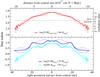 |
Fig. 13 Excitation- and ionization-sensitive line ratios. The dashed lines are the spectra along the slits through the center in original orientation (E-W) and the same spectrum reversed in direction to show the asymmetries. The thick lines are the average of both directions. The excitation class and level of separation of medium to high excitation is used according to the calibration by Reid & Parker (2010). |
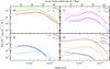 |
Fig. 14 Complete CLOUDY model of the main nebula. The dashed lines give the observational data, while the full lines depict the model. The spectral lines in the left panels a) and b) are used to fit the free parameters of the density law, the filling factor, and the temperature of the CSPN. The right panels c) and d) give the results derived for other lines from the best-fit model. The VLA intensities were arbitrarily scaled to the same level as the peak in Hα. |
Only the spatial profiles of [O iii] λ5007 Å, H α, He iλ4471 Å and He iiλ4686 Å were used to fit the free parameters of the nebula. For helium, the λ4471 Å line was used instead of the brighter λ5876 Å line, because it was covered by the significantly deeper ESO spectra. The fitting of the stellar temperature is completely dominated by the He i to He ii line ratio. The He ii to [O iii] ratio in the inner region can only be described with the CSPN model by Rauch et al. (1999). This suggests that the inner region is dominated by the products of the stellar winds from the current photosphere of the CSPN. All other abundances were taken from the intrinsic set for PNe in CLOUDY by Aller & Czyzak (1983) and Khromov (1989). There were not enough lines to derive detailed, spatially resolved abundances for other elements in this fitting procedure as free parameters. The best fit-model is summarized in Table 6.
After fitting the whole set of free parameters, all other detected lines in the spectra were calculated (Fig. 14, Table A.1). No iteration or feedback on the model was necessary. Even within the errors, no major deviations from the abundances seem to be required.
The simple model of the VLA data (see Fig. 14) was produced by using the free electrons of hydrogen and helium and assuming only free-free radiation. The radio flux density was scaled to the same level of peak as the H α line to fit into the scale of the plot. Additional it was smeared with a Gaussian, representing the beam size given by Taylor & Morris (1993). We also show in Fig. 14 that the feature around λ4712 Å cannot be described by [Ar iv]+He i. At the inner region of the hot wind bubble, a high-excitation species additionally seems to contribute to the wind. This region was not modeled in this setup. A possible candidate might be Ne iv, although the contribution calculated by CLOUDY lies a factor of 40 below the other two lines in the main nebula.
The resulting integrated mass of the main nebula model is 0.45 M⊙. This is a high, but still feasible mass for a PN.
Parameters of the best-fit model of the shell (38′′-72′′).
6.2. Shell
Because the electron density in the shell is about two orders of magnitude lower than that of the main nebula the sensitivity of the VLA observation was unfortunately insufficient to obtain a direct measurement, and diagnostic diagrams using forbidden lines saturate below ne ≈ 50...100 cm-3. Therefore we derived model calculations. Only the lines of H α, H β, [O iii] λ5007 Å and [N ii] λ6548 Å + λ6584 Å are sufficiently bright for the profile analysis. [O iii] λ4363 Å was detected close to the noise level. Accordingly, we used the average value of the electron temperature of 13 200 K (see Fig. 9) between 42′′ and 60′′ instead of a free input parameter of the fit.
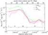 |
Fig. 15 CLOUDY model of the shell (dashed lines = observations, full lines = model). Because only a few lines could be used, it has the density and the filling factor as single free parameters (see text). The inner regions (I−III) are not fitted in this model, but taken from the main nebula model. |
The CLOUDY model of the shell (Fig. 15) uses the transmitted radiation of the main nebula model. It requires a density of nH ≈ 7...30 cm-3 (see Table 7). The H α/[N ii] line ratio is slightly higher than unity. This ratio can only be achieved by a filling factor higher than the one in the main nebula for this plasma. The calculations provide nearly the same results for the three lines in the whole range: 0.5≤ filling factor ≤1.0. Therefore we cannot conclude about this parameter.
6.3. Comparison with the RTH models
The radiative transfer hydrodynamic (RTH) models calculated for NGC 2438 by Corradi et al. (2000), Schönberner & Steffen (2002) and Perinotto et al. (2004) lead to different results in some aspects.
The results of a 1D RTH calculation by Corradi et al. (2000) and Schönberner & Steffen (2002) mainly show recombining gas in the shell. The electron number density is one order of magnitude lower than that of hydrogen. In the RTH models, a temperature of 2000 to 3000 K is indicated. So we tested various setups with fixed electron temperatures down to 2000 to 3000 K, but they did not result in a fit of the ratio of the observed lines at a reasonable density. Additionally, there is no detection of the [O i] lines (although these lines are affected by substraction of the Earth’s aurora). After applying estimates on the strengths and variation of the telluric lines by the methods described in Noll et al. (2012), we are quite confident about this result. The ratio predicted by the RTH models is [O i] λ 6300 Å : H β = 6:1, but we cannot confirm this result.
The resulting integrated mass of the main nebula model is 0.45 M⊙ in our calculations. It is about a factor of two higher than the mass calculated by Corradi et al. (2000), integrating the RTH model at their adopted distance of 1.0 kpc. At the recalculated distance of 1.9 kpc, their model gives a mass of 1.7 M⊙.
The resulting integrated mass of the shell is about 0.5 to 0.8 M⊙ in our determinations. The RTH models of Okorokov et al. (1985), Corradi et al. (2000) and Perinotto et al. (2004) assumed that the shell is AGB wind material. Calculations with such an AGB wind with a terminal velocity of 10 km s-1 and a typical mass-loss rate of 2.5 × 10⁻⁵M⊙ yr-1 result in a mass of 0.8 M⊙ in the same volume, consistent with our results. The different density used in the RTH models of Corradi et al. (2000) and Perinotto et al. (2004) leads to a very high mass estimate of 3.5 M⊙ at a distance of 1.9 kpc. This would require a very high mass-loss of ≳1.1 × 10⁻⁴M⊙ yr-1 during the late-AGB phase. At the smaller distance of 1 kpc, their calculations result in an integrated mass of about 0.5 M⊙. But such small distances are excluded (see Sect. 4).
The reason for the differences in the results may be found in the change of the input parameters (e.g., distance or luminosity). The RTH models used older input parameters in their calculations. Some of these parameters have changed owing to new measurements and calculations. An update of the RTH models to include the new measurements would be of interest to test whether the results would converge. The evidence for clumping may also complicate the interpretation of the 1D RTH models.
7. Conclusions
The observations of NGC 2438 allowed us to derive an individual distance of 1.9 ± 0.2 kpc and a foreground extinction of  . We confirm its non-membership of the open cluster M 46 in the foreground. The large discrepancy of the nebula luminosity and the CSPN luminosity (Rauch et al. 1999) is completely resolved with these values.
The model of the main nebula indicates that the old MSPN is matter bounded. The filling factor in the inner region is lower than that in the outer part of the main nebula. This is very similar to the observational results of the spatially resolved younger Ring Nebula and Helix Nebula. Although using only four lines in the parameter fitting, the photoionization model shows a nearly perfect representation of all observed lines. The analysis of the shock-sensitive tracers indicates that shocks do not contribute to the excitation of low-ionized atoms such as [N ii] and [S ii]. This old nebula is dominated by photoionization.
The surface brightness distribution of a few bright lines by the RTH models (Corradi et al. 2000; Perinotto et al. 2004) led to a fair representation of the whole nebula. However, the excitation and temperature throughout the nebula, and beyond, necessitates including small-scale clumps to obtain a self consistent model. A combination of the sophisticated hydrodynamical calculations in the RTH models, including effects of turbulence and clump formation with photoionization, is required for a complete view.
The determined temperature of the shell and the missing bright [O i] lines led us to conclude that the shell of NGC 2438 is fully ionized. Even the [O iii] lines indicate a photoionized state. Final confirmation by observations of shock-sensitive lines (e.g. [S ii] λ6716 Å/λ6732 Å) to verify possible other excitations is still lacking. More detailed investigations to derive electron temperatures from lower ionized species (e.g., [N ii](λ6548 Å + λ6584 Å)/[N ii]λ5755 Å or [O ii](λ3727 Å + λ3729 Å)/[O ii](λ7320 Å + λ7330 Å)) and from elements not influenced by depletion in dust grains, such as [Ar iii] λ5192 Å/(λ7135 Å + λ7751 Å), are highly desired for the main nebula out to the shell. As recently shown by Pilyugin et al. (2010), these line ratios can achieve very high accuracies. We also showed that the combination of these lines with H β can directly achieve abundances. Furthermore, a detailed investigation of the high-excitation features in the inner hot wind bubble and of the wind itself emerging from the CSPN is suggested. It is desired to complete the whole image and to give input to multi-dimensional radiative transfer hydrodynamic calculations.
Acknowledgments
We thank Thomas Rauch (Tübingen) for extensive discussions, help with the stellar atmosphere model for and providing us with the ESO 3.6 m (taken under proposal 64.H-0557) and SAAO 1.9 m data. We thank Greg Taylor (U. New Mexico) for providing the original FITS image of his VLA observations obtained under proposal AM0302. S.Ö. is supported by the Austrian Fonds zur Wissenschaftlichen Forschung, FWF doctoral school project W1227. The HST archival images were taken under Proposal 11827 (P.I. Keith Noll). This research has made use of the SIMBAD and Aladin data bases, operated at CDS, Strasbourg, France.
References
- Acker, A., Marcout, J., Ochsenbein, F., et al. 1992, The Strasbourg-ESO Catalogue of Galactic Planetary Nebulae Parts I, II (European Southern Observatory, Garching, Germany) [Google Scholar]
- Aller, L. H., & Czyzak, S. J. 1983, ApJS, 51, 211 [NASA ADS] [CrossRef] [Google Scholar]
- Armsdorfer, B., Kimeswenger, S., & Rauch, T. 2002, Rev. Mex. Astron. Astrofis. Conf. Ser., 12, 180 [Google Scholar]
- Armsdorfer, B., Kimeswenger, S., & Rauch, T. 2003, IAUS, 209, 511 [NASA ADS] [Google Scholar]
- Balick, B., Gonzalez, G., Frank, A., Jacoby, G. 1992, ApJ, 392, 582 [NASA ADS] [CrossRef] [Google Scholar]
- Bensby, T., & Lundstr"om, I. 2001, A&A, 374, 599 [NASA ADS] [CrossRef] [EDP Sciences] [Google Scholar]
- Blöcker, T. 1995, A&A, 297, 727 [NASA ADS] [Google Scholar]
- Chu, Y.-H., Jacoby, G. H., & Arendt, R. 1987, ApJS, 64, 529 [NASA ADS] [CrossRef] [Google Scholar]
- Colina, L., Bohlin, R. C., & Castelli, F. 1996, AJ, 112, 307 [NASA ADS] [CrossRef] [Google Scholar]
- Condon, J. J., Cotton, W. D., Greisen, E. W., et al. 1998, AJ, 115, 1693 [NASA ADS] [CrossRef] [Google Scholar]
- Copetti, M. V. F., & Writzl, B. C. 2002, A&A, 382, 282 [NASA ADS] [CrossRef] [EDP Sciences] [Google Scholar]
- Corradi, R. L. M., Schönberner, D., Steffen, M., & Perinotto, M. 2000, A&A, 354, 1071 [NASA ADS] [Google Scholar]
- Corradi, R. L. M., Schönberner, D., Steffen, M., & Perinotto, M. 2003, MNRAS, 340, 417 [NASA ADS] [CrossRef] [Google Scholar]
- Dalnodar, S., & Kimeswenger, S. 2011, Asymmetric Planetary Nebulae 5 Conf., eds. A.-A. Zilskra, F. Lykov, I. McDonald, & E. Lagadec, 81 [Google Scholar]
- Decin, L. 2012, AdSpR, 50, 843 [Google Scholar]
- Fluks, M., & The, P. 1992, A&A, 255, 477 [NASA ADS] [Google Scholar]
- Ferland, G. J., Korista, K. T., Verner, D. A., et al. 1998, PASP, 110, 761 [Google Scholar]
- Ferland, G. J., Porter, R. L., van Hoof, P. A. M. 2013, Rev. Mex. Astron. Astrofis., 49, 137 [Google Scholar]
- García Lario, P., Manchado, A., Riera, A., Mampaso, A., & Pottasch, S. R. 1991, A&A, 249, 223 [NASA ADS] [Google Scholar]
- Guerrero, M. A., & Manchado, A. 1999, ApJ, 522, 378 [NASA ADS] [CrossRef] [Google Scholar]
- Guerrero, M. A., Toalá, J. A., Medina, J. J., et al. 2013, A&A, 557, A121 [NASA ADS] [CrossRef] [EDP Sciences] [Google Scholar]
- Kaler, J. B. 1983, ApJ, 271, 188 [NASA ADS] [CrossRef] [Google Scholar]
- Kaler, J. B., Shaw, R. A., & Kwitter, K. B. 1990, ApJ, 359, 392 [NASA ADS] [CrossRef] [Google Scholar]
- Keenan, F. P., Kingston, A. E., & Johnson, C. T. 1988, A&A, 202, 253 [NASA ADS] [Google Scholar]
- Khromov, G. S. 1989, Space Sci. Rev., 51, 339 [NASA ADS] [CrossRef] [Google Scholar]
- Kingsburgh, R. L., & Barlow, M. J. 1994, MNRAS, 271, 257 [NASA ADS] [CrossRef] [Google Scholar]
- Kiss, L. L., Szabó, Gy. M., Balog, Z., Parker, Q. A., & Frew, D. J. 2008, MNRAS, 391, 399 [NASA ADS] [CrossRef] [Google Scholar]
- Magrini, L., Perinotto, M., Corradi, R. L. M., & Mampaso, A. 2003, A&A, 400, 511 [NASA ADS] [CrossRef] [EDP Sciences] [Google Scholar]
- Majaess, D., Turner, D., & Lane, D. 2007, PASP, 119, 1349 [NASA ADS] [CrossRef] [Google Scholar]
- Matsuura, M., Speck, A. K., McHunu, B. M., et al. 2009, ApJ, 700, 1067 [NASA ADS] [CrossRef] [Google Scholar]
- Meatheringham, S. J., Wood, P. R., & Faulkner, D. J. 1988, ApJ, 334, 862 [NASA ADS] [CrossRef] [Google Scholar]
- Mikołajewska, J., Brandi, E., Hack, W., et al. 1999, MNRAS, 305, 190 [NASA ADS] [CrossRef] [Google Scholar]
- Noll, S., Kausch, W., Barden, M., et al. 2012, A&A, 543, A92 [NASA ADS] [CrossRef] [EDP Sciences] [Google Scholar]
- O’Dell, C. R., Balick, B., Hajian, A. R., Henney, W. J., & Burkert, A. 2003, Rev. Mex. Astron. Astrofis. Ser. Conf., 15, 29 [NASA ADS] [Google Scholar]
- O’Dell, C. R., Henney, W. J., & Ferland, G. J. 2005, AJ, 130, 172 [NASA ADS] [CrossRef] [Google Scholar]
- Okorokov, V. A., Shustov, B. M., Tutukov, A. V., & Yorke, H. W. 1985, A&A, 142, 441 [NASA ADS] [Google Scholar]
- Osterbrock, D. E., & Ferland, G. J. 2006, Astrophysics of gaseous Nebulae and active Galactic Nuclei (Sausalito: University Science Books) [Google Scholar]
- Paunzen, E., Heiter, U., Netopil, M., & Soubiran, C. 2010, A&A, 517, A32 [NASA ADS] [CrossRef] [EDP Sciences] [Google Scholar]
- Perinotto, M., Schönberner, D., Steffen, M., & Calonaci, C. 2004, A&A, 414, 993 [NASA ADS] [CrossRef] [EDP Sciences] [Google Scholar]
- Phillips, J. P. 2004, Rev. Mex. Astron. Astrofis., 40, 193 [NASA ADS] [Google Scholar]
- Pilyugin, L. S., Vílchez, J. M., & Thuan, T. X. 2010, ApJ, 720, 1738 [NASA ADS] [CrossRef] [Google Scholar]
- Proxauf, B., Öttl, S., & Kimeswenger, S. 2014, A&A, 561, A10 [NASA ADS] [CrossRef] [EDP Sciences] [Google Scholar]
- Ramos-Larios, G., & Phillips, J. P. 2012, MNRAS, 425, 1091 [NASA ADS] [CrossRef] [Google Scholar]
- Ramos-Larios, G., Vázquez, R., Guerrero, M. A., et al. 2012a, MNRAS, 423, 3753 [NASA ADS] [CrossRef] [Google Scholar]
- Ramos-Larios, G., Guerrero, M. A., Vázquez, R., & Phillips, J. P. 2012b, MNRAS, 420, 1977 [NASA ADS] [CrossRef] [Google Scholar]
- Rauch, T. 2003, IAUS, 209, 191 [NASA ADS] [Google Scholar]
- Rauch, T., Köppen, J., Napiwotzki, R., & Werner, K. 1999, A&A, 347, 169 [NASA ADS] [Google Scholar]
- Reid, W. A., & Parker, Q. A. 2010, PASA, 27, 187 [NASA ADS] [CrossRef] [Google Scholar]
- Ringat, E. 2012, ASP Conf. Ser., 452, 99 [NASA ADS] [Google Scholar]
- Schmeja, S., & Kimeswenger, S. 2001, A&A, 377, L18 [NASA ADS] [CrossRef] [EDP Sciences] [Google Scholar]
- Schneider, S. E., & Buckley, D. 1996, ApJ, 459, 606 [NASA ADS] [CrossRef] [Google Scholar]
- Schönberner, D., & Steffen, M. 2002, Rev. Mex. Astron. Astrofis., 12, 144 [Google Scholar]
- Sharma, S., Pandey, A. K., Ogura, K., et al. 2006, AJ, 132, 1669 [NASA ADS] [CrossRef] [Google Scholar]
- Speck, A. K., Meixner, M., Jacoby, G. H., & Knezek, P. M. 2003, PASP, 115, 170 [NASA ADS] [CrossRef] [Google Scholar]
- Stanghellini, L., & Kaler, J. B. 1989, ApJ, 343, 811 [NASA ADS] [CrossRef] [Google Scholar]
- Taylor, G. B., & Morris, A. 1993, ApJ, 409, 720 [NASA ADS] [CrossRef] [Google Scholar]
- Torres-Peimbert, S., & Peimbert, M. 1977, Rev. Mex. Astron. Astrofis., 2, 181 [NASA ADS] [Google Scholar]
- van de Steene, G. C., & Zijlstra, A. A. 1995, A&A, 293, 541 [NASA ADS] [Google Scholar]
- Vicini, B., Natta, A., Marconi, A., et al. 1999, A&A, 342, 823 [NASA ADS] [Google Scholar]
- Vollmer, B., Gassmann, B., Derrière, S., et al. 2010, A&A, 511, A53 [NASA ADS] [CrossRef] [EDP Sciences] [Google Scholar]
- Warmels, R. H. 1991, PASP Conf. Ser., 25, 115 [NASA ADS] [Google Scholar]
- Zhang, Y., Hsia, C.-H., & Kwok, S. 2012, ApJ, 755, 53 [NASA ADS] [CrossRef] [Google Scholar]
- Zijlstra, A. A., Pottasch, S. R., & Bignell, C. 1989, A&AS, 79, 329 [NASA ADS] [Google Scholar]
Appendix A: Model results for the main nebula
The table gives the full best-fit model. The normalization on the left-hand side is relative to H β at each column individually. This allows viewing the line ratios in the way they are commonly used in nebular spectroscopy. The right-hand side table is normalized to H β only in the middle column to provide a better view on the radial evolution of individual line fluxes.
Measured line intensities vs. model lines of the best fit model of the main nebula.
All Tables
Parameters of the target and of the best-fit model of the main nebula (14′′−38′′).
Measured line intensities vs. model lines of the best fit model of the main nebula.
All Figures
|
Fig. 1 Overview of the target observations. The background image is an H α EFOSC1 image. The spectrograph slits were all positioned in the E-W direction. The SAAO slit numbers correspond to those in Table 1. The CSPN and the region names as defined in Sect. 1 are shown and the field of view of the HST WFPC2 images is indicated as well. |
| In the text | |
|
Fig. 2 Direct images of the main nebula. First row: He ii (λ4686 Å) and [O iii] (λ5007 Å); second row: VLA (20 cm) and H α (λ6563 Å) +[N ii] (λ6548 Å+λ6584 Å) (same orientation as shown in Fig. 1− N is up, E is left). The ellipses are derived from the images of the He ii line. While the He ii emission is clearly concentrated towards the inner edge of the main nebula, the [O iii] and VLA images have about the same appearance. |
| In the text | |
|
Fig. 3 HST images of the main nebula. First row: [O iii](λ5007 Å) and H α after subtracting [NII] contribution (see text); second row: [N ii] (λ6584 Å) and [S ii](λ6716 Å+λ6732 Å). The images are in the same orientation as shown in Fig. 1 and cover the field of view shown there. The similarities in the structures are obvious. |
| In the text | |
|
Fig. 4 Zoom of the N-E region of the main nebula from the HST images. The cometary knots are especially pronounced in the [O iii] images. The shadows point exactly away from the CSPN (direction indicated by two lines). |
| In the text | |
|
Fig. 5 The spatial distribution of the line ratio R = Hα/Hβ to search for intrinsic extinction. To cover homogeneous S/N ratios, a threshold of 3.5× below the S/N peak was chosen. Also the region around the CSPN was excluded. For the shell, the same procedure was applied, but 20× fainter. |
| In the text | |
|
Fig. 6 CSPN (thin black line) without removing the nebula emission lines, and the standard star EG 274 overlayed (smooth red line − scaled and the extinction |
| In the text | |
|
Fig. 7 Various lines of the nebula (logarithmic representation). The different spectral regions originate from different spectra (ESO and SAAO) and thus vary in S/N ratio at similar physical intensities. The panels show the excitation groups (criteria see text). The high-excitation species (upper panel) concentrate at the central region. The medium-excitation species (middle panel) smoothly follow the total brightness and the radial behavior of the VLA image throughout the nebula. The low-excitation species (lower panel) are dominated by clumpy structures. The O ii λ3729 is at the edge of the CCD and its flux calibration is very uncertain. It is added only for comparison of the profiles. |
| In the text | |
|
Fig. 8 Density derived from [S ii], in E-W direction through the CSPN. The line ratio (upper panel) and the electron density is nearly constant. The density profile does not follow the strong surface brightness variations (lower panel). |
| In the text | |
|
Fig. 9 Intensity (upper panel) of the [O iii] λ5007 Å, and the electron temperature using [O iii] (λ4958 Å+λ5007 Å)/λ4363 Å ratios along the slit (lower panel). The logarithmic scale is used to show the shell and the even farther extended halo. The flux scale is the same as in Fig. 7. The plus signs indicate the solution by exponential formula of Osterbrock & Ferland (2006). The bars give the solution using the new calibration of Proxauf et al. (2014). |
| In the text | |
|
Fig. 10 Diagnostic diagram of the separation of shocked nebulae from photoionized PNe (after Magrini et al. 2003). The points follow the sequence of the ionization class toward the center. The dashed line gives a fit through the good data points (filled symbols). No dependency on increase or decrease of the intensity can be found (small panel). |
| In the text | |
|
Fig. 11 log (Hα/ [N ii] ) − log (Hα/ [N ii]) image obtained from the HST frames. It is based on the same analysis as in Fig. 10. The expected value should be the same as the incline (0.7−0.8) of the trendline through the data points in Fig. 10. |
| In the text | |
|
Fig. 12 [O iii]/H α image from the HST data. No sudden changes in the line ratio are found. |
| In the text | |
|
Fig. 13 Excitation- and ionization-sensitive line ratios. The dashed lines are the spectra along the slits through the center in original orientation (E-W) and the same spectrum reversed in direction to show the asymmetries. The thick lines are the average of both directions. The excitation class and level of separation of medium to high excitation is used according to the calibration by Reid & Parker (2010). |
| In the text | |
|
Fig. 14 Complete CLOUDY model of the main nebula. The dashed lines give the observational data, while the full lines depict the model. The spectral lines in the left panels a) and b) are used to fit the free parameters of the density law, the filling factor, and the temperature of the CSPN. The right panels c) and d) give the results derived for other lines from the best-fit model. The VLA intensities were arbitrarily scaled to the same level as the peak in Hα. |
| In the text | |
|
Fig. 15 CLOUDY model of the shell (dashed lines = observations, full lines = model). Because only a few lines could be used, it has the density and the filling factor as single free parameters (see text). The inner regions (I−III) are not fitted in this model, but taken from the main nebula model. |
| In the text | |
Current usage metrics show cumulative count of Article Views (full-text article views including HTML views, PDF and ePub downloads, according to the available data) and Abstracts Views on Vision4Press platform.
Data correspond to usage on the plateform after 2015. The current usage metrics is available 48-96 hours after online publication and is updated daily on week days.
Initial download of the metrics may take a while.