| Issue |
A&A
Volume 565, May 2014
|
|
|---|---|---|
| Article Number | A120 | |
| Number of page(s) | 15 | |
| Section | Cosmology (including clusters of galaxies) | |
| DOI | https://doi.org/10.1051/0004-6361/201323077 | |
| Published online | 21 May 2014 | |
JKCS 041: a Coma cluster progenitor at z = 1.803
1 INAF − Osservatorio Astronomico di Brera, via Brera 28, 20121 Milano, Italy
e-mail: This email address is being protected from spambots. You need JavaScript enabled to view it.
2 Cahill Center for Astronomy and Astrophysics, California Institute of Technology, MS 249-17, Pasadena CA 91125, USA
3 Current Address: The Observatories of the Carnegie Institution for Science, 813 Santa Barbara St., Pasadena CA 91101, USA
4 Current Address: GEPI, Observatoire de Paris, 77 av. Denfert Rochereau, 75014 Paris, France
5 Department of Physics, University of California, Santa Barbara CA 93106, USA
Received: 18 November 2013
Accepted: 3 May 2014
Abstract
Using deep two-color near-infrared HST imaging and unbiased grism spectroscopy, we present a detailed study of the z = 1.803 JKCS 041 cluster. We confirm, for the first time for a high-redshift cluster, a mass of log M ≳ 14.2 in solar units using four different techniques based on the X-ray temperature, the X-ray luminosity, the gas mass, and the cluster richness. JKCS 041 is thus a progenitor of a local system like the Coma cluster. Our rich dataset and the abundant population of 14 spectroscopically confirmed red-sequence galaxies allows us to explore the past star formation history of this system in unprecedented detail. Our most interesting result is a prominent red sequence down to stellar masses as low as log M/M⊙ = 9.8, corresponding to a mass range of 2 dex. These quiescent galaxies are concentrated around the cluster center with a core radius of 330 kpc. There are only few blue members and avoid the cluster center. In JKCS 041 quenching was therefore largely completed by a look-back time of 10 Gyr, and we can constrain the epoch at which this occurred via spectroscopic age-dating of the individual galaxies. Most galaxies were quenched about 1.1 Gyr prior to the epoch of observation. The less-massive quiescent galaxies are somewhat younger, corresponding to a decrease in age of 650 Myr per mass dex, but the scatter in age at fixed mass is only 380 Myr (at log M/M⊙ = 11). There is no evidence for multiple epochs of star formation across galaxies. The size–mass relation of quiescent galaxies in JKCS 041 is consistent with that observed for local clusters within our uncertainties, and we place an upper limit of 0.4 dex on size growth at fixed stellar mass (95% confidence). Comparing our data on JKCS 041 with 41 clusters at lower redshift, we find that the form of the mass function of red sequence galaxies has hardly evolved in the past 10 Gyr, both in terms of its faint-end slope and characteristic mass. Despite observing JKCS 041 soon after its quenching and the three-fold expected increase in mass in the next 10 Gyr, it is already remarkably similar to present-day clusters.
Key words: galaxies: clusters: individual: JKCS041 / galaxies: clusters: general / galaxies: elliptical and lenticular, cD / galaxies: evolution / methods: statistical
© ESO, 2014
1. Introduction
It has been recognized for many years that clusters of galaxies are valuable laboratories for probing galaxy formation and evolution. The tightness of the red sequence of member galaxies implies a uniformly old age for their stellar populations (e.g., Bower et al. 1992; Stanford et al. 1998; Kodama & Arimoto 1997) which, together with the morphology-density relation (e.g., Dressler 1980), leads to two important conclusions: first, present-day clusters are the descendants of the largest mass fluctuations in the early Universe where evolutionary processes were accelerated; and second, cluster-specific phenomena, such as ram-pressure stripping or strangulation (e.g., Treu et al. 2003) played an important role in quenching early star formation.
Even though much can be inferred from the fossil evidence provided by studies of galaxies in local clusters, these are rapidly evolving systems and it is important to complement this information with studies of the galaxy population at the highest redshifts. The relevant observables include the location and width of the red sequence of quiescent members, the mass distribution along the sequence and the various trends such as the size–mass and the age–mass relations. Theoretical predictions of these observables are challenging because it is currently difficult to resolve star-forming regions in simulations that are sufficiently large to include representative rich clusters. Semi-analytic models do not suffer from such limitations but rely on simplifying assumptions (e.g., on the importance of merger-induced bursts and stellar feedback) and tunable recipes. Even worse, because clusters are complex environments, there is not always unambiguous insight into the relative importance of the different physical processes, which means that it is unclear which of them should be modeled.
For these reasons, a phenomenological approach is very productive and represents the route followed by many researchers. They have observed clusters progressively more distant to approach the epoch at which star formation was quenched and, particularly, to determine the various processes involved. Quenching is thought to occur at z ≲ 2 by some semi-analytic models (e.g., Menci et al. 2008) and it is observationally at z ≳ 1.2: since at z ≃1.2, the cluster population is largely evolving passively (e.g., de Propris et al. 1999), the red sequence is already in place at the highest redshift (z = 1.4, e.g., Stanford et al. 1998; Kodama & Arimoto 1997), and the processes responsible for truncating residual star formation are more effective in denser environments and for more massive galaxies (e.g., Raichoor & Andreon 2012b).
Beyond z ≃ 1.4, our knowledge of the properties of galaxy populations in clusters becomes incomplete. There is a paucity of clusters with reliable masses, spectroscopically confirmed members, and adequately deep imaging and spectroscopic data essential for determining past star formation histories (SFHs). The challenges of the complexity of astronomical data and the associated statistical analysis compound the paucity of the data. All this has led to some disagreement, for example, on the mass-dependent distribution of the passive population (cf. Mancone et al. 2010, 2012; Fassbender et al. 2011 vs. Andreon 2013; Strazzullo et al. 2010) and whether the color-density relation reverses from its local trends at high redshift (Tran et al. 2010 vs. Quadri et al. 2012).
We present a comprehensive analysis of the galaxies in the rich cluster JKCS 041, which was first identified by Andreon et al (2009). In a previous paper in this series (Newman et al. 2013, hereafter Paper I), we derived a redshift of z = 1.803 using HST grism spectroscopy, based on 19 confirmed members, a high proportion of which are quiescent. In the present paper we derive the mass of this cluster and examine the extent of the red sequence in the context of its likely subsequent evolution. By considering the color–magnitude relation, the age–mass relation and the spatial distribution of passive members, we argue that JKCS 041 can be regarded as the progenitor of a present-day Coma-like cluster.
The plan of the paper is as follow: in Sect. 2 we briefly review the HST data; details are available in Paper I. In Sect. 3 we estimate the mass of JKCS 041 using various diagnostics, including its X-ray properties and optical richness and compare these with those of other high-redshift clusters. In Sect. 4 we analyze the ages and colors of the passive members in detail, demonstrating an important result: the red sequence is fully populated down to low stellar masses. We also examine the age–mass relation and the spatial distribution of red members in light of conflicting results presented for other clusters. In Sect. 5 we discuss our results on JKCS 041 in the context of a sample of other clusters at lower redshift and consider the most likely evolutionary picture. We discuss the implications in Sect. 6.
Throughout this paper, we assume ΩM = 0.3, ΩΛ = 0.7, and H0 = 70 km s-1 Mpc-1. Magnitudes are in the AB system. We use the 2003 version of Bruzual & Charlot (2003, BC03 hereafter) stellar population synthesis models with solar metallicity and a Salpeter initial mass function (IMF). We define stellar masses as the integral of the star formation rate, and they therefore include the mass of gas processed by stars and returned to the interstellar medium. In Sects. 4.4 and 4.5, for consistency with Paper I, we instead use stellar masses that count only the mass in stars and their remnants; these masses are systematically lower by 0.12 dex.
2. Data
The primary data used in this paper were derived from the HST imaging and spectroscopic campaign (GO: 12927, PI: Newman) discussed in Paper I. Only a brief summary is provided, and we refer to Paper I for more details.
The imaging data consist of photometry in two bands, F105W (for a total observing time of 2.7 ks) and F160W (4.5 ks), denoted Y and H, respectively, derived using the SExtractor code (Bertin & Arnouts 1996). Total galaxy magnitudes refer to isophotal-corrected magnitudes, while colors are based on a fixed 0.5 arcsec diameter aperture, which is well suited for faint galaxies at the cluster redshift. The photometric data for red-sequence galaxies in the cluster is complete to Y = 26.6 mag (see Fig. 1). As a control sample (to estimate the number of back/foregound galaxies), we selected an area of 29.78 arcmin2 in the GOODS South area observed in a similar manner as part of the CANDELS program (GO: 12444/5, PI: Ferguson, Riess & Faber, Grogin et al. 2011; Koekemoer et al. 2011; we used the images distributed in Guo et al. 2013).
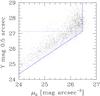 |
Fig. 1 Completeness of our Y-band imaging of JKCS 041. The Y-band magnitude within a 0.5 arcsec aperture compared with the peak surface brightness. There are galaxies with a peak surface brightness fainter than the detection threshold (~26.5 mag arcsec-2, vertical line), but they are undetectable with these data. Extrapolating the trend seen at brighter magnitudes (slanted solid line), the completeness limit (horizontal dashed line) is 27.15 mag. Owing to uncertainties inherent in this extrapolation, we conservatively adopt a limit that is 0.5 mag brighter, which leads to a limiting magnitude of Y = 26.6. |
The spectroscopic data were taken with the WFC3/IR G102 and G141 grisms at three epochs (and hence orientations) to reduce contamination. The spectra sample from 3000 to 6000 Å in the rest-frame of galaxies at z = 1.8. Redshifts were published in Paper I for 63 emission-line galaxies brighter than H = 25.5 mag and 35 absorption-lines galaxies brighter than H = 23.3 mag. Nineteen of these are cluster members. The absorption-line galaxy sample of Paper I has a pre-selection based on photometric redshift estimates, such that only galaxies with 1.4 <zphot< 3 were considered; no such cut was applied for emission-line galaxies.
For this paper and for the purpose of checking completeness, we also extracted and fit the spectra of those few bright (H< 22.5 mag) galaxies irrespective of their photo-z within 1.22 times the area enclosed by the outermost detected X-ray isophote (1.8 arcmin2, about 0.5 Mpc2). These targets were not considered in Paper I. The successfully extracted spectra indicate redshifts z< 1.2, in agreement with the photo-z pre-selection. Of the four unsuccessfully extracted spectra, two represent galaxies that are very likely too extended to be at high redshift. The two remaining galaxies have a low photo-z and are probably foreground galaxies. Therefore, the sample of galaxies with H< 22.5 mag with spectroscopic redshifts represents a complete sample of cluster members.
In this paper we complement the HST data with data from the WIRCam Deep Survey (WIRDS) survey (Bielby et al. 2012), which enables us to estimate the mass of JKCS 041 from its richness (see Sect. 3). WIRDS provides deep z′ and J photometry of a 1 deg2 field around JKCS 041 to a limit of z′ = 25 mag. Our earlier papers characterized the red-sequence relation for JKCS 041 on the basis of these data (Andreon 2011; Raichoor & Andreon 2012a).
3. Mass of the JKCS 041 cluster
We now turn to the mass of JKCS 041 which can be estimated in four ways.
-
1.
Using the X-ray temperature-mass relation under theassumption that the locally determined relation evolvesself-similarly. Although this assumption has been challenged by,for example, Andreon et al. (2011 and referencestherein), the implications are not yet precisely quantified giventhat samples with a known selection function would be required(Pacaud et al. 2007; Andreon et al.2011; Maughan et al. 2012).
-
2.
Using the LX-mass relation (Vikhlinin et al. 2009), again assuming a self-similar-inspired evolution.
-
3.
Using the gas mass, assuming that the gas fraction has not changed in the past 10 Gyr.
-
4.
Using a local richness-mass relation (e.g., Johnston et al. 2007; Andreon & Hurn 2010). The mass estimated from the cluster richness is probably relatively independent of evolutionary effects, given that the color evolution of red members is reasonably well understood (e.g., De Propris et al. 1999, see also Sect. 5.1).
For the first three methods we used the results from the Chandra observations reported by Andreon et al. (2009), rescaled to the current redshift and to the same aperture r200 assuming a Navarro et al. (1997) profile of concentration 3 − 5. We find log M200/M⊙ = 14.6 ± 0.5 from the X-ray temperature. Using the X-ray luminosity in the [0.5−2] keV band within r500 and the Vikhlinin et al. (2009) calibration, we find log M200/M⊙ ≈ 14.45. For this latter estimate, there is an uncertainty of ≥0.2 dex, mostly arising from the scatter in LX at a given mass (Vikhlinin et al. 2009, ≥0.11 dex) with 0.08 dex arising from uncertainties in the count rate and temperature. Assuming a 10 % gas fraction, typical of nearby clusters (Vikhlinin et al. 2009), we find log M200/M⊙ ≈ 14.4 from the gas mass within r500 (Ettori et al. 2004). This gas-based mass has an error of ≥0.10 dex, derived from a 0.08 dex arising from the uncertainties in the gas-mass profile and the local Universe ~0.06 dex scatter of the gas fraction (Andreon 2010), to which we need to add an unknown uncertainty because of the evolution of the gas fraction. Adopting the Universe baryon fraction as value of the gas fraction, we find log M200/M⊙ ≈ 14.2. Given that it is unlikely that the gas fraction exceeds the Universe baryon fraction, at face value log M200/M⊙ ≈ 14.2 is a reasonable lower limit of the JKCS 041 mass. Finally, from the X-ray profile and spectrum normalization, we computed a gas mass within 30 arcsec of 3.9 × 10¹² M⊙, fully consistent with the upper limit derived from SZ observations in Culverhouse et al. (2010) and extrapolation of lower redshift scaling relations.
The fourth method uses the large area sampled by the WIRDS images and, using the calibration of Andreon & Hurn (2010), is based on the number of red-sequence galaxies brighter than  mag within r200, correcting for line-of-sight contamination using galaxies at projected radii 6.5 <r< 9.1 Mpc. To derive the equivalent local luminosity
  , we assumed passive evolution using the BC03 models with a simple stellar population formed at redshift zf = 3, a Salpeter IMF and solar metallicity, although the results are not sensitive to these parameters. With 20 red-sequence galaxies brighter than Ks = 21.99 mag within 1.43 Mpc, JKCS 041 is within the lower half of the mass range 13.7 < log M/M⊙< 15 discussed by Andreon & Hurn (2010). Using their Eq. (18), we estimate r200 = 0.76 Mpc, which contains 17 members, and derive log M200/M⊙ = 14.25 ± 0.29. This uncertainty takes into account the intrinsic scatter in mass at a given richness (the dominating term), the limited number of members, and the uncertainty of the calibrating relation.
As can be seen, the richness-based mass estimate agrees reasonably well with the mass estimates: log M200/M⊙ = 14.6 ± 0.5 from the X-ray temperature, log M200/M⊙ ≈ 14.45 from the X-ray luminosity, and log M200/M⊙ ≈ 14.4 from the gas mass. This is a unique achievement for such a high-redshift cluster. All four determinations agree to better than 1 combined standard deviation, indicating that JKCS 041 is an intermediate-mass cluster by the standards of local systems, and a massive cluster at such high redshift. In fact, a typical z = 1.8 cluster with log M200/M⊙ ≈ 14.25 will grow in mass (Fakouri et al. 2010) to become a log M200/M⊙ ≈ 14.75 cluster locally, albeit with an uncertainty due to the stochastic nature of the mass growth in a hierarchical Universe. Nonetheless, our mass estimates suggest that JKCS 041 is a credible ancestor of a present-day, Coma-like cluster.
3.1. Comparing JKCS 041 with other high-redshift clusters
In light of these results, we now compare the mass of the JKCS 041 cluster with that of other high-redshift systems in the literature.
Following the same method and local calibration as used for JKCS 041, Stanford et al. (2012) derived a mass of log M200/M⊙ ≈ 14.5 ± 0.1 from LX for IDCS J1426.5+3508 (z = 1.75), similar to the value derived for JKCS 041, but with a smaller uncertainty, because the authors determined it on statistical measurement errors alone. Given that both clusters are at similar redshift, a comparison of the X-ray luminosities obtained in comparable apertures is illustrative. As neither the X-ray temperature nor the X-ray surface brightness radial profile is measurable for IDCS J1426.5+3508, we can only compare the X-ray count rates in similar apertures (1 arcmin for both clusters). We found a factor two in count rate, which, divided by the slope of the LX-mass relation (1.6), gives a factor 1.5 in mass, with IDCS J1426.5+3508 being more massive. However, allowing for the scatter in LX at a given mass, the masses of the two clusters are statistically indistinguishable.
To compare the mass estimate based on richness, we also need to compare the relative fraction of red galaxies. Since both clusters have similar richness within 1 arcmin (Andreon 2013), their masses are also expected to be similar. We note, however, that while the bright galaxies in JKCS 041 are all red (Raichoor & Andreon 2012; Andreon 2013 and Sect. 4.1), there are several blue galaxies in IDCS J1426.5+3508 (see Andreon 2013), indicating a lower richness n200. Inspection of the color–magnitude relation of the two clusters reinforces this impression: while all bright galaxies are on the red sequence in JKCS 041, the red sequence of IDCS J1426.5+3508 seems poorly populated, and even more so if some allowance is made for background/foreground contamination (the almost totality of red sequence IDCS J1426.5+3508 galaxies has an unknown membership).
By contrast, the CL J1449+0856 structure at z = 1.99 (Gobat et al. 2009) has a much lower mass. Only the brightest cluster member is more luminous than mag. Because of the paucity of luminous members for CL J1449+0856, there are no low-redshift structures in the sample of Andreon & Hurn (2010), which we may use as a calibrator, except for possibly the NGC4325 group, with two galaxies brighter than mag and mass log M200/M⊙ = 13.3 ± 0.3. This value is lower than, although formally consistent with, that estimated by Gobat et al. (2011) using LX and the estimate from Strazzullo et al. (2013) derived from the total stellar mass within r500 (using the local calibration of Andreon 2012). Both estimates indicate a mass an order of magnitude lower that JKCS 041 and IDCS JKCS 0411426.5+3508, consistent with its smaller core radius (20 kpc, Strazzullo et al. 2013).
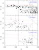 |
Fig. 2 Color−magnitude diagram. Upper panel: JKCS 041 spectroscopic members (solid dots) and all 22.5 <H galaxies within the JKCS 041 area (open dots). The locus of an SSP with zf = 5,3,2.5 is shown for comparison (solid lines, from top to bottom). For clarity, error bars are only shown for Y − H> 1 mag galaxies. Central panel: spectroscopic non-members. Bottom panel: control field galaxies with 22.5 <H< 25 mag. In all panels the JKCS 041 Y-band completeness limit is indicated with a slanted dashed line (Y = 26.6 mag), along with the corresponding H completeness limit (vertical dashed line, H = 25 mag) for the reddest red-sequence galaxies. The JKCS 041 spectroscopic completeness limit of H = 22.5 and the locus of red-sequence galaxies (red dashed corridor) are also shown. |
4. The galaxy population of JKCS 041
4.1. A fully-populated red sequence
In this section we isolate the red-sequence members of JKCS 041 and show, for the first time in a high-redshift cluster, the presence of quenched galaxies over a 2 dex range in stellar mass at a look-back time corresponding to only 3.5 Gyr after the Big Bang.
As described earlier, our catalog is spectroscopically complete for galaxies with H< 22.5 mag that lie within the outermost detected X-ray isophote enlarged by a factor of 1.21. For these bright galaxies, we have proof of membership for each galaxy. For fainter galaxies with 22.5 <H< 25 mag, however, we must statistically estimate the contamination by galaxies unrelated to the cluster using the GOODS-S control field.
The top panel of Fig. 2 shows all galaxies within this area that are either confirmed spectroscopic members (15, solid points) or whose membership is unknown (open circles). Additionally, we plot the four remaining spectroscopic members found outside this area (two are red and two are blue). The figure demonstrates that at H< 22.5 mag, all members are red galaxies, in agreement with previous results based on a purely statistical analysis of membership (Andreon & Huertas-Company 2011; Raichoor & Andreon 2012a). We detected in our Chandra data one red-sequence member (LX ≈ 6 × 1042 erg s-1 [0.5, 2] keV) that might accomodate a low luminosity AGN. No other members are detected, and for them we derive LX< 1043 erg s-1. None of the red-sequence galaxies, nor their stack were detected in the SWIRE data (Paper I). The red sequence is much more prominent than other high-redshift clusters, in particular the z = 1.75 cluster IDCS J1426.5+3508 (Stanford et al. 2012). The Y − H color of the JKCS 041 red sequence is consistent with expectations for a simple stellar population (SSP) formed at zf = 2.5 − 3.0, based on BC03 models with a Salpeter IMF and solar metallicity2. Most of the spectroscopic non-members, shown in the middle panel, are bluer than the cluster red sequence. Many of the red non-members are also at high redshift, but do not meet the membership criterion defined in Paper I (| z − zclus | < 0.022).
The bottom panel of Fig. 2 compares the color distribution in the GOODS-S control field. Although this field covers 29.78 arcmin2, for clarity we only show galaxies drawn from a solid angle equal to the cluster field. The comparison reveals more galaxies with Y − H ~ 1.3 mag in the cluster, indicating that the cluster red sequence is very well defined at all luminosities: at the bright end, where we were able to eliminate non-members using grism spectroscopy, and at the fainter end, where it is evident to H = 25 mag. This is the first time that the red sequence has been traced in clusters to such luminosities at high redshift, which is due to the depth of our Y-band observations.
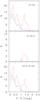 |
Fig. 3 Color distribution in the cluster (red) and control field (blue) for all galaxies (top panel), bright galaxies (middle panel) and faint galaxies (bottom panel). Since membership is available on an individual basis for the bright galaxies, no control field is required for the middle panel. Colors are corrected for the slope of the color−magnitude relation assuming a slope of 0.05, consistent with the JKCS 041 data and with slopes observed at z = 0. |
More quantitatively, Fig. 3 shows the color distribution in the cluster and control fields (red and blue lines, respectively) for the entire sample (H< 25 mag) and for two subsamples divided at H = 22.5 mag. All colors are corrected for the color–magnitude slope. Since spectroscopic membership is known for bright galaxies, background contamination is not an issue for H< 22.5 mag. The data reveal a clear excess of galaxies at Y − H ~ 1−1.7 mag in both the brighter and fainter subsamples. This excess (28 galaxies) far exceeds the observed scatter in our control field across regions of JKCS 041 solid angle and expectations from cosmic variance (Moster et al. 2011). The slope-corrected 1 <Y − H< 1.7 mag range is our working definition of red-sequence galaxies. With this definition one spectroscopic member (ID447) brighter than H = 22.5 mag is blue (by a small margin, 0.02 mag), as are three fainter galaxies (693, 531, 332). These latter systems were classified as star-forming in Paper I on the basis of their UVJ colors, and the two bluest show emission lines in their spectra.
Figure 3 also shows an excess of bluer galaxies (Y − H< 1 mag) galaxies in the direction of JKCS 041. Some of these are most likely members of JKCS 041 (including the three spectroscopically-confirmed blue members), while the others belong to structures along the line of sight. The area around JKCS 041 is known to contain several foreground groups and structures (Le Fevre et al. 2005; Andreon et al. 2009; Andreon & Huertas-Company 2011 and Paper I). These excess blue galaxies are therefore expected and are not relevant for the remainder of this paper, which is focused on the red cluster members.
In summary, the red sequence of JKCS 041 is populated over an unprecedented 5 mag in luminosity, indicating that quenching was already effective 10 Gyr ago. Because semi-analytic models (e.g., Menci et al. 2008) predict a depopulated red sequence at bright magnitudes, our observations indicate that the epoch of quenching may be earlier than these models assume. Similarly, McGee et al. (2009) predicted that environmental quenching is negligible by z ~ 1.5, while our comparison between JKCS 041 and the z ~ 1.8 field population clearly shows that environmental processes are responsible for quenching more than half of the cluster members (Paper I, Fig. 8).
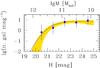 |
Fig. 4 Luminosity (bottom axis) and stellar mass (top axis) function of red-sequence cluster members. The solid line is the mean model fitted to the individual galaxy data, while the shading indicates the 68% uncertainty (highest posterior density interval). Points and approximated error bars are derived by binning galaxies in magnitude bins, adopting approximated Poisson errors summed in quadrature, as commonly done in the literature. The top axis indicates the corresponding stellar mass, based on our standard BC03 SSP model with zf = 3. |
4.2. The mass function of JKCS 041
The stellar mass function (MF) represents the zeroeth-order statistic of a galaxy sample, giving the relative number of member galaxies as a function of their mass.
Figure 4 shows the mass function of red-sequence galaxies in JKCS 041 with log M/M⊙> 9.8. (As in Sect. 4.1, we considered galaxies located within the outermost X-ray isophote enlarged by a factor of 1.2). Here we converted the observed H-band luminosity to stellar mass assuming our standard BC03 SSP model with zf = 3. After accounting for the different mass definitions (Sect. 1), masses derived from this procedure are consistent with those derived from fits to the grism spectroscopy and 12-band photometry (Paper I): the median difference and interquartile range are 0.02 dex and 0.10 dex, respectively, for red-sequence galaxies.
The luminosity function (LF) was derived by fitting a Schechter (1976) function (for the cluster galaxies) by statistically subtracting the field population for 22.5 <H< 25, whose log abundance was taken to be linear. The relevant likelihood expression was taken from Andreon et al. (2005), which is an extension of the Sandage et al. (1979) likelihood when a background component is present. Uniform priors were taken for the five parameters. For display purposes, we also computed approximate LFs, by binning galaxies in magnitude and adopting approximated errors as usual (e.g., Zwicky 1957; Oemler 1974). These approximate LFs are plotted in the figures as points with error bars, although the fit itself is based on the unbinned data.
For the JKCS 041 red sequence, we derive a characteristic magnitude H∗ = 21.6 ± 0.5 mag, a characteristic mass log M/M⊙ ~ 11.2, a faint-end slope α = −0.8 ± 0.2 and a richness φ∗ = 18 ± 8 galaxies mag-1. The luminous end is constrained by the lack of H< 20 mag galaxies and the paucity of H ~ 21.5 mag galaxies. The constraints on the slope arise both from the nearly uniform distribution over H = 22 − 25 mag and our knowledge of the individual spectroscopic membership of the brighter galaxies, which strongly reduces the degeneracy between faint-end slope and characteristic magnitude. The data are complete down to log M/M⊙ ~ 9.8.
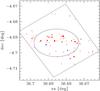 |
Fig. 5 Spatial distribution of red-sequence galaxies (red points), with symbols encoding brightness (brighter galaxies are indicated by larger points) and membership (spectroscopic members are indicated by filled points). The four blue spectroscopic members are also shown as blue points. The ellipse indicates the outermost detected X-ray isophote, and the slanted rectangle encloses the full-depth WFC3 field of view. |
4.3. Nature of the color–density relation at high redshift
In this section we show that the quenched galaxies in JKCS 041 are located preferentially at the center of the cluster potential, as is the case in low-redshift clusters. Figure 5 shows the spatial distribution of the red-sequence member galaxies (red points) compared with the extent of the X-ray emission (ellipse). Red-sequence galaxies (and the marginally blue galaxy ID447) are clearly concentrated within the zone of detected X-ray emission. The three blue members, in contrast, are located away from the cluster center. Clearly, the physical mechanism that quenched star formation in JKCS 041 left only a handful of star-forming galaxies that avoid the center as in nearby clusters (e.g., see Fig. 5 in Butcher & Oemler 1984 and; for the Coma cluster, Fig. 4 in Andreon 1996).
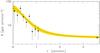 |
Fig. 6 Radial profile of red-sequence galaxies. The solid line is the mean fit and the shading indicates the 68% uncertainty. The control field data point has been arbitrary put at r = 3.6 for clarity. |
Figure 6 shows the circularized radial (= ) distribution of the red-sequence galaxies. Galaxies were counted within elliptical annuli and fitted with a beta model (Cavaliere & Fusco-Femiano 1976), accounting for Poisson fluctuations and for background contamination estimated using the GOODS-S control field. We also accounted for the boundary of the WFC3 field of view and took uniform priors on the model parameters. The shaded region in Fig. 6 shows the 68% error (highest posterior density interval). As in Sect. 4.2, the binned data are shown only for display purposes.
We found a core radius rc = 0.66 ± 0.18 arcmin (330 kpc), a radial slope β = 1.6 ± 0.6, and a central density value of 48 ± 13 galaxies arcmin-2. This is similar to the core radius rc = 0.62 ± 0.13 arcmin derived from the X-ray observations (Andreon et al. 2009), which was derived with β fixed at 2/3. The core radius of JKCS 041 resembles that in present-day clusters, which typically have rc ≈ 250 kpc (e.g., Bahcall 1975). The absence of star-forming galaxies in the core agrees with Raichoor & Andreon (2012a,b) who showed, based on a statistical analysis (i.e., without knowledge of individual galaxy membership), that the present-day star formation-density relation is already in place in JKCS 041 and that the processes responsible for the cessation of star formation in clusters are effective already at high redshift3.
A key result is that in JKCS 041 there is no evidence for an inversion of the local color–density relation, as has been suggested in the densest regions at high-z (Elbaz et al. 2007) and in a candidate cluster at similar redshift (Tran et al. 2010; but see Quadri et al. 2012, who instead claimed an elevated fraction of quiescent objects in the center of the same cluster). Nor do we find that 40% of galaxies in the cluster core have an intense episode of star formation (Brodwin et al. 2013).
4.4. Age–mass relation
In this section we measure the mean age–mass relation and its scatter for the red-sequence cluster members. The data quality and the proximity to the last major episode of star formation allow us to constrain for the first time the distribution of ages at a fixed mass. In particular, we can test for distributions that would indicate multiple epochs of star formation, across galaxies.
In Paper I, we fit grism spectra covering the rest-frame wavelength range ~3000 to ~6000 Å, along with photometry from u to [4.5] filters, with BC03 τ models characterized by a star formation time onset t0, the e-folding time τ, and dust attenuation. The galaxy spectra and spectral energy distributions (SED) basically constrain some degenerate combination of t0 and τ. Furthermore, the average stellar age of a stellar population is in general younger than t0. Therefore, following Longhetti et al. (2005), in the present paper we refer to ages tw that are weighted by the SFH and thus represent the average luminosity-weighted age of the population:  (1)Equation (1) has the following analytic solution for exponentially declining τ models of the SFH:
  (2)Because t0 is significantly higher than τ for the red-sequence galaxies, tw typically differs from t0 by ≈10 ± 5%, with a maximal difference of 30%.
Figure 7 shows the probability distributions for the SFH-weighted age of the red-sequence galaxies with spectra (technical details can be found in Appendix A). As mentioned before, the latter is essentially a mass-complete sample at H< 22.5 mag (2.5 mag brighter than the limit considered in earlier sections, because of the requirement of a spectrum) and a statistically representative sample to a limit that is 0.8 mag fainter (i.e., 0.3 dex lower). Galaxies in Fig. 7 are ordered by mass, with more massive objects at the top. Inspection of the figure qualitatively suggests that lower-mass galaxies have a younger age, about 1.0 Gyr, whereas massive galaxies have a broader age range and are possibly older. A notable exception is galaxy ID355, which is significantly younger than other galaxies of similar mass; as already remarked in Paper I, the presence of manifestly stronger Balmer lines in the grism spectrum and a brighter rest-frame UV continuum indicate that the age difference is genuine.
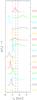 |
Fig. 7 Weighted age distribution of the spectroscopic members of JKCS 041that lie on the red sequence, sorted in order of decreasing mass (more massive toward the top). The three vertical lines correspond to zf = 2.5,3,3.5 Gyr from left to right. |
To investigate how the mean age depends on mass and to quantify the scatter in age at a given mass, we fit a linear relation between tw and mass. Our fitting procedure accounts for the error covariance between the mass and age measurements, for the presence of an intrinsic (possibly non-Gaussian) scatter at a given mass, and for the possible presence of outliers from the mean relation (such as ID355, for example; for details see Appendix A).
Figure 8 shows the data (colored clouds of dots), the mean fitted model (central solid line), its 68% error (solid, fan-shaped lines), and the intrinsic scatter (± 1σ, dotted lines). We verified that our fitting procedure correctly recovers the underlying parameters based on tests with simulated data, and we emphasize the importance of such tests in situations where the measurement errors are correlated and intrinsic scatter is significant.
The mean age of the red-sequence galaxies at M∗ = 1011 M⊙ is well determined: 1.1 ± 0.1 Gyr, i.e., 2.5 <zf< 2.7. Note that this small uncertainty includes the observational uncertainties (the finite number of galaxies and their scatter, errors on photometry and spectroscopy) but only a few model uncertainties: we marginalized over dust attenuation but assumed a fixed (solar) metallicity, a simple (exponential) shape for the SFH, and the validity of the BC03 model spectra.
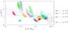 |
Fig. 8 Age–mass relation for red-sequence galaxies in JKCS 041. The clouds of colored points show the probability distribution for each individual galaxy, following the color coding in Fig. 7; ellipses show Laplace approximations. The straight solid line is the mean age–mass relation derived from these posteriors, based on the galaxy spectra and photometry. Fan-shaped lines delineate the error on the mean model (68% highest posterior interval), while the dotted lines indicate the intrinsic scatter (±1σ). |
The slope of the age–mass relation is 0.67 ± 0.35 Gyr per mass dex, consistent with that seen in Coma (e.g., Nelan et al. 2005). Because this slope is positive, it demonstrates that the mean stellar age depends on galaxy mass, with 95% probability. Red-sequence galaxies with log M/M⊙ ~ 11.5 are 1.4 Gyr old (i.e., zf = 2.9 if they were simple stellar populations, SSPs), while those with log M/M⊙ ~ 10.5 are 0.7 Gyr old (zf = 2.3). This age difference agrees with results found in Paper I (Sect. 5) by stacking the continuum-normalized spectra of the quiescent cluster members. Compared with the analysis of stacked spectra in Paper I, the present model allows for a more general SFH (an exponentially declining model, rather than a SSP) and a spread in ages at a given mass, but assumes a fixed solar metallicity. The analysis in Paper I showed that the spectral trends are too strong to be interpreted as arising from metallicity differences alone, justifying our current choice. We note that the mean age measured here agrees with that inferred from the location of the red sequence in the color−magnitude plane (Fig. 2), although this is not an independent test since the Y − H color is used in both age estimates.
There is a statistically significant intrinsic scatter σtw | M at a given mass, that is beyond that expected from the measurement errors. The inferred age scatter is 38 ± 9%, i.e., 370 ± 80 Myr at the median mass of our sample, log M/M⊙ ~ 11. Note that this small scatter cannot be due simply to a bias in our spectroscopic sample because of the high completeness discussed in Sect. 2. This age scatter is larger than the 160 ± 30 Myr previously estimated by Andreon (2011) at the 2.5 (combined) sigma level. This is mostly due to the high photometric redshift zphot = 2.2 assumed in that work, which implied that the red-sequence color z′ − J probes a bluer rest-frame band than it does at the true redshift zgrism = 1.803. This is significant because bluer bands are more sensitive to age differences.
In JKCS 041 we can probe closer to the epoch of star formation than in earlier studies of lower-redshift clusters, and yet we find a rather synchronous SFH, with a spread in ages of only 370 Myr. In particular, the precise spectroscopic ages (typical errors of 120 Myr, i.e., one-third of the age spread) allow us to resolve the distribution of ages and to verify whether there were multiple epochs of activity across galaxies. To test for this, we first computed standardized residuals around the fitted model: 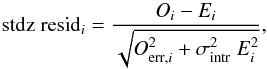 (3)where Oi and Ei are the observed and expected value of the ith galaxy and Oerr,i and σintr are the age error and the intrinsic scatter around the mean relation. We then quantified possible deviations using a quantile-quantile plot, using the Weibull (1939) estimate of the quantile. This approach has the advantage that it does not bin the data and is a powerful tool to check for non-Gaussian distributions of an unknown nature (as opposed to looking for a specific type of non-Gaussianity, such as asymmetry). Similar to the Kolmogorov-Smirnov test, this test basically compares the quantile of the observed values with those of a Gaussian distribution. We repeated this procedure for 5000 simulated samples each composed of 14 galaxies drawn from the model fitted on the real data, and with uncertainties and covariance as real data. 75% of random samples drawn from the null (Gaussian) model show larger discrepancies than those seen in the data. (This Bayesian p-value is computed by Markov Chain Monte Carlo, which allows us to account for the uncertainty in the relation scatter, intercept, and slope, see Andreon 2012a,b for details). This indicates that the age distribution (across galaxies) at fixed mass is indeed consistent with a Gaussian distribution, lending observational support to the widespread assumption that red-sequence cluster members follow a synchronous SFH.
4.5. Galaxy size–mass relation
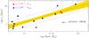 |
Fig. 9 Size–mass relation for JKCS 041. Lines show the mean fitted model and its uncertainty (solid line and yellow band), along with the intrinsic scatter (dotted line). Points are color-coded according to their location in the age–mass plane (Fig. 7): older (red) or younger (blue) than the mean relation by at least 1σintr, with black points indicating galaxies within ± 1σintr the mean age–mass relation. |
The evolution of the size–mass relation has been a topic of great interest over the past several years (see Paper I and references therein). Here we investigate whether the sizes of the red-sequence members of JKCS 041 at a given mass depend on their age. Such a scenario might be expected if the size–mass relation evolves because of the progressive quenching of larger galaxies over time.
Figure 9 shows the size–mass relation for the red-sequence galaxies in JKCS 041. We have excluded ID387, which has a bulge plus disk morphology and is not quiescent according to the UVJ criterion used in Paper I (in other words, its red color is attributed to dust rather than age). Circularized effective radii were derived in Paper I by fitting the WFC3 H-band surface brightness profiles with a Sersic model. The stellar mass was likewise derived in Paper I from spectra and photometry. For several galaxies the derived radii are smaller than the HST resolution and the WFC3 sampling; for these very compact systems, the assumption of a Sersic profile within the effective radius may be particularly important.
We fit the size–mass relation of JKCS 041 using a linear model with intrinsic scatter, deriving  (4)(solid line in Fig. 9) and an intrinsic scatter of 0.27 ± 0.06 dex in log re at fixed mass. Here we adopted a uniform prior for all parameters except the slope, for which we took instead a uniform prior on the angle. Assuming a Student-t distribution with 10 degrees of freedom for the scatter, which is more robust to the presence of outliers, does not change the results significantly.
While the sample of 14 galaxies is small, it is still five times larger than other samples of massive (log M/M⊙ ≳ 11) cluster galaxies at similar redshift for which a size has been measured: IDCS J1426.5+3508 has only two such quiescent galaxies, for example, and CL J1449+0856 has only one4.
To test whether the location of a galaxy in the size–mass plane depends on its stellar age, points in Fig. 8 have been color-coded according to their location in the age–mass plane. Red and blue symbols show galaxies that are older or younger than the mean age–mass relation by at least 1σintr, respectively, while those within ± 1σintr are black. Note that by comparing ages to the mean age–mass relation we naturally account for the correlation in these parameters. There is no evidence that older or younger galaxies have systematically larger or smaller sizes than the mean at a given mass. We note that this result is not sensitive to our particular choice of age bins.
5. Evolutionary trends
In the previous section we carried out a first comparison between JKCS 041 and low-redshift clusters. We found that quenching is fully in place over 2 orders of magnitude in stellar mass. We also found that the spatial distribution of red galaxies is similar to that of nearby clusters and is well described by a β profile of normal core radius. We found no reversal of the color-density (or cluster-centric distance) relation nor an unusual abundance of star-forming galaxies in the cluster core, in line with clusters in the local Universe. Having used the unique dataset for JKCS 041 to carry out unprecedented measurements of the galaxy cluster population at z = 1.80 we now construct comparison samples at lower and similar redshift to further investigate evolutionary trends and cluster-to-cluster variation.
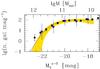 |
Fig. 10 Comparison of the luminosity function of red-sequence galaxies for JKCS 041 (blue points with large error bars, shading and lines as in previous figure) and Coma (black points; from Andreon 2008). The JKCS 041 LF has been re-normalized to the Coma cluster φ∗ for display purposes only. Labels on the upper x-axis indicate the stellar mass, derived from the H-band magnitude assuming our standard BC03 SSP settings with zf = 3. |
5.1. Evolution of the mass function
We investigated evolutionary trends in the faint-end slope of the red-sequence luminosity function (LF) by combining the results for JKCS 041 with those from 41 clusters taken from the literature for which high-quality data are available. We used the faint-end slope of the luminosity function as a measure of the relative abundance of faint galaxies compared with their more luminous counterparts. This is a more general approach than using other estimators such as the relative ratio between bright and faint objects (e.g., De Lucia et al. 2007; Stott et al. 2008; see also Andreon 2008).
Figure 10 compares the LF of JKCS 041 with that of the Coma cluster5. It is remarkable that the two LFs have indistinguishable shapes even though the look-back time to JKCS 041 is more than 10 Gyr. Figure 11 shows the faint-end slope as a function of redshift for a sample of 42 clusters, JKCS 041 and 41 clusters taken from the literature. The sample was chosen to satisfy the following criteria: the available colors straddle the rest-frame 4000 Å break; common filters are used for cluster and control field observations; the data are sufficiently deep (i.e., deeper than −18.2 mag in V band, as discussed by Andreon 2008; Crawford et al. 2009 and De Propris et al. 2013). As detailed in Table 1, we used 18 slope measurements, relative to 28 clusters (two points are average of several clusters) in the range 0 <z< 1.3 (Andreon 2008), 17 measurements at intermediate redshift (0.2 <z< 0.55, De Propris et al. 2013, 12 additional clusters) and one at z ~ 0.5 cluster (Crawford et al. 2009), for a total of 37 measurements of 42 clusters (including JKCS 041). In Appendix B we list the determinations excluded because they failed to satisfy these criteria.
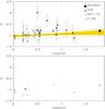 |
Fig. 11 Faint-end slope of the luminosity function of red-sequence galaxies of 42 clusters spanning over 10 Gyr of the age of the Universe. Top panel: open dots are from De Propris et al. (2013), the open square represents the Crawford et al. (2012) determination, while solid dots are our own work (this work or Andreon 2008 and references therein). Some points indicates stacks of two or ten clusters. The solid line is the mean model, while the shaded area represent the 68% uncertainty (highest posterior density interval) of the mean relation. Bottom panel: as in the top panel, with the amount of ink is proportional to the weight given to each point in the fit. |
We fit a linear relation to the data following Andreon & Hurn (2013): 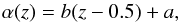 (5)with an intrinsic Gaussian scatter σintr. The parameter b is the evolution of the faint-end slope per unit redshift, while a is the mean faint-end slope at z = 0.5. We assumed uniform priors for the parameters within the physically acceptable ranges, except for the slope b, for which we adopted a uniform prior on the angle (which is the correct coordinate-independent form; see Andreon & Hurn 2010).
We find b = 0.08 ± 0.09, a = −0.98 ± 0.03, and σscatt = 0.17 ± 0.04 (see Fig. 11). The evolutionary term b is very small and consistent with zero. Our result is inconsistent with the evolution suggested by Rudnick et al. (2009) and Bildfell et al. (2012). The difference arises from the better quality of our data and the more rigorous selection applied in this study to the select the clusters, for which the background can be estimated using the same filters (see Appendix B).
We note that the faint-end slope of the LF has a sizable intrinsic cluster-to-cluster scatter σscatt = 0.17 ± 0.04. This needs to be taken into account when analyzing samples of clusters to avoid spurious results. Moreover, proper weight should be given in the fit to each cluster, since the uncertainties differ widely across the sample. A visual representation of the importance of each data point is given in the bottom panel of Fig. 11. The weight of each data point is proportional to that adopted in the fit, which takes into account errors on measurement, the intrinsic scatter, and the number of clusters per measurement. The more informative points are, in strict order of importance, the stack of 10 clusters at z = 0.25, the clusters at the extremes in redshift (JKCS 041, Coma and Abell 2199), and the stack of the two Lynx clusters (at z = 1.26). This plot qualitatively confirms the shallow, if any, (and statistically insignificant) evolution of the faint-end slope over Δz = 2.
We note that our conclusions about the lack of evolution of the faint red-sequence galaxies are robust with respect to the methodology. For example, by using the luminous-over-faint ratio as defined by De Lucia et al. (2007), we find L/F = 0.61 ± 0.17, consistent with measurements at lower redshift (Andreon 2008; Capozzi et al. 2010; Bildfell et al. 2012; Valentinuzzi et al. 2011). Naturally, several arguments (e.g., Andreon 2008) lead us to expect evolution for the red sequence, and absence of evidence should not be interpreted as evidence of absence. Interestingly, the quality of our data set allows us to set a stringent upper limit to the change of the faint-end slope b< 0.23 with 95% probability.
Another interesting topic is the evolution of the bright end of the red sequence. Most studies of clusters at z< 1.4, starting perhaps with Aragon-Salamanca et al. (1993), found it to be consistent with passive evolution (see also, e.g., Andreon et al. 2008; De Propris et al. 2013). Here we take advantage of the extreme redshift of JKCS 041 to revisit this measurement in combination with the high-quality data sample used for the faint-end slope.
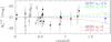 |
Fig. 12 Characteristic magnitude of red-sequence galaxies across 10 Gyr. Locii of constant |
Figure 12 shows the evolution of the characteristic magnitude  with redshift6. For illustration, a number of model predictions (lines indicating
  mag) are shown for different formation redshifts zf and for the 2007 version of the Bruzual & Charlot (2003) models. It is clear that data at z< 1.5 are insufficient to distinguish between models. At the redshift of JKCS 041, the differences between models are more significant. Models with zf = 5 underpredict the brightness of the galaxies in JKCS 041, while models with zf = 2.5−3 better match the data.
With this complete spectroscopic sample showing a fully populated red sequence at all masses, we do not confirm the high merger activity in high-redshift clusters, which was suggested based on the statistically estimated paucity of massive >L∗ members on the red sequence (e.g., Mancone et al. 2010).
To summarize, the bright end of the luminosity function of the red sequence evolves as a passively evolving stellar population formed at ~2.5 <zf ≲ 5. We note that this conclusion does not rely on assuming a constant faint-end slope and is robust with respect to systematic uncertainties in stellar population models. More clusters at z> 1.5 are required to improve this estimate.
5.2. Evolution of the galaxy size–mass relation
As a first approach to understanding evolution of the mass–size relation, we compared JKCS 041 with the Coma cluster, chosen because it has the richest and most controlled set of data: 75 early-type (S0 or earlier) galaxies more massive than log M/M⊙ = 10.7, comprising a mass-complete sample with high-resolution (~0.6 kpc) imaging data (Andreon et al. 1996, 1997). Stellar masses were derived from R magnitudes assuming the standard BC03 setting with zf = 3. Effective radiii were derived from fitting model growth curves7 from de Vaucouleurs (1977) to the measured galaxy growth curves (see Michard 1985 for fitting details).
The fit of the size–mass relation to Coma galaxies gives  (6)with an intrinsic scatter of 0.16 ± 0.01 dex in log re at a given mass (see also Fig. 13). This is consistent, within the errors, with the relation found for JKCS 041, as also illustrated by the locus of the 68 and 95% probability contours shown in Fig. 14.
The size–mass relation of red-sequence quiescent galaxies in JKCS 041 is consistent with the relation for early-type galaxies in clusters at z ~ 0 within the uncertainties arising from our sample of 14 systems, which represent a fivefold increase in the number of high-redshift galaxies compared with other structures at similar redshifts, and we place a 95% confidence upper limit of 0.4 dex on size growth at fixed stellar mass (at 1011 M⊙) between z = 1.8 and z = 0, or, equivalently, a 1σ upper limit of ~0.11 per unit redshift.
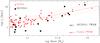 |
Fig. 13 Size–mass relation for JKCS 041 (black squares) and Coma (red points) galaxies. The figure also presents the mean fitted model (solid line) and the one-sigma intrinsic scatter (dotted line) around the relation for Coma galaxies. |
At face value, the best-fit JKCS 041 mass–size relation indicates a 0.22 (=0.33−0.11) dex change in the size of cluster galaxies relative to z = 0, in the sense that Coma galaxies are larger than those in JKCS 041. In the same redshift range, the mean change in the field from z = 1.8 to 0 is 0.47 dex (Newman et al. 2012), giving a first indication that size evolution might occur earlier in clusters. The suggested indication is also indirectly implied by the environmental dependence of the size evolution found in other works (e.g., Cooper et al. 2011; Lani et al. 2013; Bassett et al. 2013). However, this is one of the first works that presents a direct cluster-to-cluster comparison across redshifts. A confirmation of this indication would be extremely valuable.
This comparison clearly relies on the choice of the low-redshift comparison cluster, a few assumptions, and slightly different methods to derive mass and re. However, these do not introduce systematics, as justified in Appendix C. A more complete analysis of this issue necessitating a comparison with many clusters along the 0 <z< 1.8 redshift range will be addressed in a future paper.
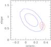 |
Fig. 14 68 and 95 % probability contours for JKCS 041 (blue) and Coma (red) size–mass relation. |
Cluster redshift, faint–end slope α and characteristic magnitude .
6. Discussion
6.1. Comparisons with other high redshift clusters
Although studies of a single cluster at z = 1.803 will not allow us to infer the evolutionary properties of the population of distant cluster galaxies as a whole, the high-quality data available for JKCS 041 allow us to perform unique analyses that are currently not possible for other clusters at comparable redshift.
To illustrate the advantages, we compare the red sequence in JKCS 041 with that in the z = 1.75 cluster IDCS J1426.5+3508 (Stanford et al. 2012). The latter data are complete to H ≲ 22.5 mag (set by the blue filter), which is unfortunately too bright for assessing the relative proportion of luminous and faint members. This is the general situation for most other distant clusters: a direct comparison of the faint end of the red sequence is not yet possible because of the lack of similarly deep data in two bands straddling the 4000 Å break.
Even studies of the luminous end of the cluster red sequence are often hampered by confusion regarding cluster membership. For example, IDCS J1426.5+3508 has only two spectroscopically confirmed members. Although the magnitude of the brightest member is H = 20.4 mag both in IDCS J1426.5+3508 and JKCS 041, the second-brightest red-sequence (candidate) galaxy in IDCS J1426.5+3508 is ≳0.8 mag fainter, while JKCS 041 has three galaxies within this range. Therefore, quantitative statements on the nature of the red sequence in IDCS J1426.5+3508 must await a substantial increase in spectroscopic redshift coverage. It is also possible to compare with the luminous end of the red sequence in the CL J1449+0856 structure at z = 1.99 (Gobat et al. 2009, 2013). However, there is only one galaxy of similar luminosity (with H ≲ 22.5 mag, “rescaled” to the JKCS 041 redshift and accounting for the different H filter used), which implies a significant difference with JKCS 041, where we have ~12 cluster galaxies.
The well-populated luminous red sequence in JKCS 041 indicates that the lack of bright red galaxies in candidate high-redshift clusters (e.g., Mancone et al. 2010, see Andreon 2013) is not a universal phenomenon. The paucity of star-forming galaxies with log M/M⊙> 10.5 argues against the Brodwin et al. (2013) hypothesis that z ≳ 1.4 represents a “firework era” for cluster galaxies (e.g., Hilton et al. 2010; Fassbender et al. 2011). Brodwin et al. (2013) claimed that 40% of log M/M⊙> 10.1 galaxies in many clusters are undergoing starbursts with ≳50 M⊙ yr-1) galaxies deep into the cluster center. This is clearly not the case in JKCS 041. However, the quality of the data of JKCS 041 is unique and unmatched by the Brodwin et al. (2013) data set: quenched galaxies at the studied redshifts might be under-represented as a result of the insufficient depth of the data8. Consequently, the starburst component may be overestimated. Furthermore, at r ~ 1.5 Mpc, the radial profile of the SFR per unit area seems to flatten at 85 ± 5 M⊙ yr-1 arcmin-2, indicating either that the clusters are more extended than this or that the background contribution is underestimated. However, only three starforming members have been confirmed in each of the two most distant clusters in Brodwin et al. (2013) using grism spectroscopy to a depth an order of magnitude more sensitive in star formation (Zeimann et al. 2013). On the other end, if the results by Brodwin et al. (2013) will be confirmed, this would indicate a cluster-to-cluster variance in the effectiveness of the environmental-dependent quenching.
6.2. The significance of the JKCS 041 cluster
The properties of JKCS 041 are remarkable in many ways. The cluster mass will likely grow by a factor of about 3 by z = 0 (Fakhouri et al. 2010) to emerge locally as a system similar to the Coma cluster. Yet, even at z = 1.803, JKCS 041 already resembles many nearby clusters: it has a similar core radius, a tight red sequence with no deficit of faint or bright red galaxies, few star-forming galaxies in its central region (about 0.7r500). Moreover, its age–mass and size–mass relations agree with those derived in nearby clusters, given the uncertainties set by the JKCS 041 sample size. JKCS 041 contrasts with its adjacent z = 1.8 field as Coma does with the local field: from a comparison with field galaxies of the same mass at z ~ 1.8, in Paper I we found that environmental quenching (i.e., the cluster environment) is responsible for more than half the quenched galaxies, quite similar to what is observed at z ~ 0.3−0.45 and z ~ 0 (Andreon et al. 2006). At z = 1.8, the comparison between quiescent galaxies in the field and JKCS 041 shows that the cluster environment affects the proportion of quenched galaxies, but not when they were quenched (Paper I), an inference similar to what is found locally. In short, the environment determines the space density of each type but not the internal properties of the type, which are the same across all environments (Andreon 1996). These results are surprising when one considers that the last major episode of star formation was at most 2 Gyr, and more typically 1 Gyr, earlier. In this remarkably short time JKCS 041 has already achieved a resemblance to nearby clusters, a similarity it presumably must maintain during its sizable continued mass growth over the next 10 Gyr.
We suggest the following scenario to explain the observations: first, cluster growth involves acquiring additional material with a composition that already resembles that of the main progenitor and not distributing it randomly in the cluster. Both are well-known features of the hierarchical paradigm of galaxy formation. Galaxies in a cluster at a given time arise from regions of above-average density at all epochs of their history (e.g., Kaiser 1984). At low (e.g., Balogh et al. 1999) and intermediate redshift (Andreon et al. 2005) and in JKCS 041 (Raichoor & Andreon 2012a), there is a high fraction of quenched galaxies well past the virial radius. At low redshift at least, the high-mass end of the mass function of galaxies of a given morphology are environment-independent (e.g., Bingelli et al. 1988; Andreon 1998; Pahre et al. 1998). Collecting material in a self-similar way helps to maintain a fixed faint-slope of the mass function and a fixed characteristic mass, while the luminosity function normalization φ∗ and the cluster richness and mass are free to increase.
The radial dependencies (e.g., the core radius, the lack of star-forming galaxies in the cluster core) are maintained since, in a hierarchical picture, the cluster-centric distance distribution of infalling galaxies is not uniform. Smith et al. (2012) illustrated this convincingly in the case of the environmental quenching: galaxies in the cluster core fell inwards at an earlier times, on average. This preferentially builds up the peripheral regions, outside the field of view considered here.
After submitting this paper we became aware of Cen (2014), who presented state-of-art galaxy formation simulations of a region centered on a galaxy cluster. These simulations reproduce our findings: there is no lack of faint red galaxies, quenching is found to be more efficient, but not faster in dense environments, faint red galaxies are younger than their massive cousins, mass growth occurs mostly in the blue cloud and therefore the characteristic mass of red sequence galaxies should not strongly evolve with redshift, correlation between observables of red galaxies, because the age–mass or mass–size relations are largely inherited and therefore mantained with z.
7. Summary
The unique depth of two-color near-infrared HST images (complete above an effective stellar mass log M/M⊙ = 9.8) and spectroscopy (complete to log M/M⊙ = 10.8 independently of the spectral type) of the z = 1.803 JKCS 041 cluster has allowed us to investigate in detail the cluster mass, the spatial distribution of red galaxies, the mass/luminosity function, the color−magnitude diagram, and the age–mass and size–mass relations.
The abundance of high-quality data in JKCS 041 is apparent by comparing the color–magnitude diagram with those of other high-redshift clusters. For the first time, it was possible to eliminate foreground galaxies to H< 22.5 mag via spectroscopy. Statistically, it is possible to account for contamination to H = 25 mag. This provides the first cluster red sequence at this redshift over two orders of magnitude in stellar mass. Furthermore, the detailed spectroscopy (and 12-band photometry) enables us to estimate the stellar ages for a complete sample.
Our analyses provided the following results:
-
1.
The JKCS 041 cluster mass, determined from four different methods (X-ray temperature, X-ray luminosity, gas mass, and cluster richness), is consistently log M200/M⊙ ≳ 14.2, demonstrating unequivocally that JKCS 041 is a massive system that will most likely become a present-day cluster similar to the Coma cluster.
-
2.
The JKCS 041 red sequence of quiescent members is remarkably well-formed: all massive cluster members are red, and there is no deficit of faint red galaxies down to a stellar mass of log M/M⊙ = 9.8. Consequently, quenching has already occurred over two orders of magnitude in mass. By comparison with field galaxies at a similar redshift (Paper I), environmental quenching must be responsible for more than half the red galaxies.
-
3.
The red-sequence galaxies in JKCS 041 are concentrated towards the cluster center with a spatial distribution well described by a beta profile with core radius 330 kpc. Blue galaxies represent a minority and avoid the cluster center, as in nearby clusters.
-
4.
The JKCS 041 red sequence is interpreted as being mostly an age sequence with less massive galaxies significantly younger. The age scatter at a given mass is 38 ± 9%, that is, 370 Myr at log M/M⊙ = 11. The star-formation-history weighted age is typically 1.1 ± 0.1 Gyr, corresponding to a formation epoch zf = 2.6 ± 0.1.
-
5.
The size–mass relation of red-sequence quiescent galaxies in JKCS 041 is consistent with that observed locally given the uncertainties arising from the smaller sample size at high redshift. Given that the mean change in the field from z = 1.8 to 0 is larger (0.47 dex vs. 0.22 dex, at face value), this is a first indication that size evolution might occur earlier in clusters.
-
6.
Complementing JKCS 041 data with data from 41 clusters at lower redshift, the shape of the galaxy mass function of red-sequence galaxies is unaltered over the past 10 Gyr. We derived stringent upper limits on any change of the faint-end slope and characteristic mass of the distribution.
Despite the proximity in time to the quenching era and the likely three-fold increase in mass over the subsequent 10 Gyr, JKCS 041 is already remarkably similar to present-day clusters. We provided a qualitative scenario where this occurs within the context of the hierarchical paradigm of galaxy formation.
This region (i.e., the factor 1.2 ×) was chosen as a compromise between maximizing the number of enclosed red-sequence cluster members and minimizing the number of random interlopers, as judged from the control field.
Stellar ages derived from the grism spectra are discussed in Sect. 4.4.
As mentioned in these papers, the analysis assumed zphot = 1.8 for consistency with galaxy colors, and thus requires no revision, even though the JKCS 041 points are plotted at zphot = 2.2 for consistency with earlier estimates of the cluster redshift.
We accounted for differences in mass definitions across works.
The H-band luminosity at z = 1.803 has been converted to the present-day V-band luminosity assuming our standard BC03 setting with zf = 3 to account for 10 Gyr of luminosity evolution. Note that we would have obtained an indistinguishable result by using the revised version of the Bruzual & Charlot (2003) model with a Chabrier IMF (apart from the obvious common shift in mass of both Coma and JKCS 041 galaxies).
 is obtained from the absolute characteristic magnitude in the band of observation (close to the V-band rest-frame) evolved to z = 0 and converted into the V band by adopting a BC03 SSP model with zf = 3.
Note that these are the mean observed growth curves of galaxies of different morphological types, not r1/4 growth curves.
Acknowledgments
S.A. acknowledges Veronica Strazzullo for comments on an early version of this draft and Stefano Ettori and Fabio Gastaldello for the JKCS 041 gas mass computation. We acknowledge HST, program 12927, and CFHT, see full-text acknowledgements at http:// [0]www. [0]stsci. [0]edu/ [0]hst/ [0]proposing/ [0]documents/ [0]cp/ [0]10_ [0]Proposal_ [0]Implementation12. [0]html and http:// [0]www. [0]cfht. [0]hawaii. [0]edu/ [0]Science/ [0]CFHLS/ [0]cfhtlspublitext. [0]html. A.R. acknowledges financial contribution from the agreement ASI-INAF I/009/10/0 and from Osservatorio Astronomico di Brera.
References
- Aguerri, J. A. L., Iglesias-Paramo, J., Vilchez, J. M., & Muñoz-Tuñón, C. 2004, AJ, 127, 1344 [NASA ADS] [CrossRef] [Google Scholar]
- Andreon, S. 1996, A&A, 314, 763 [NASA ADS] [Google Scholar]
- Andreon, S. 1998, A&A, 336, 98 [NASA ADS] [Google Scholar]
- Andreon, S. 2006, MNRAS, 369, 969 (A06) [NASA ADS] [CrossRef] [Google Scholar]
- Andreon, S. 2008, MNRAS, 386, 1045 (A08) [NASA ADS] [CrossRef] [Google Scholar]
- Andreon, S. 2010, MNRAS, 407, 263 [NASA ADS] [CrossRef] [Google Scholar]
- Andreon, S. 2011, A&A, 529, L5 [NASA ADS] [CrossRef] [EDP Sciences] [Google Scholar]
- Andreon, S. 2012a, A&A, 548, A83 [NASA ADS] [CrossRef] [EDP Sciences] [Google Scholar]
- Andreon, S. 2012b, in Astrostatistical Challenges for the New Astronomy, ed. J. Hilbe (Springer Series on Astrostatistics) [Google Scholar]
- Andreon, S. 2013, A&A, 554, A79 [NASA ADS] [CrossRef] [EDP Sciences] [Google Scholar]
- Andreon, S., & Hurn, M. A. 2010, MNRAS, 404, 1922 [NASA ADS] [Google Scholar]
- Andreon, S., & Huertas-Company, M. 2011, A&A, 526, A11 [NASA ADS] [CrossRef] [EDP Sciences] [Google Scholar]
- Andreon, S., & Hurn, M. A. 2013, Stat. Anal. Data min., 6, 15 [Google Scholar]
- Andreon, S., Davoust, E., Michard, R., Nieto, J.-L., & Poulain, P. 1996, A&AS, 116, 429 [NASA ADS] [CrossRef] [EDP Sciences] [Google Scholar]
- Andreon, S., Davoust, E., & Poulain, P. 1997, A&AS, 126, 67 [NASA ADS] [CrossRef] [EDP Sciences] [Google Scholar]
- Andreon, S., Pelló, R., Davoust, E., Domínguez, R., & Poulain, P. 2000, A&AS, 141, 113 [NASA ADS] [CrossRef] [EDP Sciences] [Google Scholar]
- Andreon, S., Punzi, G., & Grado, A. 2005, MNRAS, 360, 727 [NASA ADS] [CrossRef] [Google Scholar]
- Andreon, S., Quintana, H., Tajer, M., Galaz, G., & Surdej, J. 2006, MNRAS, 365, 915 [NASA ADS] [CrossRef] [Google Scholar]
- Andreon, S., Puddu, E., De Propris, R., & Cuillandre, J.-C. 2008, MNRAS, 385, 979 (A+08) [NASA ADS] [CrossRef] [Google Scholar]
- Andreon, S., Maughan, B., Trinchieri, G., & Kurk, J. 2009, A&A, 507, 147 [NASA ADS] [CrossRef] [EDP Sciences] [Google Scholar]
- Aragon-Salamanca, A., Ellis, R. S., Couch, W. J., & Carter, D. 1993, MNRAS, 262, 764 [NASA ADS] [CrossRef] [Google Scholar]
- Bahcall, N. A. 1975, ApJ, 198, 249 [NASA ADS] [CrossRef] [Google Scholar]
- Bassett, R., Papovich, C., Lotz, J. M., et al. 2013, ApJ, 770, 58 [NASA ADS] [CrossRef] [Google Scholar]
- Bertin, E., & Arnouts, S. 1996, A&AS, 117, 393 [NASA ADS] [CrossRef] [EDP Sciences] [Google Scholar]
- Bielby, R., Hudelot, P., McCracken, H. J., et al. 2012, A&A, 545, A23 [NASA ADS] [CrossRef] [EDP Sciences] [Google Scholar]
- Bildfell, C., Hoekstra, H., Babul, A., et al. 2012, MNRAS, 425, 204 [NASA ADS] [CrossRef] [Google Scholar]
- Bower, R. G., Lucey, J. R., & Ellis, R. S. 1992, MNRAS, 254, 601 [NASA ADS] [CrossRef] [Google Scholar]
- Brodwin, M., Stanford, S. A., Gonzalez, A. H., et al. 2013, ApJ, 779, 138 [NASA ADS] [CrossRef] [Google Scholar]
- Bruzual, G., & Charlot, S. 2003, MNRAS, 344, 1000 [NASA ADS] [CrossRef] [Google Scholar]
- Capozzi, D., Collins, C. A., & Stott, J. P. 2010, MNRAS, 403, 1274 [NASA ADS] [CrossRef] [Google Scholar]
- Cavaliere, A., & Fusco-Femiano, R. 1976, A&A, 49, 137 [NASA ADS] [Google Scholar]
- Cen, R. 2014, ApJ, 781, 38 [NASA ADS] [CrossRef] [Google Scholar]
- Cooper, M. C., Aird, J. A., Coil, A. L., et al. 2011, ApJS, 193, 14 [Google Scholar]
- Crawford, S. M., Bershady, M. A., & Hoessel, J. G. 2009, ApJ, 690, 1158 (C+09) [NASA ADS] [CrossRef] [Google Scholar]
- De Lucia, G., Poggianti, B. M., Aragón-Salamanca, A., et al. 2007, MNRAS, 374, 809 [NASA ADS] [CrossRef] [Google Scholar]
- De Propris, R., Stanford, S. A., Eisenhardt, P. R., Dickinson, M., & Elston, R. 1999, AJ, 118, 719 [NASA ADS] [CrossRef] [Google Scholar]
- De Propris, R., Phillipps, S., & Bremer, M. 2013, MNRAS, 434, 3469 (DeP+13) [NASA ADS] [CrossRef] [Google Scholar]
- de Vaucouleurs, G. 1948, Ann. Astrophys., 11, 247 [Google Scholar]
- de Vaucouleurs, G. 1977, ApJ, 33, 211 [Google Scholar]
- Dressler, A. 1980, ApJ, 236, 351 [NASA ADS] [CrossRef] [Google Scholar]
- Elbaz, D., Daddi, E., Le Borgne, D., et al. 2007, A&A, 468, 33 [NASA ADS] [CrossRef] [EDP Sciences] [Google Scholar]
- Ettori, S., Tozzi, P., Borgani, S., & Rosati, P. 2004, A&A, 417, 13 [NASA ADS] [CrossRef] [EDP Sciences] [Google Scholar]
- Fakhouri, O., Ma, C.-P., & Boylan-Kolchin, M. 2010, MNRAS, 406, 2267 [NASA ADS] [CrossRef] [Google Scholar]
- Fassbender, R., Nastasi, A., Böhringer, H., et al. 2011, A&A, 527, L10 [NASA ADS] [CrossRef] [EDP Sciences] [Google Scholar]
- Galametz, A., Stern, D., Pentericci, L., et al. 2013, A&A, 559, A2 [NASA ADS] [CrossRef] [EDP Sciences] [Google Scholar]
- Gobat, R., Daddi, E., Onodera, M., et al. 2011, A&A, 526, A133 [NASA ADS] [CrossRef] [EDP Sciences] [Google Scholar]
- Gobat, R., Strazzullo, V., Daddi, E., et al. 2013, ApJ, 776, 9 [NASA ADS] [CrossRef] [Google Scholar]
- Grogin, N. A., Kocevski, D. D., Faber, S. M., et al. 2011, ApJS, 197, 35 [NASA ADS] [CrossRef] [Google Scholar]
- Guo, Y., Ferguson, H. C., Giavalisco, M., et al. 2013, ApJS, 207, 24 [NASA ADS] [CrossRef] [Google Scholar]
- Jannuzi, B. T., & Dey, A. 1999, Photometric Redshifts and the Detection of High Redshift Galaxies, eds. R. Weymann, L. Storrie-Lombardi, M. Sawicki, & R. Brunner, ASP Conf. Ser., 191, 111 [Google Scholar]
- Hilton, M., Lloyd-Davies, E., Stanford, S. A., et al. 2010, ApJ, 718, 133 [NASA ADS] [CrossRef] [Google Scholar]
- Hoyos, C., den Brok, M., Verdoes Kleijn, G., et al. 2011, MNRAS, 411, 2439 [NASA ADS] [CrossRef] [Google Scholar]
- Houghton, R. C. W., Davies, R. L., Dalla Bontà, E., & Masters, R. 2012, MNRAS, 423, 256 [NASA ADS] [CrossRef] [Google Scholar]
- Kodama, T., & Arimoto, N. 1997, A&A, 320, 41 [NASA ADS] [Google Scholar]
- Koekemoer, A. M., Faber, S. M., Ferguson, H. C., et al. 2011, ApJS, 197, 36 [NASA ADS] [CrossRef] [Google Scholar]
- Lani, C., Almaini, O., Hartley, W. G., et al. 2013, MNRAS, 435, 207 [NASA ADS] [CrossRef] [Google Scholar]
- Le Fèvre, O., Vettolani, G., Garilli, B., et al. 2005, A&A, 439, 845 [NASA ADS] [CrossRef] [EDP Sciences] [Google Scholar]
- Le Fevre, O., Cassata, P., Cucciati, O., et al. 2013, A&A, 559, A14 [NASA ADS] [CrossRef] [EDP Sciences] [Google Scholar]
- Lemaux, B. C., Gal, R. R., Lubin, L. M., et al. 2012, ApJ, 745, 106 [NASA ADS] [CrossRef] [Google Scholar]
- Lidman, C., Rosati, P., Tanaka, M., et al. 2008, A&A, 489, 981 [NASA ADS] [CrossRef] [EDP Sciences] [Google Scholar]
- Longhetti, M., Saracco, P., Severgnini, P., et al. 2005, MNRAS, 361, 897 [NASA ADS] [CrossRef] [Google Scholar]
- Johnston, D. E., Sheldon, E. S., Wechsler, R. H., et al. 2007, unpublished [arXiv:0709.1159] [Google Scholar]
- Mancone, C. L., Gonzalez, A. H., Brodwin, M., et al. 2010, ApJ, 720, 284 [NASA ADS] [CrossRef] [Google Scholar]
- Mancone, C. L., Baker, T., Gonzalez, A. H., et al. 2012, ApJ, 761, 141 [NASA ADS] [CrossRef] [Google Scholar]
- Menci, N., Rosati, P., Gobat, R., et al. 2008, ApJ, 685, 863 [NASA ADS] [CrossRef] [Google Scholar]
- Michard, R. 1985, A&AS, 59, 205 [NASA ADS] [Google Scholar]
- Moster, B. P., Somerville, R. S., Newman, J. A., & Rix, H.-W. 2011, ApJ, 731, 113 [Google Scholar]
- Navarro, J. F., Frenk, C. S., & White, S. D. M. 1997, ApJ, 490, 493 [NASA ADS] [CrossRef] [Google Scholar]
- Nelan, J. E., Smith, R. J., Hudson, M. J., et al. 2005, ApJ, 632, 137 [NASA ADS] [CrossRef] [Google Scholar]
- Newman, A. B., Ellis, R. S., Bundy, K., & Treu, T. 2012, ApJ, 746, 162 [NASA ADS] [CrossRef] [Google Scholar]
- Newman, A. B., Ellis, R. S., Andreon, S., et al. 2013, ApJ, submitted [arXiv:1310.6754] [Google Scholar]
- Oemler, A., Jr. 1974, ApJ, 194, 1 [NASA ADS] [CrossRef] [Google Scholar]
- Pahre, M. A. 1999, ApJS, 124, 127 [NASA ADS] [CrossRef] [Google Scholar]
- Pahre, M. A., Djorgovski, S. G., & de Carvalho, R. R. 1998, AJ, 116, 1591 [NASA ADS] [CrossRef] [Google Scholar]
- Paolillo, M., Andreon, S., Longo, G., et al. 2001, A&A, 367, 59 [Google Scholar]
- Plummer M. 2008, JAGS Version 1.0.3 user manual, http:// [0]calvin. [0]iarc. [0]fr/ [0]~martyn/ [0]software/ [0]jags/ [0]jags_ [0]user_ [0]manual. [0]pdf [Google Scholar]
- Quadri, R. F., Williams, R. J., Franx, M., & Hildebrandt, H. 2012, ApJ, 744, 88 [NASA ADS] [CrossRef] [Google Scholar]
- Raichoor, A., & Andreon, S. 2012a, A&A, 543, A19 [NASA ADS] [CrossRef] [EDP Sciences] [Google Scholar]
- Raichoor, A., & Andreon, S. 2012b, A&A, 537, A88 [NASA ADS] [CrossRef] [EDP Sciences] [Google Scholar]
- Rudnick, G., von der Linden, A., Pelló, R., et al. 2009, ApJ, 700, 1559 [NASA ADS] [CrossRef] [Google Scholar]
- Sandage, A., Tammann, G. A., & Yahil, A. 1979, ApJ, 232, 352 [NASA ADS] [CrossRef] [EDP Sciences] [Google Scholar]
- Santos, J. S., Altieri, B., Popesso, P., et al. 2013, MNRAS, 433, 1287 [NASA ADS] [CrossRef] [Google Scholar]
- Sersic, J. L. 1968, Atlas de galaxias australes (Cordoba, Argentina: Observatorio Astronomico) [Google Scholar]
- Schechter, P. 1976, ApJ, 203, 297 [Google Scholar]
- Shen, S., Mo, H. J., White, S. D. M., et al. 2003, MNRAS, 343, 978 [NASA ADS] [CrossRef] [Google Scholar]
- Stanford, S. A., Eisenhardt, P. R., & Dickinson, M. 1998, ApJ, 492, 461 [NASA ADS] [CrossRef] [Google Scholar]
- Stanford, S. A., Brodwin, M., Gonzalez, A. H., et al. 2012, ApJ, 753, 164 [NASA ADS] [CrossRef] [Google Scholar]
- Stott, J. P., Pimbblet, K. A., Edge, A. C., Smith, G. P., & Wardlow, J. L. 2009, MNRAS, 394, 2098 [NASA ADS] [CrossRef] [Google Scholar]
- Strazzullo, V., Rosati, P., Pannella, M., et al. 2010, A&A, 524, A17 [NASA ADS] [CrossRef] [EDP Sciences] [Google Scholar]
- Strazzullo, V., Gobat, R., Daddi, E., et al. 2013, ApJ, 772, 118 [NASA ADS] [CrossRef] [Google Scholar]
- Tozzi, P., Santos, J. S., Nonino, M., et al. 2013, A&A, 551, A45 [NASA ADS] [CrossRef] [EDP Sciences] [Google Scholar]
- Tran, K.-V. H., Papovich, C., Saintonge, A., et al. 2010, ApJ, 719, L126 [CrossRef] [Google Scholar]
- Treu, T., Ellis, R. S., Kneib, J.-P., et al. 2003, ApJ, 591, 53 [NASA ADS] [CrossRef] [Google Scholar]
- Valentinuzzi, T., Fritz, J., Poggianti, B. M., et al. 2010, ApJ, 712, 226 [NASA ADS] [CrossRef] [Google Scholar]
- Valentinuzzi, T., Poggianti, B. M., Fasano, G., et al. 2011, A&A, 536, A34 [NASA ADS] [CrossRef] [EDP Sciences] [Google Scholar]
- Weibull, W. 1939, The Statistical Theory of the Strength of Materials, IVA Handlingar, Royal Swedish Academy of Engineering Sciences, No. 151 (Generalstabens litografiska anstalts forlag) [Google Scholar]
- Williams, R. J., Quadri, R. F., Franx, M., van Dokkum, P., & Labbé, I. 2009, ApJ, 691, 1879 [NASA ADS] [CrossRef] [Google Scholar]
- Zeimann, G., Stanford, S. A., Brodwin, M., et al. 2013, ApJ, 779, 137 [NASA ADS] [CrossRef] [Google Scholar]
- Zwicky, F. 1957, Morphological astronomy (Berlin: Springer) [Google Scholar]
Appendix A: details of fitting the age–mass relation
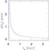 |
Fig. A.1 Implicit prior on the SFH-weighted age tw used in Paper I when fitting galaxy spectra and photometry, arising from the log-uniform priors on t0 and τ. In the present paper we prefer a uniform prior on tw and so have divided out this prior. |
Based on the posterior probability distributions for t0 and τ obtained in Paper I (Sect. 4) by fitting the grism spectra and 12-band photometry, we computed the posterior probability distribution of the SFH-weighted age tw using Eq. (2). The posteriors derived in this way assume a prior on tw, shown in Fig. A.1, that arises from the bounded log-uniform priors used for t0 and τ. To base our results for tw on a uniform prior in that parameter, we divided the posterior distributions by the prior in Fig. A.1. The resulting distributions are shown in Figs. 7 and 8.
The age–mass posterior probability distribution, p(tw,M), can be approximated by a multi-normal distribution with parameters given by the moments of p(tw,M), which are outlined in Fig. 8 as ellipses. Note that this approach naturally accounts for the known covariance between the measured mass and age. The multi-normal approximation is sufficiently accurate for our purposes, since the scatter in age at a given mass is dominated by intrinsic galaxy-to-galaxy variation.
We fit the relation between mass and SFH-weighted age tw with a model that is linear in the logarithm of the stellar mass and allows for intrinsic scatter, which is clearly visible when inspecting Figs. 7 and 8. Given that ages can only be positive, we modeled a scatter in log tw (scatter in linear units would allow for unphysical negative ages). To deal with potential outliers, such as ID 355 (whose young age for its mass was discussed in Sect. 4.4), we adopted an outlier-resistant model of the intrinsic scatter: a Student-t distribution of log tw with 10 degrees of freedom, which has more extended tails than a normal distribution. We took a uniform prior on the parameters, except for the slope, for which we instead used a uniform distribution in the arctan of the slope (see Andreon & Hurn 2010 for details). Finally, we computed the posterior probability distribution using JAGS (Plummer 2008), a standard MCMC sampler.
Appendix B: Literature measurements of the faint-end slope of the red-sequence luminosity function
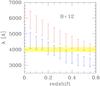 |
Fig. B.1 Rest-frame λ sampling of the adopted filters for the clusters studied in Bildfell et al. (2012) (z< 0.57). The shaded (yellow) band marks the 4000 Å break. |
An accurate measurement of the red-sequence LF requires that the filters used tightly sample the 4000 Å break, that the same filters are used for both the cluster and control field observations, and that data are of adequate depth (Andreon 2008; Crawford et al. 2009; De Propris et al. 2013). Here we comment on our compilation of literature measurements of the faint-end slope shown in Fig. 11, omitting works already discussed in Andreon (2008). In particular, we describe the data that we chose to omit because they do not satisfy the above criteria.
Our compilation of measurements does not included those by Rudnick et al. (2009), because their data are not deep enough to measure the faint-end slope (De Propris et al. 2013). Furthermore, their estimation of the background correction was based on photometry from the Canada-France-Hawaii Telescope in the Mould filters, while their cluster data come from a different filter set (Bessel filters in use at Paranal). The conclusions by these authors that the faint end of the red-sequence LF becomes depopulated toward higher redshifts may instead arise from a combination of these observational effects. A similar mismatch in the filter set also led us to exclude two of the clusters studied by De Propris et al. (2013). One additional cluster in De Propris et al. (2013) is already included in the Andreon (2008) compilation and therfore was excluded to avoid duplication.
Of the five clusters in the Crawford et al. (2009) sample, only CL0016 met our depth requirement (−18.3 mag) and was included in our analysis. In any case, data for two of their clusters were superseded by the deeper observations of the same systems included in the Andreon (2008) sample. We did not include the faint-end slope of seven clusters at 1 <z< 1.4 measured by Mancone et al. (2012) since their LF is not corrected for confusion/crawding, which is known to be important for Spitzer data (see Andreon 2013).
Bildfell et al. (2012) reported L/F = 0.6 at z ≈ 0.2 − 0.3, which agrees with our measurement in JKCS 041. However, they claimed a strong evolution of faint-red sequence galaxies, which is driven by clusters at z< 0.15. The L/F they measured in this low-redshift sample is lower than that found by Andreon (2008), Valentinuzzi et al. (2011), and Capozzi et al. (2010). As Figure B.1 shows, the filters used by Bildfell et al. (2012) do not bracket the 4000 Å break at z< 0.15. This may be the cause of their discrepant measurement.
Finally, Lemaux et al. (2012) claimed a deficit of faint red galaxies in three clusters and groups at z ~ 0.9 from a qualitative inspection of their luminosity function. Two of the clusters are in common with the Andreon (2008) sample, one of which was also studied by Crawford et al. (2009). With these deeper data, the LF shows a normally populated red sequence, as quantified by either the faint-end slope or the L/F ratio, although we note that these two clusters are the most extreme in the present sample.
Appendix C: the size–mass relation at z = 0 in clusters
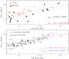 |
Fig. C.1 Size–mass relation for JKCS 041 (top panel, black points), A1689 (top panel, red points), and for five nearby clusters (bottom panel, points) and clusters in Valentinuzzi et al. (2010, blue lines). Both panels report the mean fitted model (solid line) and the 1σ intrinsic scatter (dotted line) for Coma galaxies in Andreon et al. (1996, 1997), our fiducial z = 0 relation. |
Although the data used to construct the z = 0 size–mass relation in Sect. 4.5 are of high quality, the methods used to derive stellar mass and re at z = 0 are not identical to those used in our study of the JKCS 041 members in Paper I. Therefore, it is important to verify that our conclusions are robust to differences in methodology.
Sizes of the Coma members drawn from Andreon et al. (1996, 1997) are based on a curve-of-growth analysis, while the JKCS 041 sizes were instead derived from Sersic fits to the 2D light profiles. However, Aguerri et al. (2004) measured Sersic-based sizes of Coma members and found these to agree with the Andreon et al. (1996, 1997) radii within 10% for the galaxies in common. Furthermore, the Augerri et al. (2004) radii were found to be consistent with later measurements based on HST images using the Advanced Camera for Surveys (Hoyos et al. 2011), which cover a smaller region of Coma but have exquisite depth and resolution. This suggests that the exact method and dataset do not have a strong effect on the sizes at z = 0.
In addition to Coma galaxies, for our z ~ 0 compilation we also drew upon measurements in A1689 at z = 0.189 by Houghton et al. (2012), who assembled a mass-limited sample of early-type galaxies and used Sersic profile fitting to derive re. Furthermore, we included the five nearby clusters studied by Pahre (1999), including Coma, who derived re by fitting seeing-convolved de Vaucouleurs (1948) profiles to K-band imaging. In all cases, we converted from luminosity to stellar mass using our standard BC03 model with zf = 3. For the Pahre data we used the K-band luminosity, while the R-band luminosity was used for the other clusters.
The fit to the size–mass relation in A1689 gives  (C.1)with an intrinsic scatter 0.16 ± 0.03 dex in log re at a given mass. For the Pahre (1999) sample we find
  (C.2)with an intrinsic scatter 0.15 ± 0.01 dex in log re for the full sample (bottom panel of Fig. C.1), and
  (C.3)with an intrinsic scatter 0.16 ± 0.02 dex in log re when Coma is excluded. Figure C.1 demonstrates that these relations are consistent with our fiducial relation derived for Coma based on the Andreon et al. (1996, 1997) measurements. In the lower panel, we also compare this with the size–mass relation from Valentinuzzi et al. (2010) and again find reasonable consistency. To summarize, neither the precise method used to derive mass and re, nor the particular clusters chosen for comparison appear to produce strong effects on the size–mass relation of early-type cluster galaxies at z = 0.
We note that the Shen et al. (2003) size–mass relation for early-type field galaxies in the SDSS, selected using a Sersic index threshold n> 2.5, falls on the upper boundary of the relations plotted in Fig. C.1. Since the present paper is based on the evolution of cluster galaxies, we preferred to use local samples that are confined to cluster members. Furthermore, differences in the morphological distribution of cluster and field galaxies can affect a comparison with the size–mass relation, as discussed in Paper I.
All Tables
All Figures
|
Fig. 1 Completeness of our Y-band imaging of JKCS 041. The Y-band magnitude within a 0.5 arcsec aperture compared with the peak surface brightness. There are galaxies with a peak surface brightness fainter than the detection threshold (~26.5 mag arcsec-2, vertical line), but they are undetectable with these data. Extrapolating the trend seen at brighter magnitudes (slanted solid line), the completeness limit (horizontal dashed line) is 27.15 mag. Owing to uncertainties inherent in this extrapolation, we conservatively adopt a limit that is 0.5 mag brighter, which leads to a limiting magnitude of Y = 26.6. |
| In the text | |
|
Fig. 2 Color−magnitude diagram. Upper panel: JKCS 041 spectroscopic members (solid dots) and all 22.5 <H galaxies within the JKCS 041 area (open dots). The locus of an SSP with zf = 5,3,2.5 is shown for comparison (solid lines, from top to bottom). For clarity, error bars are only shown for Y − H> 1 mag galaxies. Central panel: spectroscopic non-members. Bottom panel: control field galaxies with 22.5 <H< 25 mag. In all panels the JKCS 041 Y-band completeness limit is indicated with a slanted dashed line (Y = 26.6 mag), along with the corresponding H completeness limit (vertical dashed line, H = 25 mag) for the reddest red-sequence galaxies. The JKCS 041 spectroscopic completeness limit of H = 22.5 and the locus of red-sequence galaxies (red dashed corridor) are also shown. |
| In the text | |
|
Fig. 3 Color distribution in the cluster (red) and control field (blue) for all galaxies (top panel), bright galaxies (middle panel) and faint galaxies (bottom panel). Since membership is available on an individual basis for the bright galaxies, no control field is required for the middle panel. Colors are corrected for the slope of the color−magnitude relation assuming a slope of 0.05, consistent with the JKCS 041 data and with slopes observed at z = 0. |
| In the text | |
|
Fig. 4 Luminosity (bottom axis) and stellar mass (top axis) function of red-sequence cluster members. The solid line is the mean model fitted to the individual galaxy data, while the shading indicates the 68% uncertainty (highest posterior density interval). Points and approximated error bars are derived by binning galaxies in magnitude bins, adopting approximated Poisson errors summed in quadrature, as commonly done in the literature. The top axis indicates the corresponding stellar mass, based on our standard BC03 SSP model with zf = 3. |
| In the text | |
|
Fig. 5 Spatial distribution of red-sequence galaxies (red points), with symbols encoding brightness (brighter galaxies are indicated by larger points) and membership (spectroscopic members are indicated by filled points). The four blue spectroscopic members are also shown as blue points. The ellipse indicates the outermost detected X-ray isophote, and the slanted rectangle encloses the full-depth WFC3 field of view. |
| In the text | |
|
Fig. 6 Radial profile of red-sequence galaxies. The solid line is the mean fit and the shading indicates the 68% uncertainty. The control field data point has been arbitrary put at r = 3.6 for clarity. |
| In the text | |
|
Fig. 7 Weighted age distribution of the spectroscopic members of JKCS 041that lie on the red sequence, sorted in order of decreasing mass (more massive toward the top). The three vertical lines correspond to zf = 2.5,3,3.5 Gyr from left to right. |
| In the text | |
|
Fig. 8 Age–mass relation for red-sequence galaxies in JKCS 041. The clouds of colored points show the probability distribution for each individual galaxy, following the color coding in Fig. 7; ellipses show Laplace approximations. The straight solid line is the mean age–mass relation derived from these posteriors, based on the galaxy spectra and photometry. Fan-shaped lines delineate the error on the mean model (68% highest posterior interval), while the dotted lines indicate the intrinsic scatter (±1σ). |
| In the text | |
|
Fig. 9 Size–mass relation for JKCS 041. Lines show the mean fitted model and its uncertainty (solid line and yellow band), along with the intrinsic scatter (dotted line). Points are color-coded according to their location in the age–mass plane (Fig. 7): older (red) or younger (blue) than the mean relation by at least 1σintr, with black points indicating galaxies within ± 1σintr the mean age–mass relation. |
| In the text | |
|
Fig. 10 Comparison of the luminosity function of red-sequence galaxies for JKCS 041 (blue points with large error bars, shading and lines as in previous figure) and Coma (black points; from Andreon 2008). The JKCS 041 LF has been re-normalized to the Coma cluster φ∗ for display purposes only. Labels on the upper x-axis indicate the stellar mass, derived from the H-band magnitude assuming our standard BC03 SSP settings with zf = 3. |
| In the text | |
|
Fig. 11 Faint-end slope of the luminosity function of red-sequence galaxies of 42 clusters spanning over 10 Gyr of the age of the Universe. Top panel: open dots are from De Propris et al. (2013), the open square represents the Crawford et al. (2012) determination, while solid dots are our own work (this work or Andreon 2008 and references therein). Some points indicates stacks of two or ten clusters. The solid line is the mean model, while the shaded area represent the 68% uncertainty (highest posterior density interval) of the mean relation. Bottom panel: as in the top panel, with the amount of ink is proportional to the weight given to each point in the fit. |
| In the text | |
|
Fig. 12 Characteristic magnitude of red-sequence galaxies across 10 Gyr. Locii of constant |
| In the text | |
|
Fig. 13 Size–mass relation for JKCS 041 (black squares) and Coma (red points) galaxies. The figure also presents the mean fitted model (solid line) and the one-sigma intrinsic scatter (dotted line) around the relation for Coma galaxies. |
| In the text | |
|
Fig. 14 68 and 95 % probability contours for JKCS 041 (blue) and Coma (red) size–mass relation. |
| In the text | |
|
Fig. A.1 Implicit prior on the SFH-weighted age tw used in Paper I when fitting galaxy spectra and photometry, arising from the log-uniform priors on t0 and τ. In the present paper we prefer a uniform prior on tw and so have divided out this prior. |
| In the text | |
|
Fig. B.1 Rest-frame λ sampling of the adopted filters for the clusters studied in Bildfell et al. (2012) (z< 0.57). The shaded (yellow) band marks the 4000 Å break. |
| In the text | |
|
Fig. C.1 Size–mass relation for JKCS 041 (top panel, black points), A1689 (top panel, red points), and for five nearby clusters (bottom panel, points) and clusters in Valentinuzzi et al. (2010, blue lines). Both panels report the mean fitted model (solid line) and the 1σ intrinsic scatter (dotted line) for Coma galaxies in Andreon et al. (1996, 1997), our fiducial z = 0 relation. |
| In the text | |
Current usage metrics show cumulative count of Article Views (full-text article views including HTML views, PDF and ePub downloads, according to the available data) and Abstracts Views on Vision4Press platform.
Data correspond to usage on the plateform after 2015. The current usage metrics is available 48-96 hours after online publication and is updated daily on week days.
Initial download of the metrics may take a while.