| Issue |
A&A
Volume 565, May 2014
|
|
|---|---|---|
| Article Number | A1 | |
| Number of page(s) | 19 | |
| Section | Astrophysical processes | |
| DOI | https://doi.org/10.1051/0004-6361/201322969 | |
| Published online | 18 April 2014 | |
Long term variability of Cygnus X-1⋆
VI. Energy-resolved X-ray variability 1999–2011
1
Dr. Karl-Remeis-Sternwarte and Erlangen Centre for Astroparticle Physics
(ECAP), Friedrich Alexander Universität Erlangen-Nürnberg,
Sternwartstr. 7,
96049
Bamberg,
Germany
e-mail:
This email address is being protected from spambots. You need JavaScript enabled to view it.
2
Massachusetts Institute of Technology, Kavli Institute for
Astrophysics, Cambridge
MA
02139,
USA
3
CRESST, University of Maryland Baltimore County,
1000 Hilltop Circle,
Baltimore
MD
21250,
USA
4
NASA Goddard Space Flight Center, Astrophysics Science
Division, Code 661,
Greenbelt
MD
20771,
USA
5
Max-Planck-Institut für Radioastronomie,
auf dem Hügel 69, 53121
Bonn,
Germany
6
Astronomical Institute “Anton Pannekoek”, University of
Amsterdam, Kruislaan
403, 1098 SJ
Amsterdam, The
Netherlands
7
Space Sciences Laboratory, 7 Gauss Way, University of
California, Berkeley
CA
94720,
USA
8
Laboratoire AIM, UMR 7158, CEA/DSM – CNRS – Université Paris
Diderot, IRFU/SAp,
91191
Gif-sur-Yvette,
France
9
Lawrence Livermore National Laboratory,
7000 East Ave., Livermore
CA
94550,
USA
10
Center for Astrophysics and Space Sciences, University of
California San Diego, La Jolla,
9500
Gilman Drive, CA
92093,
USA
11 Alexander von Humboldt fellow
12
Ludwig-Maximilians University, Excellence Cluster
“Universe”, Boltzmannstr.
2, 85748
Garching,
Germany
Received: 1 November 2013
Accepted: 16 February 2014
Abstract
We present the most extensive analysis of Fourier-based X-ray timing properties of the black hole binary Cygnus X-1 to date, based on 12 years of bi-weekly monitoring with RXTE from 1999 to 2011. Our aim is a comprehensive study of timing behavior across all spectral states, including the elusive transitions and extreme hard and soft states. We discuss the dependence of the timing properties on spectral shape and photon energy, and study correlations between Fourier-frequency dependent coherence and time lags with features in the power spectra. Our main results follow. (a) The fractional rms in the 0.125–256 Hz range in different spectral states shows complex behavior that depends on the energy range considered. It reaches its maximum not in the hard state, but in the soft state in the Comptonized tail above 10 keV. (b) The shape of power spectra in hard and intermediate states and the normalization in the soft state are strongly energy-dependent in the 2.1–15 keV range. This emphasizes the need for an energy-dependent treatment of power spectra and a careful consideration of energy- and mass-scaling when comparing the variability of different source types, e.g., black hole binaries and AGN. PSDs during extremely hard and extremely soft states can be easily confused for energies above ~5 keV in the 0.125–256 Hz range. (c) The coherence between energy bands drops during transitions from the intermediate into the soft state but recovers in the soft state. (d) The time lag spectra in soft and intermediate states show distinct features at frequencies related to the frequencies of the main variability components seen in the power spectra and show the same shift to higher frequencies as the source softens. Our results constitute a template for other sources and for physical models for the origin of the X-ray variability. In particular, we discuss how the timing properties of Cyg X-1 can be used to assess the evolution of variability with spectral shape in other black hole binaries. Our results suggest that none of the available theoretical models can explain the full complexity of X-ray timing behavior of Cyg X-1, although several ansatzes with different physical assumptions are promising.
Key words: X-rays: binaries / stars: individual: Cygnus X-1 / binaries: close
Appendix A is available in electronic form at http://www.aanda.org
© ESO, 2014
1. Introduction
The canonical states of accreting black hole binaries have first been observed and defined in the spectral domain: a hard state with a power law spectrum with a photon spectral index of ~1.7 and a soft state with a spectrum dominated by thermal emission from an accretion disk. They are joined by usually short-lived transitional or intermediate states. The whole sequence of states – from hard state over the intermediate into soft, then again into intermediate, and finally into hard state – can best be depicted on a hardness–intensity diagram (HID), where transient sources that undergo a full outburst follow a q-shaped track (Fender et al. 2004, see McClintock & Remillard2006, for a different nomenclature). Radio emission is detected in the hard state, with jets imaged for Cyg X-1 (Stirling et al. 2001) and GRS 1915+105 (Dhawan et al. 2000; Fuchs et al. 2003). In the soft state, radio emission is strongly quenched. Evidence of similar spectral behavior also exists in several other classes of accreting objects, such as neutron star X-ray binaries (e.g., Maitra & Bailyn 2004, Aql X-1), active galactic nuclei (AGN; Körding et al. 2006), and dwarf novae (Körding et al. 2008, SS Cyg).
The spectral states, including the different flavors of the intermediate state, show distinct X-ray timing characteristics, such as shapes of power spectra or time lags between emission at different energies. Timing parameters seem to be a remarkably sensitive tool for defining state transitions (e.g., Pottschmidt et al. 2003; Fender et al. 2009; Belloni 2010).
While the radio emission, and possibly also the gamma-ray emission above 400 keV (Laurent et al. 2011; Jourdain et al. 2012) originate in the jet, the origin of the X-rays is still unclear. As shown, e.g., by Nowak et al. (2011), the combination of the best resolution and the most broadband X-ray spectra available today fails to enable us to statistically distinguish between jet models (Markoff et al. 2005; Maitra et al. 2009) and thermal and/or hybrid Comptonization in a corona (e.g., Coppi 1999, 2004). The fluorescent Fe Kα line and a reflection hump point towards a contribution by reflection, independent of the origin of the continuum (see Reynolds & Nowak 2003; for a review and Duro et al. 2011; Tomsick et al. 2014, and references therein for Cyg X-1).
Spectro-timing analysis holds the promise of solving this ambiguity, since a truly physical model has to consistently describe both spectral and timing behavior. While no self-consistent models that would encompass all parameters exist yet, some studies address, for instance, simultaneous modeling of photon spectra and root mean square variability (rms) spectra (Gierliński & Zdziarski 2005) or photon spectra and Fourier-dependent time lags (Cassatella et al. 2012b). Theoretical ansatzes to describe the X-ray variability include propagating mass accretion rate fluctuations (usually based on Lyubarskii 1997, see, e.g., Ingram & van der Klis 2013, for an analytical model), upscattering in a jet (Reig et al. 2003; Kylafis et al. 2008), and full magnetohydrodynamic simulations (Schnittman et al. 2013, who concentrate on spectra but also address timing properties).
There is mounting evidence for similarities in timing behavior between X-ray binaries, AGN (see McHardy 2010, for a review), and recently also cataclysmic variables (see Scaringi et al. 2013, for discovery of Fourier-dependent time lags). Because of their brightness and short variability timescales, X-ray binaries remain the best laboratories for investigating these phenomena, and they are key to deciphering the complex and currently highly disputed interplay of accretion and ejection processes. We note especially that AGN are usually seen in a single state due to the very much longer variation timescale, and thus X-ray binaries are needed to study the variety of states and their inter-relationships.
The first step to understanding the X-ray timing characteristics is a fundamental overview of their evolution with the spectral shape that can only be achieved with a large number of high quality observations densely covering all states, including the elusive transitions. Most previous works concentrate on energy-independent evolution of rms and power spectral distributions (PSDs) with spectral state (e.g., Pottschmidt et al. 2003; Belloni et al. 2005; Axelsson et al. 2006; Klein-Wolt & van der Klis 2008), although further spectral shape-, energy-, and Fourier frequency-dependent correlations have been noted in individual observations and smaller samples (e.g., Homan et al. 2001; Rodriguez et al. 2002, 2004; Kalemci et al. 2004; Böck et al. 2011; Cassatella et al. 2012a; Stiele et al. 2013), often with a focus on the behavior of narrow quasi-periodic oscillations. Missing are consistent analyses of the energy-resolved evolution of rms and PSDs, Fourier-frequency dependent evolution of cross-spectral quantities (coherence function and lags), and correlations of features in PSDs and in Fourier-frequency-dependent cross-spectral quantities over the full range of spectral states and over multiple transitions. In this paper, we address these questions with an extraordinarily long and well sampled RXTE campaign on the high mass black hole binary Cyg X-1 that enables us to conduct the most comprehensive spectro-timing analysis of a black hole binary to date.
Located at a distance of  kpc (Reid et al. 2011, consistent with Xiang et al. 2011), Cyg X-1 is bright (in the hard state ~7 × 10⁻⁹ erg cm-2 s-1 in the 1.5–12 keV band of RXTE-ASM) and persistent, hence a prime target for both spectral and timing studies. Often considered a prototypical black hole binary, it is frequently used for comparisons with other black hole binaries (e.g, Muñoz-Darias et al. 2010) and AGN (Markowitz et al. 2003; McHardy et al. 2004; Papadakis et al. 2009). Although the spectrum of the source is never fully dominated by the disk and the bolometric luminosity changes by a factor of only ~4 (Cui et al. 1997; Shaposhnikov & Titarchuk 2006; Wilms et al. 2006, and references therein), Cyg X-1 often undergoes state transitions (e.g., Pottschmidt et al. 2003; Wilms et al. 2006; Grinberg et al. 2013) and is therefore also well suited to study the intermediate states.
Here, we analyze data from the 1999–2011 set of RXTE observations of Cyg X-1. This paper is a part of a series where we previously analyzed spectro-timing correlation in the hard state 1998 to 2001 (Pottschmidt et al. 2003), the rms-flux relation (Gleissner et al. 2004b), the radio-X-ray correlations (Gleissner et al. 2004a), the spectral evolution 1999–2004 (Wilms et al. 2006), and states and state transitions 1996–2012 with all sky monitors (Grinberg et al. 2013). We start Sect. 2 by introducing the data and the general behavior of the source during the time period covered by this analysis and follow with a description of the spectral analysis and employed X-ray timing techniques. In Sect. 3, we discuss the energy-independent and -dependent evolution of the rms and the PSDs with spectral shape. In Sect. 4, we discuss the evolution of cross-spectral quantities with spectral shape. We address the implications of our results for the analysis of other sources in Sect. 5 and for theories explaining the origin of X-ray variability in Sect. 6. Section 7 summarizes our finding with a focus on the implied directions for further investigations.
2. Data analysis
The data analyzed here are mostly from a bi-weekly observational campaign with RXTE that was initiated by some of us in 1999 and continued until the demise of RXTE at the end of 2011. Parts of the data have been analyzed in the previous papers of this series (Pottschmidt et al. 2003; Gleissner et al. 2004b,a; Wilms et al. 2006; Grinberg et al. 2013) and by other authors (e.g., Axelsson et al. 2005, 2006; Shaposhnikov & Titarchuk 2006). For all pointed RXTE observations of Cyg X-1 made during the lifetime of the RXTE satellite (MJD 50 071–55 931), we extracted spectral data in the standard2f mode from Proportional Counter Unit 2 of RXTE’s Proportional Counter Array (PCA, Jahoda et al. 2006) and from RXTE’s High Energy X-ray Timing Experiment (HEXTE, Rothschild et al. 1998) on a satellite orbit by satellite orbit basis. The data reduction was performed with HEASOFT 6.11 as described by Grinberg et al. (2013) and resulted in a total of 2741 spectra. At the time of writing there had been no changes to relevant pieces of HEASOFT since this release. We stress the importance of the orbit-wise approach, as spectral and timing properties of Cyg X-1 can change on timescales of less than a few hours (Axelsson et al. 2005; Böck et al. 2011; Grinberg et al. 2013).
2.1. Long-term source behavior
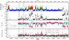 |
Fig. 1 Evolution of Cyg X-1 over the RXTE lifetime. Vertical lines represent the starting times of the RXTE calibration epochs used in this work: dashed line for epoch 3, dot-dashed line for epoch 4, and dot-dot-dashed line for epoch 5. The total ASM count rate is color-coded according to ASM-based state definition of Grinberg et al. (2013), which uses both ASM count rate and ASM hardness of a given measurement: blue represents the hard state, green the intermediate state, and red the soft state. ASM data points after MJD 55 200 are affected by instrumental decline (Vrtilek & Boroson 2013; Grinberg et al. 2013) and shown in gray. The soft photon index Γ1 is shown only for those 1980 RXTE observations that were conducted in the B_2ms_8B_0_35_Q binned data mode, see Sect. 2.3. The rms is calculated in the 0.125–256 Hz range (Sect. 3.1), the time lags are averaged values in the 3.2–10 Hz range (Sect. 4.3). |
The general behavior of Cyg X-1 during the lifetime of RXTE has been discussed by Grinberg et al. (2013). Figure 1 presents an overview of the evolution of the RXTE All Sky Monitor (ASM, Levine et al. 1996) count rate, the spectral shape, and a choice of typically used X-ray timing parameters.
The data used here cover periods of different source behavior, such as pronounced, long hard and soft states, and multiple failed and full state transitions. The strict use of the same data mode means that we do not cover some of the observations included in previous long-term monitoring analyses by Pottschmidt et al. (2003), Axelsson et al. (2005, 2006), or Shaposhnikov & Titarchuk (2006), especially the data from the extreme hard state before 1998 May. The long time span covered in this work that includes the extraordinarily long, hard state of ~MJD 53900–55375 (mid-2006 to mid-2010), and the following series of stable soft states represents, however, a major improvement over all previous analyses.
2.2. Spectral analysis
The spectral analysis presented here is the same as the one we used in Grinberg et al. (2013, Sects. 2.2 and 3.2), so we give only a brief overview. We describe the ~2.8–50 keV PCA data and the 18–250 keV HEXTE data, both rebinned to a signal-to-noise ratio of 10, using a simple phenomenological model that has been shown to offer the best description of RXTE data of Cyg X-1 (Wilms et al. 2006, who also discuss advantages of this model over more physically motivated approaches). The basic continuum model consists of a broken power law with soft photon index Γ1, hard photon index Γ2, and a break energy at ~10 keV. The continuum is modified by a high energy cut-off (Ecut ≈ 20–30 keV, Efold ≈ 100–300 keV, both correlated with Γ1), an iron Kα-line at about 6.4 keV, and absorption, described by the tbnew 1 model, an advanced version of tbabs , with abundances of Wilms et al. (2000) and the cross sections of Verner et al. (1996). An additional soft excess is modeled by a multicolor disk ( diskbb , Mitsuda et al. 1984; Makishima et al. 1986) where necessary, i.e., predominantly in softer observations. A good fit can be achieved with at least one of the two models for all our observations. The disk is accepted as real if the improvement in χ2 is more than 5%, irrespective of the  -value of the model without the disk. This approach ensures a smooth transition between models without and with a disk. The dominance of systematic errors in the lowest channels that define the disk component prevents us from using a significance-based criterion. PCA’s calibration uncertainties are taken into account by adding systematic errors in quadrature to the data (1% added to the fourth PCA bin and 0.5% to the fifth PCA bin in epochs 5 and 4; 1% to the fifth PCA bin and 0.5% to the sixth PCA bin in epoch 3; see Hanke 2011; and Böck et al. 2011).
We identify seven observations where the above χ2 criterion for the model selection results in a preference for the model with a disk but the disk is peculiarly strong and the soft photon index is very steep, making these observations outliers in the tight correlation of Γ1 with ΔΓ = Γ1 − Γ2 (Wilms et al. 2006). The observations can also be clearly seen as outliers in the tight correlation between rms ratio and Γ1 discussed in Sect. 3.1 when Γ1-values of the models with a disk are used. When modeling these seven observations without a disk, all have pronounced residuals at ~5 keV due to the Xe L-edge (Wilms et al. 2006), no signature of a strong disk in the residuals, and an acceptable reduced χ2< 1.3. This behavior indicates that the strong disk component and the steeper soft photon index compensate for the instrumental Xe L-edge and are not an adequate description of the source spectrum. We therefore accept the model without a disk as the best fit model for these observations2. The Γ1-values for these observations shift from the 2.0–2.2 to the 1.8–2.0 range. We emphasize that if the disk were real and not compensating for sharp calibration features, the removal of the disk component would result in an increase of Γ1, contrary to what is seen here.
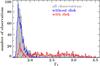 |
Fig. 2 Number of orbit-wise RXTE observations of Cyg X-1 in the B_2ms_8B_0_35_Q mode with a given Γ1. Shown are both observations that require a disk (red) and do not require a disk (blue), and the total number of observations (gray). |
We consider the 1980 spectra for which data in the B_2ms_8B_0_35_Q mode is available (see Sect. 2.3). Our fits yield  for all observations, and a fit with
  can be achieved for 1721 out of these 1980. In the following, we will use Γ1 as a proxy for the spectral state, since all other spectral parameters show strong correlations with Γ1 (Wilms et al. 2006). In particular, in Grinberg et al. (2013) we have defined the hard state as Γ1< 2.0, the intermediate state as 2.0 < Γ1< 2.5, and the soft state as Γ1 > 2.5. Figure 2 shows the number of observations at a given Γ1; we note not only the good coverage of the soft and intermediate states, but also the very high number of observations in the hard state.
2.3. Calculation of X-ray timing quantities
We extracted light curves that are strictly simultaneous with the spectral data. For a consistent treatment of the timing properties, we only used observations in the B_2ms_8B_0_35_Q mode, i.e., binned data with eight bands (channels 0–10, 11–13, 14–16, 17–19, 20–22, 23–26, 27–30, and 31–35) and with an intrinsic time resolution of 2-9 s ≈ 2 ms, resulting in 1980 RXTE orbits. Because this data mode does not include PCU information, light curves can only be extracted from all PCU units that were operating during a particular observation together. Since dead time effects depend on the number of active detectors, we treat each combination of PCUs separately. This approach results in an increase in the number of light curves to 2015, some of them associated with the same spectrum. All analyses in this paper were performed with ISIS 1.6.2 (Houck & Denicola 2000; Houck 2002; Noble & Nowak 2008).
Energy bands used for different RXTE calibration epochs.
In Table 1, we list the channel and energy ranges for the four energy bands that were used throughout this work for calculating the timing properties (bands 3 and 4 combine three channel bands each in order to obtain higher count rates). Most of our data fall into epochs 4 and 5 (Fig. 1). The energy range covered by the bands is slightly time dependent because of changes in the high voltage of the PCA, but such small changes will not influence the qualitative analysis presented in this work:
-
Band 1 (2.1–4.5 keV) covers the range with a significant contribution from the accretion disk, which can dominate this band in the soft states. At the high soft count rates of the soft states, this band can suffer from telemetry overflow (Gleissner et al. 2004b; Gierliński et al. 2008), resulting in artifacts at high frequencies above ~30–50 keV as can be seen, e.g., in Fig. A.2 for Γ1 ~ 2.61 and ~2.713.
-
Band 2 (4.5–5.7 keV) covers the soft part of the spectrum above the main contribution of the disk. The band is below the prominent Fe Kα-line at ~6.4 keV, but since the line is broad its contribution may be significant (Wilms et al. 2006; Shaposhnikov & Titarchuk 2006; Duro et al. 2011).
-
Band 3 (5.7–9.4 keV) includes the Fe Kα-line and covers the spectrum up to the spectral break at ~10 keV.
-
Band 4 (9.4–15 keV) mainly covers the spectrum above the spectral break at ~10 keV and below the high-energy cut-off.
We calculated all timing properties (power spectra [power spectral densities, PSD], cross power spectra, coherence, and time lags) following Nowak et al. (1999a) and Pottschmidt et al. (2003). For the timing analysis, each light curve was split into segments of nbins = 4096 bins, i.e., 8 s length. Timing properties were calculated for each segment and then averaged over all segments of a given light curve using the appropriate statistics. The mean number of segments used was ~225, and the mean light curve length therefore ~30 min. Before rebinning, the values of all timing properties were calculated for discrete Fourier frequencies fi linearly spaced every Δf = 1/(nbinsΔt) = 0.125 Hz. The Nyquist frequency of the data is fmax = 1/(2Δt) = 256 Hz, and the lowest frequency accessible is fmin = 1/(nbinsΔt) = 0.125 Hz; i.e., we cover slightly over three decades in temporal frequency. As shown by Nowak et al. (1999a), for a source such as Cyg X-1 and using the approach described above, the dead-time-corrected, noise-subtracted PSDs are reliable to at least 100 Hz. The systematic uncertainties for the coherence function are negligible below 30 Hz, and the phase and time lags are detectable in the 0.1–30 Hz range (Nowak et al. 1999a, but see also Sect. 4.1).
Longer individual segments would enable us to probe lower Fourier frequencies. The lower number of averaged segments per observation would mean higher uncertainties, but generally still reliable results in the case of PSDs. Coherence function and lags are, however, higher order derivative statistics and therefore more sensitive to uncertainties. Thus, to constrain them well, a larger number of segments is necessary; i.e., the individual segments have to be shorter.
For PSDs, we choose the normalization of Belloni & Hasinger (1990) and Miyamoto et al. (1991), where the PSD is given in units of the squared fractional rms variability per frequency interval. Since the variance that each frequency contributes is given in units of average signal count rate, this normalization is most suitable for comparing PSD shapes independently of source brightness (Pottschmidt 2002). To illustrate the contribution of the variability at a given Fourier frequency, fi, to the total variability, we show the PSDs in units of PSD times frequency, PSD(fi) × fi (Belloni et al. 1997; Nowak et al. 1999a). We calculated the fractional rms by summing up the contributions at individual frequency ranges without employing any modeling of the PSD shape; all rms values in this work are given for the 0.125–256 Hz range.
While the PSD describe the variability of one light curve, the relationship between two simultaneous light curves can be characterized by the cross spectral density. Such a cross spectrum is calculated as a product of the Fourier transform of one light curve with the complex conjugate of the Fourier transform of the other light curve.
The coherence function, γ2(fi), a derivative of the norm of the cross spectrum, measures the Fourier-frequency dependent degree of linear correlation between two time series, in this case the light curves (Vaughan & Nowak 1997). An intuitive geometrical interpretation of γ2(fi) as a length of a vector sum in the complex plane can be found in Nowak et al. (1999a).
For two correlated time series, we can define the Fourier-frequency dependent phase lag φi at a frequency fi as the difference between the phases of the Fourier transforms of the light curves in both energy bands, calculated as the argument of the complex cross spectrum. The time lag at the frequency fi is then given by δt(fi) = φi/ (2πfi). Our sign convention is such that the hard light curve lags behind the soft for a positive lag. Since the phase lag, φ, is defined on the interval [−π,π [, there is an upper limit for absolute value of the time lag. Experience shows that the lags are below this limit in the considered frequency range in objects such as Cyg X-1 (e.g., Nowak et al. 1999a; Pottschmidt et al. 2000, 2003; Böck et al. 2011), Swift J1753.5−0127 (Cassatella et al. 2012a), or XTE J1752−223 (Muñoz-Darias et al. 2010).
3. Rms and power spectra
3.1. Evolution of fractional rms with spectral shape
We start with the most basic quantity, the rms variability of the source. As we have previously shown (Grinberg et al. 2013), the total fractional rms in the 0.125–256 Hz frequency band strongly depends on the spectral state and on the energy band. Here, we analyze this behavior in more detail.
3.1.1. Energy-independent vs. energy-dependent evolution of rms
Figure 3 shows how the fractional rms in the 2.1–15 keV band depends on the spectral shape. Here and in the following sections, the errors of the rms are expected to be smaller than the spread of the shown correlations at any give Γ1. The rms reaches its highest values of ~34% at the lowest Γ1 of ~1.6. The Γ1-rms correlation is negative below Γ1 ≈ 1.8, then flat until Γ1 ≈ 2.0, again negative until Γ1 ≈ 2.5–2.7, and finally flattens out at an rms of ~20% but with a larger scatter.
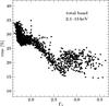 |
Fig. 3 Fractional rms in the 2.1–15 keV band vs. soft photon index Γ1. |
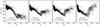 |
Fig. 4 Fractional rms in the 0.125–256 Hz frequency band for different energy bands vs. the soft photon index, Γ1, of the broken power law fits. |
The energy-dependent fractional rms reveals where most of this variability in the total 2.1–15 keV band comes from in the different spectral states. Figure 1 shows the temporal evolution of the fractional rms in the soft band 1 and the hard band 4 (2.1–4.5 keV and 9.4–15 keV) over the lifetime of RXTE. During hard states, the variability is high at about ~30% in both bands. In the soft state, the rms drops to 10–20% in band 1, but in band 4 it is slightly larger than in the hard state. The intermediate state is associated with a decrease in rms in both bands. This behavior is better visualized in Fig. 4, where we plot rms as a function of Γ1 for bands 1–4. By eye, we identify four Γ1 ranges with different behavior (see Table 2 for correlation coefficients for bands 1–4 and the total band).
-
Γ1< 1.8: the Γ1–rms correlation is negative and becomes stronger at higher energies in the individual and the total bands;
-
1.8 ≤ Γ1< 2.0: the correlation is positive for bands 1 and 2 and negative for band 4. In band 3, the rms values are consistent with being uncorrelated with Γ1, an understandable behavior given the change of sign in adjacent bands. In the total band, there is no correlation;
-
2.0 ≤ Γ1< 2.65: the correlation is strong and negative in all bands including the total, though it becomes less steep with increasing energy;
-
2.65 ≤ Γ1: the correlation changes from negative in band 1 (note the negative ρ-value in Table 2) to positive in bands 2–4 and becomes stronger with increasing energy. The total rms in the 2.1–15 keV band shows no correlation with spectral shape. There is a slight indication of further structure at Γ1 ~ 2.8–2.9 in energy bands 2–4.
The changes in slope of the rms-Γ1 relationship at Γ1 ~ 1.8 and Γ1 ~ 2 are present both when considering only observations that do not require a disk and only observations that do require a disk. These changes are therefore not artifacts caused by the choice of spectral model used to measure Γ1. For Γ1 > 2, the number of observations that do not require a disk is negligible (Fig. 2). We also note that the Γ1 thresholds represent approximate values, since the transition from one behavior pattern to the other is not clearly defined.
Spearmann ρ correlation coefficients for Γ1–rms correlation.
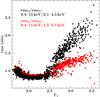 |
Fig. 5 Ratio of fractional rms in different energy bands (band 1 – rms1, band 2 – rms2, band 4 – rms4,) vs. soft photon index Γ1. |
A compact representation of the rms behavior is given by the ratio of the rms values between the different bands (Fig. 5). The relation is tight enough that it can serve as a simple check for the spectral shape of the source without any model assumptions. We used it, for example, to check our broken power law fits for outliers as described above in Sect. 2.2. We emphasize that because of the strong energy dependence of the rms, the total fractional rms in the 2.1–15 keV band (Fig. 3) cannot be used to determine whether one soft state observation is softer than another in terms of relative Γ1, while the rms at energies above ~6 keV or the ratio of rms at different energies (Fig. 5) can.
The energy-independent analyses of RXTE data by Pottschmidt et al. (2003), who use the 2.1–15 keV range, and Axelsson et al. (2006), who use the 2–9 keV range, are consistent with the rms evolution presented here, although different time ranges are covered. A decrease in the rms as the source softens was also observed at higher energies, namely in the 10–200 keV range using Suzaku-PIN and Suzaku-GSO by Torii et al. (2011) and in the 27–49 keV band using INTEGRAL-SPI by Cabanac et al. (2011), although neither of them observed a full soft state with Γ1 ≳ 2.5, where our analysis shows an increase in the rms above ~6 keV.
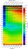 |
Fig. 6 Evolution of fractional rms between 0.125–256 Hz in the eight binned channels of the B_2ms_8B_0_35_Q mode with the X-ray spectral shape represented by the soft photon index Γ1. Black horizontal lines are photon indices for which no data are available. |
To better understand the behavior of rms with both energy and spectral shape, we looked at the behavior of these quantities in the eight bands of the B_2ms_8B_0_35_Q mode (Fig. 6). For each energy band, we determined the average fractional rms from all observations during which a similar photon spectral shape was found. Two photon spectra are considered to be similar if their respective Γ1 values fall into the same bin of a linear grid with steps of ΔΓ1 = 0.01 between Γ1,min = 1.64 and Γ1,max = 3.59. The trends shown in Fig. 4 and Table 2 are confirmed. The higher energy resolution allows us to see the gradual increase in fractional rms with Γ1 for Γ1 ≳ 2.7 at all energies above 4.5 keV. The increase steepens at higher energies. For 1.8 < Γ1< 2.3, the variability is lower above 4.5 keV than below that energy, but the decrease in rms with energy does not appear smooth and shows an indication of recovery above 11 keV.
Examples of rms spectra shown by Gierliński et al. (2010) agree with Fig. 6, but these authors do not observe an increase in the rms above 11 keV for 1.8 < Γ1< 2.3. Such an increase is present (but not pointed out) in the one Cyg X-1 rms spectrum shown by Muñoz-Darias et al. (2010). In the 10–200 keV range, Torii et al. (2011) show that the fractional rms spectra remain largely flat in hard and intermediate4 states and that the intermediate state shows less variability than the hard state; i.e., the behavior presented here for the 2.1–15 keV range continues at higher energies.
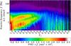 |
Fig. 7 Evolution of PSDs in 2.1–15 keV band (sum of bands 1–4 and full energy range of the B_2ms_8B_0_35_Q mode) with spectral shape. The color scale represents averaged PSD(fi) × fi values at individual Fourier frequencies fi. In this and in all following figures, black vertical lines are photon indices for which no data are available. |
3.2. Evolution of PSDs with spectral shape
Having discussed the overall source variability by studying the rms, we now turn to the Fourier frequency-dependent variability. For our analysis of the change of PSD shapes with spectral state, we choose an approach that does not require us to model the PSDs and thus does not introduce any assumptions on identification of possible components in individual PSDs and their evolution. For possible pitfalls of such assumptions, see Sect. 5.2.
We visualize the evolution of the PSD components as a color map in fi–Γ1-space following an idea of Böck et al. (2011). As in the analysis of the rms behavior, we define a grid with steps of ΔΓ1 = 0.01 between Γ1,min = 1.64 and Γ1,max = 3.59 and 100 equally spaced steps in logarithmic frequency between 0.125 Hz and 256 Hz. When mapping linear Fourier frequencies to this logarithmic grid, some bins remain empty. We allocate these to adjacent bins containing at least one Fourier frequency, equally divided between higher and lower bins. In the following, we first discuss the energy-independent behavior of the power spectra in Sect. 3.2.1, and then turn to the energy-dependent variability in Sect. 3.2.2.
3.2.1. Energy-independent evolution of PSDs with spectral shape
Most previous works address the timing quantities in an energy-independent way. Because of the strong changes in spectral shape (see Nowak et al. 2012, for examples of broadband spectra of Cyg X-1 in hard and soft states) and hence count rate ratios at different energies, extrapolation from energy-band dependent quantities to the full energy range across all spectral states is nontrivial. Thus, we first address the full 2.1–15 keV range and show the evolution of these PSDs with spectral shape in Fig. 7.
For 1.75 < Γ ≲ 2.7, two strong variability components are present. Previous work has shown that such components can be modeled well as (often zero-centered) Lorentzians (e.g., Nowak 2000), and by visual comparison we can identify the components with the two Lorentzians of Böck et al. (2011) and with the two lowest frequency Lorentzian components of Pottschmidt et al. (2003). In the spirit of the approach chosen here that avoids depending on models for the variability, we label the lower frequency variability component as component 1 and the higher frequency variability component as component 2. Both components shift to higher frequencies as Γ1 softens (see also Cui et al. 1997; Gilfanov et al. 1999; Pottschmidt et al. 2003; Axelsson et al. 2005; Shaposhnikov & Titarchuk 2006; Böck et al. 2011). The two components appear to have roughly similar strengths. In the PSDs shown in the 2.1–15 keV band, we observe that component 2 disappears at Γ1 ≈ 2.5, so that the PSD is dominated by component 1 for 2.5 < Γ1< 2.7. We also draw attention to the low variability at the lowest frequencies in the Γ1 ~ 2.3–2.6 range. At the highest frequencies, the PSDs in all Γ1-ranges are dominated by low statistics and therefore noise.
For Γ1 ≲ 1.75, we see additional power at frequencies above ~2 Hz, i.e., above the frequencies assumed by components 1 and 2 in this Γ1-range. This behavior is consistent with the appearance of the third Lorentzian component in the very hard observations analyzed by Pottschmidt et al. (2003) and Axelsson et al. (2005). We note that the hardest observations analyzed by these authors are from before 1998 April, i.e., during a time not covered by the data mode we use, while the hardest spectra analyzed here were observed during the long hard state between mid-2006 and mid-2010 (Nowak et al. 2011; Grinberg et al. 2013). Interestingly, the overall variability amplitude increases in this Γ1-range at all frequencies below ~10 Hz.
For Γ1 ≳ 2.7, the variability is generally low, consistent with low total rms in this range (Fig. 3). It is continuous, without pronounced components, and strongest at the lowest frequencies and decreases towards higher frequencies.
3.2.2. Energy-dependent evolution of PSDs with spectral shape
The energy-dependent evolution of the fractional rms (Sect. 3.1) hints at the PSDs being highly dependent on the energy band considered, especially in the soft spectral state. The shape of the PSDs in all four energy bands is shown in Fig. 8. These maps emphasize the dominant components and use a linear color scale for the PSD(fi) × fi values, while usually individual power spectra are presented on a logarithmic PSD(fi) × fi-axis (Figs. A.1−A.4).
For 1.75 ≲ Γ1 ≲ 2.7, we observe the same two variability components as in the energy-independent PSDs. Both components become weaker with increasing energy. The amplitude of component 1 decreases faster than the amplitude of component 2: component 1 is stronger than component 2 in band 1 (4.5–5.7 keV), but in band 4 (9.4–15 keV) component 2 is more pronounced. Especially in the Γ1 ≈ 2.4–2.6 range, component 1 dominates the lower energy bands, but component 2 the higher energy bands.
For Γ1 ≲ 1.75, the shape of the PSDs appears energy-independent, as opposed to the softer observations. The additional higher frequency component discussed in Sect. 3.2.1 is present in all bands.
For Γ1 ≳ 2.7, the variability shows a behavior that is fundamentally different from the behavior of the two components in the 1.75 ≲ Γ1 ≲ 2.7 range, as already indicated by the different behavior of the rms in Sect. 3.1. In band 1, the overall variability is low, consistent with the evolution of the total rms. What variability there is seems to show a slight trend towards lower frequencies with increasing Γ1 (see also Fig. A.3). In bands 2 to 4, the variability increases strongly with increasing energy of the band and within an energy band with increasing Γ1.
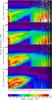 |
Fig. 8 Evolution of the PSDs with spectral shape represented by the soft photon index Γ1 of the broken power law fit in four energy bands (see Table 1). The color scale represents averaged PSD(fi) × fi values at individual Fourier frequencies fi. |
Figures A.1–A.4 present average PSDs at different spectral shapes to facilitate comparison with previous work. While the continuous change in the PSD is better illustrated in the approach of Fig. 8, two effects are better represented by looking at fi-PSD(fi) × fi-plots of PSDs. First, in the frequency range considered here, the power spectra at energies above ~5 keV are similar for the hardest observations with Γ1< 1.75 and the softest observations with Γ1 > 3.15, as can be easily seen on Figs. A.1–A.4 and as shown for two example Γ1 values in Fig. 9. While the different dependence of the PSDs themselves on the energy and the different cross-spectral properties (see Sect. 4) suggest a different origin for these power spectra, the shapes can easily be confused, especially when data are of lower quality. Secondly, there are indications of a weak third hump above 10 Hz for 1.75 ≲ Γ1 ≲ 2.15 that is not visible in this range in Fig. 8 and that corresponds to the higher frequency Lorentzian component L3 modeled by Pottschmidt et al. (2003). For the hardest observations with Γ1 ≲ 1.75, there are also hints of a further component at ~30 keV (see also Revnivtsev et al. 2000; Nowak 2000; Pottschmidt et al. 2003).
An energy-dependent approach to both rms and PSDs is clearly necessary for understanding the variability components in different states because they show strikingly different behavior with the changing energy, which is otherwise missed. This result may be especially important when comparing black hole binaries to AGN and cataclysmic variables, where at the same energy we probe different parts of the emission (see also Sect. 5.3).
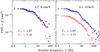 |
Fig. 9 Comparison of average PSDs for Γ1 ~ 1.67 (blue stars) and Γ1 ~ 3.49 (red squares). PSDs are calculated for a logarithmically binned grid with df/f = 0.15. Each PSD is the average of all n PSDs falling within the Γ1 ± 0.01 interval for the given Γ1 values. Left: band 2 (5.7–9.4 keV). Right: total band (2.1–15 keV). |
3.2.3. Discussion of PSD shapes
The frequency shift of the variability components of the PSDs in the RXTE range with the softening of the source in the hard and intermediate states continues at higher energies (Cui et al. 1997; Pottschmidt et al. 2006; Cabanac et al. 2011) up to ~200 keV (Torii et al. 2011), even though such high energy analyses are rare. The different energy dependence of the components has been previously noted for individual observations, both for the presented energy range and above (Cui et al. 1997; Nowak et al. 1999a; Pottschmidt et al. 2006; Böck et al. 2011), but never shown for such a comprehensive data set as presented in this work.
The ~f-1-variability of the soft state PSDs can be described by a power law, while the power spectra of intermediate states are often modeled with a combination of Lorentzian components with (cut-off) power law (e.g., Cui et al. 1997; Axelsson et al. 2005, 2006). Cui et al. (1997) have noted that the power law component becomes stronger with increasing energy for individual soft state observations up to 60 keV; we observe this effect, which has also been noted by Churazov et al. (2001), up to our maximum energy of 15 keV. We also clearly see that at energies above 4.5 keV the variability grows with increasing Γ1 for Γ1 > 2.7, but decreases below 4.5 keV.
Our approach does not allow us to track the weak power law in the intermediate state, especially given that our lowest accessible frequency is 0.125 Hz. However, we see that the power law dominates the PSDs for Γ1 ≳ 2.7 – the abrupt change can also be seen in the cross spectral quantities presented in the next section (Sect. 4). In particular, for Γ1 ≳ 2.7, the coherence, which shows a dip for 2.5 < Γ1< 2.7, recovers (Sect. 4.1); the time lag spectra lack the previously present structure (Sect. 4.2); and the averaged time lags show an abrupt drop and no correlation with Γ1 for Γ1 ≳ 2.65 (Sect. 4.3). Cross-spectral quantities are thus clearly crucial for gaining a better understanding of the variability of the source and are discussed in the following section.
4. Coherence and time lags
4.1. Evolution of Fourier-dependent coherence with spectral shape
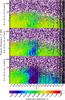 |
Fig. 10 Evolution of the coherence, γ2, with spectral shape represented by the soft photon index Γ1 of the broken power law. The color scale represents averaged γ2 values at individual Fourier frequencies fi. Upper panel: |


We calculate maps of the coherence function,  where h ∈ { 4,3,2 } is the harder band and s ∈ { 3,2,1 } is the respective softer band, using the same grid as in our analysis of the power spectra (Sect. 3.2). Figure 10 shows maps of the coherence function between band 4 and bands 1–3. By eye, we can identify an envelope in all shown coherence functions that follows the high frequency outline of the dominant variability components of the power spectra (Sect. 3.2). Outside of this envelope, the coherence fluctuates strongly.
To assess whether the envelope is an intrinsic feature of the source or whether it is due to the low signal at the high frequencies, we simulate example light curves with typical spectra and PSDs for different values of Γ1. To do so, we use Monte Carlo simulation with the software package SIXTE (SImulation of X-ray TElescopes) developed for the analysis of various X-ray instruments (Schmid 2012). For each selected PSD provided in the SIMulation inPUT (SIMPUT) file format5, the simulation software obtains a light curve using the algorithm of Timmer & König (1995). Here, we use the PSDs in the full 2.1–15 keV band as input PSDs. Based on this light curve, a sample of X-ray photons is generated with the Poisson arrival process generator of Klein & Roberts (1984). The energies of the photons are distributed according to the observed spectrum, which is chosen as constant throughout the simulation. The photons are then processed through a model of the PCA taking instrumental effects into account, such as energy resolution and dead time. The output of this model is a list of simulated events as detected with the PCA, which is converted back to light curves in chosen channel or energy bands for the subsequent analysis. As the spectral shape remains unchanged and only the rate of generated photons, i.e., the normalization of the spectrum, varies with the light curve, the variability in different energy bands is, by definition, coherent.
We simulate light curves in bands 4 and 1 and calculate  as for observed light curves. The trends we observe in are the same as for observed light curves: the coherence function is ~1 below approximately 10 Hz and then shows strong variations above that frequency. This threshold frequency weakly depends on state and decreases towards lower frequencies in the soft state. We therefore conclude that the envelope seen in the coherence function plots is not source-intrinsic but a consequence of the low signal at higher frequencies.
A feature not present in our simulations of ideally coherent light curves is the decrease in coherence for 2.35 ≲ Γ1 ≲ 2.65 in a region that seems to follow the shape of the PSD components 1 and 2 (see Sect. 3.2.1). This decrease is most evident in  , where the coherence values drop below 0.85, but is also visible in
  and indicated in
  (Fig. 10).
For Γ1 ≳ 2.65, the coherence recovers, although the values between the 9.4–15 keV and 2.5–4.5 keV bands remain significantly lower (~0.92–0.94) than between 9.4–15 keV and the 4.5–5.7 keV and 5.7–9.4 keV bands. The coherence seems also noisier, although this is likely due to the lower number of observations in the soft state.
4.2. Evolution of Fourier-dependent time lags with spectral shape
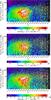 |
Fig. 11 Evolution of time lags δt in the |

The time lags show a strong power law dependence on the Fourier frequency with  (Nowak et al. 1999a, and references therein), so that we consider the fraction
  to visualize structures in the time lag spectra and again follow the approach from Sect. 3.2. In Fig. 11, we present maps of Δδt for band combinations showing the largest lags, i.e., bands with largest separation in energy (Miyamoto et al. 1988; Nowak et al. 1999a). In the phase lag representation, the largest lags between the 2.1–4.5 keV and 9.4–15 keV bands do not exceed ~0.5 rad, so that the time lags are well defined, and the features in Fig. 11 are not due to the phase lag to time lag conversion (see Sect. 2.3).
If the lags strictly followed , then the only structure Δδt would show would be a gradient with changing Γ1, corresponding to the known changes in average lag with state (e.g., Pottschmidt et al. 2003). Such a gradient is indeed visible, with the lags obtaining highest values at Γ1 ~ 2.5–2.6.
For Γ1 ≲ 2.7, however, there is a fi-dependent structure overlaid on the Γ1-dependent gradient. This structure seems to track the two components 1 and 2 of the PSDs (see Sect. 3.2) and is visible for all energy band combinations. A correlation between the features of the PSDs and of time lag spectra has been suggested in Cyg X-1 by Nowak (2000), but to our knowledge has not been shown for a wide range of spectral states and therefore PSD shapes for any black hole binary previously.
For Γ1 ≳ 2.7, the lag spectrum shows no structure and has lower values than for harder Γ1. No evolution with Γ1 is seen in the soft state.
For Γ1< 1.75, where the PSDs show increased variability and a possible additional component at higher frequencies, no corresponding changes can be seen in the Δδt maps. The two components 1 and 2 of the hard and intermediate state PSDs are, however, clearly visible in the time lag maps.
4.3. Evolution of average time lag with spectral shape
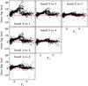 |
Fig. 12 Averaged time lag in the 3.2–10 Hz range vs. soft photon index of the broken power law fits Γ1 for all combinations of energy bands (band 1: 2.1–4.5 keV, band 2: 4.5–5.7 keV, band 3: 5.7–9.4 keV, band 4: 9.4–15 keV). Zero time lag is represented by the dashed red line. |
The usual measure for time lags in the literature are averaged lags δtavg in the 3.2–10 Hz band (e.g., Pottschmidt et al. 2003; Böck et al. 2011). To facilitate comparisons, we follow the approach of the previous work: we rebin each raw time lag spectrum to a logarithmically spaced frequency grid with df/f = 0.15 and then calculate an average value for the 3.2–10 Hz band.
The average time lags (Fig. 12) are larger for bands with a greater difference in energy, but all combinations of energy bands show the same nonlinear trends with Γ1: a strong increase in the time lags from hard to intermediate states and an abrupt drop at Γ1 ~ 2.65 that has also been noted by, e.g., Pottschmidt et al. (2000) and Böck et al. (2011).
Spearman rank coefficients between the average time lag, δtavg, and the soft photon index, Γ1, for Γ1< 2.65 and Γ1 ≥ 2.65 are listed in Table 3. In all bands, δtavg is strongly positively correlated with Γ1 for Γ1< 2.65 and not correlated or weakly negatively correlated with Γ1 for Γ1 ≥ 2.65. The weak negative correlation may be an artifact of the choice of threshold Γ1-values of 2.65. Spearman rank coefficients and their low null hypothesis probabilities do, however, not imply a linear correlation: the relationship for Γ1< 2.65 appears nonlinear, with a bend at Γ1 ~ 1.8–1.9 and a stronger than linear increase towards higher Γ1 (Fig. 12, especially time lag between bands 4 and 1).
4.4. Comparison with previous results for coherence and lags
Cross-spectral analysis is generally less present in the literature, and an analysis of the Fourier-dependent coherence function and time lags for Cyg X-1 across the full range of spectral states of the source is undertaken in this paper for the first time. However, the available previous results agree well with the long-term evolution presented here, in particular for coherence in different spectral states (Cui et al. 1997; Pottschmidt et al. 2003; Böck et al. 2011) and for average time lags in hard and intermediate states (Pottschmidt et al. 2003; Böck et al. 2011). The return to low values in the soft state has been noted before (Pottschmidt et al. 2000; Böck et al. 2011), but the abruptness of the change with Γ1 can only be seen for an extensive data set, such as the one presented here, or for the extremely rare, almost uninterruptedly covered transitions such as the one analyzed by Böck et al. (2011).
In a different approach, Skipper et al. (2013) compute the cross correlation function between the photon index and the 3–20 keV count rate of Cyg X-1 and find different shapes in dim hard states, bright hard states, and soft states. All their hard state cross correlation functions show asymmetries that can only be explained if a part of the hard count rate lags the soft, consistent with our observations of a hard lag. Their dim hard states correspond to the hardest states observed by Pottschmidt et al. (2003) in 1998. These hardest states are similar to our data falling into the Γ1< 1.8 range, i.e., mostly data from the long hard state 2006 to 2010 (Nowak et al. 2011; Grinberg et al. 2013), and therefore before the first bend of the δtavg–Γ1 correlation (Sect. 4.3). Data taken during these states include further components in the PSD, which can also be seen in the hardest observations presented here. Similar evidence of growing hard lags as the source transits into the intermediate state was also found by Torii et al. (2011) in cross correlation function of the 10–60 keV and 60–200 keV Suzaku light curves.
The double-humped structure in the phase lag spectra of Cyg X-1 (Sect. 4.2, for Γ1 ≲ 2.7) has been suggested since the late 1980s (Miyamoto & Kitamoto 1989). Correlated features in the PSDs and time lag spectra were noted for individual observations (Cui et al. 1997; Nowak 2000), but there has been only little work on the systematic evolution of these features with spectral state. We stress the importance of this approach by comparing our results to Pottschmidt et al. (2000), who discuss time lag spectra for individual observations in different states and argue on their basis for a similar shape of the time lag spectra in hard and soft states. While the f-0.7-behavior is indeed dominant in both states and individual hard and soft observations therefore appear similar, we see features correlated with PSD components in the hard but not in the soft state (Fig. 11).
5. Using the variability of Cyg X-1 as a template for other black holes
Before discussing possible implications of the observed variability patterns on physical interpretations of the variability in Sect. 6, we first address the importance of our model-independent approach for long-term timing analysis and the implications for the interpretation and further analysis of variability components in other sources.
5.1. Cyg X-1 and the canonical picture of states and state transitions
A comprehensive analysis of all sources observed with RXTE is out of the scope of this work. In contrast to most transient black hole binaries (see, e.g., Klein-Wolt & van der Klis 2008, for a sample study) and most notably the canonical X-ray transient GX 339−4 (Belloni et al. 2005), Cyg X-1 does not show strong narrow quasi periodic oscillations (QPOs)6, although there is evidence of short-lived QPOs (Pottschmidt et al. 2003, Remillard, priv. comm.). Common for black hole binaries, however, seem to be the two flavors of the hard state with different X-ray timing properties (e.g., Cassatella et al. 2012a, for Swift J1753.5−0127; and Done & Gierliński 2005, for XTE J1550−564), the frequency shift of the main variability components in the hard and intermediate states (e.g, Klein-Wolt & van der Klis 2008), and the sharp change in timing behavior as the source transits into the soft state (e.g., Nowak 1995; Klein-Wolt & van der Klis 2008), all shown here in unprecedented detail for Cyg X-1.
In the canonical picture of the black hole binary states, the rms drops to a few percent in the soft state (Belloni 2010). The rms of Cyg X-1 does not assume such low values, even when the 2.1−4.5 keV band is considered (Fig. 3). However, Cyg X-1 is not the only source showing such behavior: for example, a complex, energy-dependent rms behavior in the soft state with the rms remaining flat in the 3.2–6.1 keV band and increasing in the 6.1–10.2 keV band has also been observed in the 2010 outburst of MAXI J1659−152 (Muñoz-Darias et al. 2011), a source that, like Cyg X-1, does not show a purely disk-dominated soft state. Similar to Cyg X-1, MAXI J1659−152 also shows increased time lags in the intermediate state (Muñoz-Darias et al. 2011). Correlated features in power and time lag spectra were also seen in, e.g., GX 339−4 (Nowak 2000) and Swift J1753.5−0127 (Cassatella et al. 2012b).
5.2. The identification of the variability components
Assuming that we can use Cyg X-1 as a template for the long-term variability of PSDs and cross-power quantities in other black hole binaries, we can avoid misidentification of PSD components in the different spectral states. This is often a problem in observations that are less well sampled than desirable and therefore do not allow tracking the frequency dependency of components in the PSDs with spectral shape. We note, however, that as a persistent source, Cyg X-1 may not cover some of the extreme behavior of the transient sources.
For example, in their study of a state transition of XTE J1650−500, Kalemci et al. (2003) model the power spectrum in the intermediate state as a Lorentzian, which shifts to a higher frequency when comparing the power spectra taken from the 3–6 keV and the 6–15 keV data. A comparison with Fig. 8 shows that the observations of Kalemci et al. (2003) could be explained if this source falls in the spectral range where the lower energy bands are dominated by component 1 and the higher energy bands by component 2 (2.4 ≲ Γ1 ≲ 2.7 for Cyg X-1).
A comparison with Figs. 7 and 8 also reveals a different interpretation of the RXTE observations of Swift J1753.5−0127. Here, Soleri et al. (2013) see two broad peaks that decrease in frequency with increasing spectral hardness, and then jump again to higher frequencies for the hardest observations. The overall pattern seen in our Cyg X-1 data suggests the alternative interpretation that for softer observations the model of Soleri et al. (2013) tracks components 1 and 2, while for the harder observations, the model picks up the prominent component 3 that appears at higher frequencies than components 1 and 2 in our hardest observations (see also Pottschmidt et al. 2003).
5.3. Variability in black hole binaries and AGN
Since the physics of accretion is expected to be similar for compact objects of different mass, the characteristic frequencies seen in the power spectra are expected to scale with mass. AGN are therefore expected to show timing behavior similar to black hole binaries, albeit at higher timescales of hours to years (McHardy et al. 2006). Timing analysis of AGN is, however, notoriously complicated because of the low fluxes and the low frequencies, which are hard to sample well.
PSDs of AGN generally suffer from lower signal-to-noise and sparser sampling than those of black hole binaries, and they are usually modeled with either power laws or broken/bending power laws (see, e.g., González-Martín & Vaughan 2012,for analysis of a large sample observed with XMM-Newton). More complex model shapes with two bends (going to a power-law slope of 0 at the lowest temporal frequencies) or two Lorentzians have only been fit in one case so far, namely Akn 564 (McHardy et al. 2007)7. AGN generally show high coherence that drops at higher frequencies and Fourier frequency- and energy-dependent time lags (Vaughan et al. 2003; Markowitz et al. 2007; Sriram et al. 2009). In Akn 564, the time lag spectra show features at frequencies corresponding to changes in the components dominating the PSD (McHardy et al. 2007). On short timescales, AGN show soft lags between energy bands dominated by soft excess and the power law (e.g., Fabian et al. 2009; De Marco et al. 2013), but we note that the mass-scaled frequency range covered by these observations is not accessible for lag studies in X-ray binaries8. Although they differ in details, the correlations between spectral and timing parameters in AGN and binaries also seem to follow similar trends (Papadakis et al. 2009) and appear to be at least comparable.
As we have seen above (Sects. 3.2.2 and 5.1), PSD shapes in Cyg X-1 and other black hole binaries are, however, strongly energy-dependent. The energy dependence of AGN PSDs has not been studied as well, but relatively higher energy PSDs tend to show either higher break frequencies (e.g., McHardy et al. 2004; Markowitz et al. 2007) or flatter power-law slopes above the break (Nandra & Papadakis 2001; Vaughan et al. 2003; Markowitz 2005) with PSD shape flattening and normalization dropping above 10 keV in the case of NGC 7469 (Markowitz 2010). A simple comparison of the power spectra of black hole binaries and AGN at frequencies corrected for the different mass but at the same energies may therefore not be appropriate, in particular since the accretion disk temperatures are much lower in AGN (see also McHardy et al. 2004; Done & Gierliński 2005; Markowitz et al. 2007; Papadakis et al. 2009). This is especially important since at the high signal-to-noise available here, we find that for all presented PSD, the overall shape of the PSDs changes with energy, except for the hardest and softest observations (Figs. A.1–A.4). Using bands without a significant direct contribution from the disk or relying on the presence of the disk simply changing the normalization of the PSD in the observed range between different energy bands (as is the case deep in the soft state, Churazov et al. 2001) may therefore be an oversimplified approach given the complex behavior that the PSDs exhibit.
A further complication implied by our data is the qualitative similarity between the shape of the hardest and softest spectra in the considered frequency range (Figs. A.1–A.4, 9). This may pose a problem when assigning states to PSDs of AGN, which are more affected by noise and usually have a poorer temporal frequency coverage than Cyg X-1 and where typically only one or a few PSDs per source are available, so that long-term evolution of variability components over several spectral states cannot be tracked.
6. Models for X-ray variability
As shown, e.g., by Nowak et al. (1999a) and Nowak (2000), the general shape of the PSDs can be explained well as the sum of multiple broad Lorentzians. A possible interpretation of these Lorentzians in the earlier models was that they represented some heavily damped oscillating structures, which could be located, for instance, in the accretion disk. Nowak (2000) showed that if these Lorentzians are due to statistically independent physical processes, it is in principle possible to also reproduce the general shape of the frequency- dependent X-ray lags and of the coherence function. Körding & Falcke (2004) extended this approach by showing that a power law photon spectrum with the photon index varying on short timescales (a “pivoting power law”) could reproduce the main black hole variability characteristics.
Given that with such fairly simple assumptions it is already possible to generate a large spectrum of variability properties, it is not surprising that a large number of different physical models for the variability exist in the literature. These models are often based on fundamentally different assumptions on how the X-ray variability is generated. These models also differ in their assumption of the X-ray emitting geometry, such as the shape of a Comptonizing corona, the contribution of the jet to the observed X-rays, and the truncation of the disk. Physical models that consistently explain timing and spectral variability are lacking – even the very source for the general shape of the PSDs is not fully understood yet. Offering such a model or a detailed review of all current models is therefore beyond the scope of this paper. Our aim is instead to point out the different approaches in light of the observational results presented in this work, although we exclude models in which Compton reflection is playing a major part in shaping the short-term variability, as these have been ruled out in spectro-timing studies of the black hole binary GX 339−4 (Cassatella et al. 2012b).
A wide class of models for the variability is based on the idea of inwards propagating mass accretion fluctuations that originate at certain radii in the disk and vary on the local viscous timescales (e.g., Manmoto et al. 1996; Lyubarskii 1997; Nowak et al. 1999b; Kotov et al. 2001; Arévalo & Uttley 2006). This class of models can be traced back to the original work of Lightman & Eardley (1974) and Shakura & Sunyaev (1976) on disk instabilities as the source for black hole variability. There are clear indications that the variability in the X-ray regime observed during the hard state (for Γ1 ≲ 2.65) has its origin at low energies. The time lags between the four energy bands used here show that the variability in the harder bands lag behind those of the softer energy bands. The variability is thus induced at energies within or below the 2.1–4.5 keV band. Extending the timing analysis to lower energies not accessible with RXTE, Uttley et al. (2011) showed that especially low-frequency variability originates from even lower energies. These authors find that in several X-ray binaries, including Cyg X-1, variability in the 0.125–0.5 Hz band stems from energies ≲0.5 keV.
As an extension of propagation models, Ingram & Done (2011, 2012) and Ingram & van der Klis (2013) have developed a model based on the truncated disk paradigm for the spectral states. This model incorporates the propagating fluctuation origin for the broadband shape of the power spectra and Lense-Thirring precession for narrow QPOs (Psaltis & Norman 2000). The model does, however, not yet produce the double-humped shape of the hard-state PSDs, but the authors point out that this may be because it does not yet include variability of the disk itself (Wilkinson & Uttley 2009) or magnetohydrodynamical (MHD) effects. The authors do not explicitly address energy dependence, but the fact that the higher frequency variability is produced at smaller radii, where the spectrum is hardest, may explain the observed prominence of component 2 over component 1 in the harder PSDs in Cyg X-1 (Fig. 8). The f-0.7-shape of the time lag spectra can be reproduced, but not the overlaying structure (Fig. 11).
A family of models based on the influence of the magnetic fields, the so-called accretion-ejection instability (AEI), has been proposed to explain the different kinds of low frequency quasi-periodic oscillations in microquasars (Tagger & Pellat 1999; Varnière et al. 2012). Although in the original version of the AEI the broad band variability is not studied so that an application to Cyg X-1 is not straightforward, recent attempts have been made to look at a broader picture, including the behavior of high frequency QPO, and proposing an explanation of the different source spectral states based on different flavors of the AEI (Varnière et al. 2011).
In an alternative approach, Reig et al. (2003) explain the X-ray variability by Compton-upscattering in a jet. This model and its successive refinements can explain the f-0.7-shape of the time-lag spectra (Reig et al. 2003; Giannios et al. 2004), but do not explicitly address the double-humped structure. Giannios et al. (2004) reproduce the hardening of the high frequency part of the PSDs with increasing energy (Nowak et al. 1999a, see also Fig. 8). Further extensions by Kylafis et al. (2008) reproduce the shape and normalization of the δtavg–Γ correlation of Pottschmidt et al. (2003) in the hard and intermediate states and qualitatively obtain a correlation between the peak frequency of the Lorentzian and Γ. The model can, however, not explain the existence of multiple Lorentzian components and does not explicitly address the soft states, although it could explain them when assuming that the jet is present but its radio and X-ray emission suppressed. Uttley et al. (2011) discuss further problems this model faces when addressing the soft lags at soft energies outside the RXTE range presented here.
With new computational developments, timing properties can also be assessed in more fundamental simulations, most notably in the recent work of Schnittman et al. (2013), who describe accretion onto a nonrotating black hole with a global radiation transport code coupled to a general relativistic MHD simulation. Schnittman et al. simulate an accretion disk that within the MHD model self-consistently gives rise to a corona. Detailed comparisons with high resolution observational studies are premature, however, especially since the simulations do not yet probe the range of temporal frequencies presented here. It is reassuring, however, that despite these limitations, Schnittman et al. (2013) already see some interesting trends. For example, they are able to qualitatively reproduce the increase in fractional rms with decreasing mass accretion rate and therefore luminosity. Our observations show that the behavior of Cyg X-1 is more complicated, but the simulations represent an important step toward more detailed studies including those of time lags between different energy bands.
The different X-ray timing properties in the soft and hard state suggest the intriguing possibility that some variability properties could be tied to the presence of the jet or some underlying mechanism that influences both the jet and the generation of the variability. In their general relativistic magnetohydrodynamic simulations of magnetically choked accretion flows around black holes, McKinney et al. (2012) study the constraints under which jets are launched from an accretion flow. They find connections between the jet and the disk, including a jet-disk QPO with a period of ~70 GMc-3. For Cyg X-1, with 14.8 ± 1.0 M⊙ (Orosz et al. 2011), however, this frequency is on the order of ~200 Hz and thus not in the range where we see the strong broadband variability. The model could be of relevance for the QPOs seen in other sources.
7. Summary
In the following we briefly summarize the most interesting results, which we expect to offer the strongest constraints on future theoretical models and the strongest stimuli for future investigations of the variability of X-ray binaries.
-
The fractional rms shows complex behavior that strongly depends on the spectral state of the source and on the considered energy range. In particular, the fractional variability in the soft state is low at energies below ~4.5 keV (~15%) but increases with energy up to ~40% in the 9.4–15 keV range. The ratio of fractional rms at different energies shows a tight dependence on spectral shape.
-
The shape of the power spectra is highly dependent on the energy band used, with a striking change in behavior at Γ1 ≈ 2.6–2.7. This reiterates the importance of taking an energy-dependent approach to PSDs and of carefully addressing the scaling of typical energies with mass when comparing variability from different source types.
-
The power spectra in hard and intermediate states are dominated by two main variability components that shift to higher frequencies as the source spectrum softens. In the Γ1 ≈ 2.4–2.7 range, the 9.4–15 keV band is dominated by the higher frequency component, while in the 2.1–4.5 keV and the 4.5–5.7 keV bands, the lower frequency component is more prominent.
-
The power spectra of the hardest states show further variability components at higher Fourier frequencies. In the 0.125–256 Hz range, these PSDs can easily be confused with the softest observations.
-
The coherence is close to unity at frequencies below ~10 Hz in the hard and soft states. At the transition from the intermediate to the soft state, the coherence drops strongly, with hints of structure similar to the two dominant components of the power spectra. It recovers in the soft state. Above ~10 Hz, the coherence cannot be constrained in our orbit-wise approach.
-
The time lag spectra in the hard and intermediate states show features with a double-humped structure similar to the two dominant components of the PSDs and with the same evolution to higher frequencies as the photon spectra soften. No structure is visible in the time-lag spectra with soft photon spectra (Γ1 ≳ 2.7).
-
The average time lags in the 3.2–10 Hz band show a nonlinear increase with Γ1 until Γ1 ≈ 2.65. For Γ1 ≳ 2.65, the average lags are low and show no dependence on spectral shape.
We have shown that taking spectro-timing correlation into account not only provides a more holistic description of source properties, but can also help assess the quality of spectral models. The spectro-timing analysis presented here for the exceptional data set of Cyg X-1 can be used as a template for other sources with worse coverage of different spectral shapes. The behavior it describes will allow future theoretical models of accretion and ejection processes to be tested against observations. Better constraints of some elusive timing parameters, such as the detailed structure of time-lag spectra in individual observations, require larger area instruments and further monitoring of the long-term evolution as may be provided with future satellites, such as ASTROSAT (Paul 2013) and NICER (Gendreau et al. 2012).
Online material
Appendix A: Overview of the average PSDs at different spectral shapes
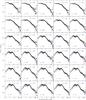 |
Fig. A.1 Overview of the average PSDs at different spectral shapes. PSDs are calculated on a logarithmically binned grid with df/f = 0.15. Each PSD is the average of all n PSDs falling within the Γ1 ± 0.01 interval for the given Γ1 values. Black stars show PSDs in the 2.1–4.5 keV band, red triangles in the 4.5–5.7 keV band, blue circles in the 5.7–9.4 keV, and green squares in the 9.4–15 keV band. The gray line represents the PSD in the total 2.1–15 keV band. |
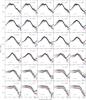 |
Fig. A.2 Overview of the average PSDs at different spectral shapes. PSDs are calculated on a logarithmically binned grid with df/f = 0.15. Each PSD is the average of all n PSDs falling within the Γ1 ± 0.01 interval for the given Γ1 values. Black stars show PSDs in the 2.1–4.5 keV band, red triangles in the 4.5–5.7 keV band, blue circles in the 5.7–9.4 keV, and green squares in the 9.4–15 keV band. The gray line represents the PSD in the total 2.1–15 keV band. The increase in the 2.1–4.5 keV PSDs seen at highest frequencies (especially for Γ1 = 2.61) is not a source-intrinsic effect, but is due to the high flux in this band and resulting telemetry overflow. |
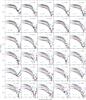 |
Fig. A.3 Overview of the average PSDs at different spectral shapes. PSDs are calculated on a logarithmically binned grid with df/f = 0.15. Each PSD is the average of all n PSDs falling within the Γ1 ± 0.01 interval for the given Γ1 values. Black stars show PSDs in the 2.1–4.5 keV band, red triangles in the 4.5–5.7 keV band, blue circles in the 5.7–9.4 keV, and green squares in the 9.4–15 keV band. The gray line represents the PSD in the total 2.1–15 keV band. The increase in the 2.1–4.5 keV PSDs seen at highest frequencies (especially for Γ1 = 3.25) is not a source intrinsic effect, but is due to the high flux in this band and resulting telemetry overflow. |
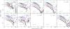 |
Fig. A.4 Overview of the average PSDs at different spectral shapes. PSDs are calculated on a logarithmically binned grid with df/f = 0.15. Each PSD is the average of all n PSDs falling within the Γ1 ± 0.01 interval for the given Γ1 values. Black stars show PSDs in the 2.1–4.5 keV band, red triangles in the 4.5–5.7 keV band, blue circles in the 5.7–9.4 keV, and green squares in the 9.4–15 keV band. The gray line represents the PSD in the total 2.1–15 keV band. |
In our previous study (Grinberg et al. 2013), these seven observations did not receive any special treatment. This does not, however, influence any of our earlier conclusions.
Telemetry overflow is only a problem for the observations with the highest count rate, i.e., the observations at the intermediate to soft state transition (Grinberg et al. 2013). Not all observations at a given Γ1 are, however, affected since spectra with the same Γ1 can vary by a factor of ~4. For example for 2.5 < Γ1< 2.7, the absorbed flux in the 3–10 keV range varies between 4 and 14 keV s-1 cm-2.
Torii et al. (2011) speak only of hard states with high ASM count rates; a comparison with ASM-HID-based state definition of Grinberg et al. (2013) shows that these states are intermediate.
Here and in the rest of this work we use the term “QPO” exclusively for narrow features and do not use the term to describe the broader humps as done, e.g., by Shaposhnikov & Titarchuk (2006). The difference in terminology is phenomenological and does not necessarily imply an assumption of a different origin for the features.
Markowitz et al. (2003) tentatively modeled a second break in the PSD of NGC 3783, but Summons et al. (2007) remeasured the PSD, finding only one break.
Typical frequencies probed in AGN using XMM long looks that allow for lag studies are in the 10-5–10-3 Hz range, corresponding to roughly 10–1000 Hz in black hole binaries. Broadband AGN PSDs are calculated from combined long-term light curves with XMM and RXTE that probe the 10-8–10-3 Hz range, corresponding to roughly 10-2–1000 Hz in black hole binaries.
Acknowledgments
This work has been partially funded by the Bundesministerium für Wirtschaft und Technologie under Deutsches Zentrum für Luft- und Raumfahrt grants 50 OR 1007 and 50 OR 1113 and by the European Commission through ITN 215212 “Black Hole Universe”. It was partially completed by LLNL under contract DE-AC52-07NA27344, and is supported by NASA grants to LLNL and NASA/GSFC. Support for this work was also provided by NASA through the Smithsonian Astrophysical Observatory (SAO) contract SV3-73016 to MIT for Support of the Chandra X-Ray Center (CXC) and Science Instruments; CXC is operated by SAO for and on behalf of NASA under contract NAS8-03060. We further acknowledge support from the DFG Cluster of Excellence “Origin and Structure of the Universe" and are grateful for the support by MCB through the Computational Center for Particle and Astrophysics (C2PAP). This research has made use of NASA’s Astrophysics Data System Bibliographic Services. We thank John E. Davis for the development of the slxfig module used to prepare all figures in this work and Fritz-Walter Schwarm and Ingo Kreykenbohm for their work on the Remeis computing cluster. This research made use of ISIS functions ( isisscripts ) provided by ECAP/Remeis observatory and MIT9. Without the hard work by Evan Smith to schedule the Cyg X-1 so uniformly for more than a decade, this paper would not have been possible. V.G. is grateful for the support through the ESAC faculty grant program to support student attendance at the workshop “Spectral/timing properties of accreting objects: from X-ray binaries to AGN” that proved pivotal for the basic idea behind this research.
References
- Arévalo, P., & Uttley, P. 2006, MNRAS, 367, 801 [NASA ADS] [CrossRef] [Google Scholar]
- Axelsson, M., Borgonovo, L., & Larsson, S. 2005, A&A, 438, 999 [NASA ADS] [CrossRef] [EDP Sciences] [Google Scholar]
- Axelsson, M., Borgonovo, L., & Larsson, S. 2006, A&A, 452, 975 [NASA ADS] [CrossRef] [EDP Sciences] [Google Scholar]
- Belloni, T. M. 2010, in The Jet Paradigm, ed. T. Belloni, (Berlin: Springer), Lect. Notes Phys., 794, 53 [Google Scholar]
- Belloni, T., & Hasinger, G. 1990, A&A, 227, L33 [NASA ADS] [Google Scholar]
- Belloni, T., van der Klis, M., Lewin, W. H. G., et al. 1997, A&A, 322, 857 [NASA ADS] [Google Scholar]
- Belloni, T., Homan, J., Casella, P., et al. 2005, A&A, 440, 207 [NASA ADS] [CrossRef] [EDP Sciences] [Google Scholar]
- Böck, M., Grinberg, V., Pottschmidt, K., et al. 2011, A&A, 533, A8 [NASA ADS] [CrossRef] [EDP Sciences] [Google Scholar]
- Cabanac, C., Roques, J.-P., & Jourdain, E. 2011, ApJ, 739, 58 [NASA ADS] [CrossRef] [Google Scholar]
- Cassatella, P., Uttley, P., & Maccarone, T. J. 2012a, MNRAS, 427, 2985 [NASA ADS] [CrossRef] [Google Scholar]
- Cassatella, P., Uttley, P., Wilms, J., & Poutanen, J. 2012b, MNRAS, 422, 2407 [NASA ADS] [CrossRef] [Google Scholar]
- Churazov, E., Gilfanov, M., & Revnivtsev, M. 2001, MNRAS, 321, 759 [NASA ADS] [CrossRef] [Google Scholar]
- Coppi, P. S. 1999, in High Energy Processes in Accreting Black Holes, eds. J. Poutanen, & R. Svensson, ASP Conf. Ser., 161, 375 [Google Scholar]
- Coppi, P. 2004, in X-ray Timing 2003: Rossi and Beyond, eds. P. Kaaret, F. K. Lamb, & J. H. Swank, AIP Conf. Proc., 714, 79 [Google Scholar]
- Cui, W., Zhang, S. N., Focke, W., & Swank, J. H. 1997, ApJ, 484, 383 [NASA ADS] [CrossRef] [Google Scholar]
- De Marco, B., Ponti, G., Cappi, M., et al. 2013, MNRAS, 431, 2441 [NASA ADS] [CrossRef] [Google Scholar]
- Dhawan, V., Mirabel, I. F., & Rodríguez, L. F. 2000, ApJ, 543, 373 [Google Scholar]
- Done, C., & Gierliński, M. 2005, MNRAS, 364, 208 [NASA ADS] [CrossRef] [Google Scholar]
- Duro, R., Dauser, T., Wilms, J., et al. 2011, A&A, 533, L3 [NASA ADS] [CrossRef] [EDP Sciences] [Google Scholar]
- Fabian, A. C., Zoghbi, A., Ross, R. R., et al. 2009, Nature, 459, 540 [NASA ADS] [CrossRef] [PubMed] [Google Scholar]
- Fender, R. P., Belloni, T. M., & Gallo, E. 2004, MNRAS, 355, 1105 [NASA ADS] [CrossRef] [Google Scholar]
- Fender, R. P., Homan, J., & Belloni, T. M. 2009, MNRAS, 396, 1370 [NASA ADS] [CrossRef] [Google Scholar]
- Fuchs, Y., Rodriguez, J., Mirabel, I. F., et al. 2003, A&A, 409, L35 [NASA ADS] [CrossRef] [EDP Sciences] [Google Scholar]
- Gendreau, K. C., Arzoumanian, Z., & Okajima, T. 2012, in Space Telescopes and Instrumentation 2012: Ultraviolet to Gamma Ray, Proc. SPIE, 8443, 844313 [Google Scholar]
- Giannios, D., Kylafis, N. D., & Psaltis, D. 2004, A&A, 425, 163 [NASA ADS] [CrossRef] [EDP Sciences] [Google Scholar]
- Gierliński, M., & Zdziarski, A. A. 2005, MNRAS, 363, 1349 [NASA ADS] [CrossRef] [Google Scholar]
- Gierliński, M., Nikołajuk, M., & Czerny, B. 2008, MNRAS, 383, 741 [NASA ADS] [CrossRef] [Google Scholar]
- Gierliński, M., Zdziarski, A. A., & Done, C. 2010, in Frontier Objects in Astrophysics and Particle Physics, eds. F. Giovannelli, & G. Mannocchi, Italian Phys. Soc. Conf. Proc. 203, 299 [Google Scholar]
- Gilfanov, M., Churazov, E., & Revnivtsev, M. 1999, A&A, 352, 182 [NASA ADS] [Google Scholar]
- Gleissner, T., Wilms, J., Pooley, G. G., et al. 2004a, A&A, 425, 1061 [NASA ADS] [CrossRef] [EDP Sciences] [Google Scholar]
- Gleissner, T., Wilms, J., Pottschmidt, K., et al. 2004b, A&A, 414, 1091 [NASA ADS] [CrossRef] [EDP Sciences] [Google Scholar]
- González-Martín, O., & Vaughan, S. 2012, A&A, 544, A80 [NASA ADS] [CrossRef] [EDP Sciences] [Google Scholar]
- Grinberg, V., Hell, N., Pottschmidt, K., et al. 2013, A&A, 554, A88 [NASA ADS] [CrossRef] [EDP Sciences] [Google Scholar]
- Hanke, M. 2011, Ph.D. Thesis, Dissertation, Universität Erlangen-Nürnberg, Germany [Google Scholar]
- Homan, J., Wijnands, R., van der Klis, M., et al. 2001, ApJS, 132, 377 [NASA ADS] [CrossRef] [Google Scholar]
- Houck, J. C. 2002, in High Resolution X-ray Spectroscopy with XMM-Newton and Chandra, Proc. international workshop held at Mullard Space Science Laboratory of University College London, ed. G. Branduardi-Raymont, published electronically [Google Scholar]
- Houck, J. C., & Denicola, L. A. 2000, in Astronomical Data Analysis Software and Systems IX, eds. N. Manset, C. Veillet, & D. Crabtree, ASP Conf. Ser., 216, 591 [Google Scholar]
- Ingram, A., & Done, C. 2011, MNRAS, 415, 2323 [NASA ADS] [CrossRef] [Google Scholar]
- Ingram, A., & Done, C. 2012, MNRAS, 419, 2369 [NASA ADS] [CrossRef] [Google Scholar]
- Ingram, A., & van der Klis, M. 2013, MNRAS, 434, 1476 [NASA ADS] [CrossRef] [Google Scholar]
- Jahoda, K., Markwardt, C. B., Radeva, Y., et al. 2006, ApJS, 163, 401 [NASA ADS] [CrossRef] [Google Scholar]
- Jourdain, E., Roques, J. P., Chauvin, M., & Clark, D. J. 2012, ApJ, 761, 27 [NASA ADS] [CrossRef] [Google Scholar]
- Kalemci, E., Tomsick, J. A., Rothschild, R. E., et al. 2003, ApJ, 586, 419 [NASA ADS] [CrossRef] [Google Scholar]
- Kalemci, E., Tomsick, J. A., Rothschild, R. E., Pottschmidt, K., & Kaaret, P. 2004, ApJ, 603, 231 [Google Scholar]
- Klein, R. W., & Roberts, S. D. 1984, SIMULATION, 43, 193 [Google Scholar]
- Klein-Wolt, M., & van der Klis, M. 2008, ApJ, 675, 1407 [NASA ADS] [CrossRef] [Google Scholar]
- Körding, E., & Falcke, H. 2004, A&A, 414, 795 [NASA ADS] [CrossRef] [EDP Sciences] [Google Scholar]
- Körding, E. G., Jester, S., & Fender, R. 2006, MNRAS, 372, 1366 [NASA ADS] [CrossRef] [Google Scholar]
- Körding, E., Rupen, M., Knigge, C., et al. 2008, Science, 320, 1318 [NASA ADS] [CrossRef] [PubMed] [Google Scholar]
- Kotov, O., Churazov, E., & Gilfanov, M. 2001, MNRAS, 327, 799 [NASA ADS] [CrossRef] [Google Scholar]
- Kylafis, N. D., Papadakis, I. E., Reig, P., Giannios, D., & Pooley, G. G. 2008, A&A, 489, 481 [NASA ADS] [CrossRef] [EDP Sciences] [Google Scholar]
- Laurent, P., Rodriguez, J., Wilms, J., et al. 2011, Science, 332, 438 [NASA ADS] [CrossRef] [PubMed] [Google Scholar]
- Levine, A. M., Bradt, H., Cui, W., et al. 1996, ApJ, 469, L33 [NASA ADS] [CrossRef] [Google Scholar]
- Lightman, A. P., & Eardley, D. M. 1974, ApJ, 187, L1 [NASA ADS] [CrossRef] [Google Scholar]
- Lyubarskii, Y. E. 1997, MNRAS, 292, 679 [NASA ADS] [CrossRef] [Google Scholar]
- Maitra, D., & Bailyn, C. D. 2004, ApJ, 608, 444 [NASA ADS] [CrossRef] [Google Scholar]
- Maitra, D., Markoff, S., Brocksopp, C., et al. 2009, MNRAS, 398, 1638 [NASA ADS] [CrossRef] [Google Scholar]
- Makishima, K., Maejima, Y., Mitsuda, K., et al. 1986, ApJ, 308, 635 [NASA ADS] [CrossRef] [Google Scholar]
- Manmoto, T., Takeuchi, M., Mineshige, S., Matsumoto, R., & Negoro, H. 1996, ApJ, 464, L135 [NASA ADS] [CrossRef] [Google Scholar]
- Markoff, S., Nowak, M. A., & Wilms, J. 2005, ApJ, 635, 1203 [NASA ADS] [CrossRef] [Google Scholar]
- Markowitz, A. 2005, ApJ, 635, 180 [NASA ADS] [CrossRef] [Google Scholar]
- Markowitz, A. 2010, ApJ, 724, 26 [NASA ADS] [CrossRef] [Google Scholar]
- Markowitz, A., Edelson, R., Vaughan, S., et al. 2003, ApJ, 593, 96 [NASA ADS] [CrossRef] [Google Scholar]
- Markowitz, A., Papadakis, I., Arévalo, P., et al. 2007, ApJ, 656, 116 [NASA ADS] [CrossRef] [Google Scholar]
- McClintock, J. E., & Remillard, R. A. 2006, in Compact Stellar X-ray Sources, eds. W. Lewin, & M. van der Klis (Cambridge: Cambridge Univ. Press), 157 [Google Scholar]
- McHardy, I. M. 2010, in The Jet Paradigm, ed. T. Belloni (Berlin: Springer), Lect. Notes Phys., 794, 203 [Google Scholar]
- McHardy, I. M., Papadakis, I. E., Uttley, P., Page, M. J., & Mason, K. O. 2004, MNRAS, 348, 783 [NASA ADS] [CrossRef] [Google Scholar]
- McHardy, I. M., Körding, E., Knigge, C., Uttley, P., & Fender, R. P. 2006, Nature, 444, 730 [NASA ADS] [CrossRef] [PubMed] [Google Scholar]
- McHardy, I. M., Arévalo, P., Uttley, P., et al. 2007, MNRAS, 382, 985 [NASA ADS] [CrossRef] [Google Scholar]
- McKinney, J. C., Tchekhovskoy, A., & Blandford, R. D. 2012, MNRAS, 423, 3083 [NASA ADS] [CrossRef] [Google Scholar]
- Mitsuda, K., Inoue, H., Koyama, K., et al. 1984, PASJ, 36, 741 [NASA ADS] [Google Scholar]
- Miyamoto, S., & Kitamoto, S. 1989, Nature, 342, 773 [NASA ADS] [CrossRef] [Google Scholar]
- Miyamoto, S., Kitamoto, S., Mitsuda, K., & Dotani, T. 1988, Nature, 336, 450 [NASA ADS] [CrossRef] [Google Scholar]
- Miyamoto, S., Kimura, K., Kitamoto, S., Dotani, T., & Ebisawa, K. 1991, ApJ, 383, 784 [NASA ADS] [CrossRef] [Google Scholar]
- Muñoz-Darias, T., Motta, S., Pawar, D., et al. 2010, MNRAS, 404, L94 [NASA ADS] [CrossRef] [Google Scholar]
- Muñoz-Darias, T., Motta, S., Stiele, H., & Belloni, T. M. 2011, MNRAS, 415, 292 [NASA ADS] [CrossRef] [Google Scholar]
- Nandra, K., & Papadakis, I. E. 2001, ApJ, 554, 710 [NASA ADS] [CrossRef] [Google Scholar]
- Noble, M. S., & Nowak, M. A. 2008, PASP, 120, 821 [NASA ADS] [CrossRef] [Google Scholar]
- Nowak, M. A. 1995, PASP, 107, 1207 [NASA ADS] [CrossRef] [Google Scholar]
- Nowak, M. A. 2000, MNRAS, 318, 361 [NASA ADS] [CrossRef] [Google Scholar]
- Nowak, M. A., Vaughan, B. A., Wilms, J., Dove, J. B., & Begelman, M. C. 1999a, ApJ, 510, 874 [NASA ADS] [CrossRef] [Google Scholar]
- Nowak, M. A., Wilms, J., Vaughan, B. A., Dove, J. B., & Begelman, M. C. 1999b, ApJ, 515, 726 [NASA ADS] [CrossRef] [Google Scholar]
- Nowak, M. A., Hanke, M., Trowbridge, S. N., et al. 2011, ApJ, 728, 13 [NASA ADS] [CrossRef] [Google Scholar]
- Nowak, M. A., Wilms, J., Hanke, M., Pottschmidt, K., & Markoff, S. 2012, Mem. Soc. Astron. It., 83, 202 [NASA ADS] [Google Scholar]
- Orosz, J. A., McClintock, J. E., Aufdenberg, J. P., et al. 2011, ApJ, 742, 84 [NASA ADS] [CrossRef] [Google Scholar]
- Papadakis, I. E., Sobolewska, M., Arévalo, P., et al. 2009, A&A, 494, 905 [NASA ADS] [CrossRef] [EDP Sciences] [Google Scholar]
- Paul, B. 2013, Int. J. Mod. Phys. D, 22, 1341009 [NASA ADS] [CrossRef] [Google Scholar]
- Pottschmidt, K. 2002, Ph.D. Thesis, Dissertation, Universität Tübingen, Germany [Google Scholar]
- Pottschmidt, K., Wilms, J., Nowak, M. A., et al. 2000, A&A, 357, L17 [NASA ADS] [Google Scholar]
- Pottschmidt, K., Wilms, J., Nowak, M. A., et al. 2003, A&A, 407, 1039 [NASA ADS] [CrossRef] [EDP Sciences] [Google Scholar]
- Pottschmidt, K., Wilms, J., Nowak, M. A., et al. 2006, Adv. Space Res., 38, 1350 [NASA ADS] [CrossRef] [Google Scholar]
- Psaltis, D., & Norman, C. 2000, unpublished [arXiv:astro-ph/0001391] [Google Scholar]
- Reid, M. J., McClintock, J. E., Narayan, R., et al. 2011, ApJ, 742, 83 [NASA ADS] [CrossRef] [Google Scholar]
- Reig, P., Kylafis, N. D., & Giannios, D. 2003, A&A, 403, L15 [NASA ADS] [CrossRef] [EDP Sciences] [Google Scholar]
- Revnivtsev, M., Gilfanov, M., & Churazov, E. 2000, A&A, 363, 1013 [NASA ADS] [Google Scholar]
- Reynolds, C. S., & Nowak, M. A. 2003, Phys. Rep., 377, 389 [NASA ADS] [CrossRef] [Google Scholar]
- Rodriguez, J., Varnière, P., Tagger, M., & Durouchoux, P. 2002, A&A, 387, 487 [NASA ADS] [CrossRef] [EDP Sciences] [Google Scholar]
- Rodriguez, J., Corbel, S., Kalemci, E., Tomsick, J. A., & Tagger, M. 2004, ApJ, 612, 1018 [NASA ADS] [CrossRef] [Google Scholar]
- Rothschild, R. E., Blanco, P. R., Gruber, D. E., et al. 1998, ApJ, 496, 538 [NASA ADS] [CrossRef] [Google Scholar]
- Scaringi, S., Körding, E., Groot, P. J., et al. 2013, MNRAS, 431, 2535 [NASA ADS] [CrossRef] [Google Scholar]
- Schmid, C. 2012, Ph.D. Thesis, Dissertation, Universität Erlangen-Nürnberg, Germany [Google Scholar]
- Schnittman, J. D., Krolik, J. H., & Noble, S. C. 2013, ApJ, 769, 156 [NASA ADS] [CrossRef] [Google Scholar]
- Shakura, N. I., & Sunyaev, R. A. 1976, MNRAS, 175, 613 [NASA ADS] [CrossRef] [Google Scholar]
- Shaposhnikov, N., & Titarchuk, L. 2006, ApJ, 643, 1098 [NASA ADS] [CrossRef] [Google Scholar]
- Skipper, C. J., McHardy, I. M., & Maccarone, T. J. 2013, MNRAS, 434, 574 [NASA ADS] [CrossRef] [Google Scholar]
- Soleri, P., Muñoz-Darias, T., Motta, S., et al. 2013, MNRAS, 429, 1244 [NASA ADS] [CrossRef] [Google Scholar]
- Sriram, K., Agrawal, V. K., & Rao, A. R. 2009, ApJ, 700, 1042 [NASA ADS] [CrossRef] [Google Scholar]
- Stiele, H., Belloni, T. M., Kalemci, E., & Motta, S. 2013, MNRAS, 429, 2655 [NASA ADS] [CrossRef] [Google Scholar]
- Stirling, A. M., Spencer, R. E., de la Force, C. J., et al. 2001, MNRAS, 327, 1273 [NASA ADS] [CrossRef] [Google Scholar]
- Summons, D. P., Arévalo, P., McHardy, I. M., Uttley, P., & Bhaskar, A. 2007, MNRAS, 378, 649 [NASA ADS] [CrossRef] [Google Scholar]
- Tagger, M., & Pellat, R. 1999, A&A, 349, 1003 [NASA ADS] [Google Scholar]
- Timmer, J., & König, M. 1995, A&A, 300, 707 [NASA ADS] [Google Scholar]
- Tomsick, J. A., Nowak, M. A., Parker, M., et al. 2014, ApJ, 780, 78 [NASA ADS] [CrossRef] [Google Scholar]
- Torii, S., Yamada, S., Makishima, K., et al. 2011, PASJ, 63, 771 [Google Scholar]
- Uttley, P., Wilkinson, T., Cassatella, P., et al. 2011, MNRAS, 414, L60 [NASA ADS] [Google Scholar]
- Varnière, P., Tagger, M., & Rodriguez, J. 2011, A&A, 525, A87 [NASA ADS] [CrossRef] [EDP Sciences] [Google Scholar]
- Varnière, P., Tagger, M., & Rodriguez, J. 2012, A&A, 545, A40 [NASA ADS] [CrossRef] [EDP Sciences] [Google Scholar]
- Vaughan, B. A., & Nowak, M. A. 1997, ApJ, 474, L43 [NASA ADS] [CrossRef] [Google Scholar]
- Vaughan, S., Fabian, A. C., & Nandra, K. 2003, MNRAS, 339, 1237 [NASA ADS] [CrossRef] [Google Scholar]
- Verner, D. A., Ferland, G. J., Korista, K. T., & Yakovlev, D. G. 1996, ApJ, 465, 487 [NASA ADS] [CrossRef] [Google Scholar]
- Vrtilek, S. D., & Boroson, B. S. 2013, MNRAS, 428, 3693 [NASA ADS] [CrossRef] [Google Scholar]
- Wilkinson, T., & Uttley, P. 2009, MNRAS, 397, 666 [NASA ADS] [CrossRef] [Google Scholar]
- Wilms, J., Allen, A., & McCray, R. 2000, ApJ, 542, 914 [NASA ADS] [CrossRef] [Google Scholar]
- Wilms, J., Nowak, M. A., Pottschmidt, K., Pooley, G. G., & Fritz, S. 2006, A&A, 447, 245 [NASA ADS] [CrossRef] [EDP Sciences] [Google Scholar]
- Xiang, J., Lee, J. C., Nowak, M. A., & Wilms, J. 2011, ApJ, 738, 78 [NASA ADS] [CrossRef] [Google Scholar]
All Tables
All Figures
|
Fig. 1 Evolution of Cyg X-1 over the RXTE lifetime. Vertical lines represent the starting times of the RXTE calibration epochs used in this work: dashed line for epoch 3, dot-dashed line for epoch 4, and dot-dot-dashed line for epoch 5. The total ASM count rate is color-coded according to ASM-based state definition of Grinberg et al. (2013), which uses both ASM count rate and ASM hardness of a given measurement: blue represents the hard state, green the intermediate state, and red the soft state. ASM data points after MJD 55 200 are affected by instrumental decline (Vrtilek & Boroson 2013; Grinberg et al. 2013) and shown in gray. The soft photon index Γ1 is shown only for those 1980 RXTE observations that were conducted in the B_2ms_8B_0_35_Q binned data mode, see Sect. 2.3. The rms is calculated in the 0.125–256 Hz range (Sect. 3.1), the time lags are averaged values in the 3.2–10 Hz range (Sect. 4.3). |
| In the text | |
|
Fig. 2 Number of orbit-wise RXTE observations of Cyg X-1 in the B_2ms_8B_0_35_Q mode with a given Γ1. Shown are both observations that require a disk (red) and do not require a disk (blue), and the total number of observations (gray). |
| In the text | |
|
Fig. 3 Fractional rms in the 2.1–15 keV band vs. soft photon index Γ1. |
| In the text | |
|
Fig. 4 Fractional rms in the 0.125–256 Hz frequency band for different energy bands vs. the soft photon index, Γ1, of the broken power law fits. |
| In the text | |
|
Fig. 5 Ratio of fractional rms in different energy bands (band 1 – rms1, band 2 – rms2, band 4 – rms4,) vs. soft photon index Γ1. |
| In the text | |
|
Fig. 6 Evolution of fractional rms between 0.125–256 Hz in the eight binned channels of the B_2ms_8B_0_35_Q mode with the X-ray spectral shape represented by the soft photon index Γ1. Black horizontal lines are photon indices for which no data are available. |
| In the text | |
|
Fig. 7 Evolution of PSDs in 2.1–15 keV band (sum of bands 1–4 and full energy range of the B_2ms_8B_0_35_Q mode) with spectral shape. The color scale represents averaged PSD(fi) × fi values at individual Fourier frequencies fi. In this and in all following figures, black vertical lines are photon indices for which no data are available. |
| In the text | |
|
Fig. 8 Evolution of the PSDs with spectral shape represented by the soft photon index Γ1 of the broken power law fit in four energy bands (see Table 1). The color scale represents averaged PSD(fi) × fi values at individual Fourier frequencies fi. |
| In the text | |
|
Fig. 9 Comparison of average PSDs for Γ1 ~ 1.67 (blue stars) and Γ1 ~ 3.49 (red squares). PSDs are calculated for a logarithmically binned grid with df/f = 0.15. Each PSD is the average of all n PSDs falling within the Γ1 ± 0.01 interval for the given Γ1 values. Left: band 2 (5.7–9.4 keV). Right: total band (2.1–15 keV). |
| In the text | |
|
Fig. 10 Evolution of the coherence, γ2, with spectral shape represented by the soft photon index Γ1 of the broken power law. The color scale represents averaged γ2 values at individual Fourier frequencies fi. Upper panel: |
| In the text | |
|
Fig. 11 Evolution of time lags δt in the |
| In the text | |
|
Fig. 12 Averaged time lag in the 3.2–10 Hz range vs. soft photon index of the broken power law fits Γ1 for all combinations of energy bands (band 1: 2.1–4.5 keV, band 2: 4.5–5.7 keV, band 3: 5.7–9.4 keV, band 4: 9.4–15 keV). Zero time lag is represented by the dashed red line. |
| In the text | |
|
Fig. A.1 Overview of the average PSDs at different spectral shapes. PSDs are calculated on a logarithmically binned grid with df/f = 0.15. Each PSD is the average of all n PSDs falling within the Γ1 ± 0.01 interval for the given Γ1 values. Black stars show PSDs in the 2.1–4.5 keV band, red triangles in the 4.5–5.7 keV band, blue circles in the 5.7–9.4 keV, and green squares in the 9.4–15 keV band. The gray line represents the PSD in the total 2.1–15 keV band. |
| In the text | |
|
Fig. A.2 Overview of the average PSDs at different spectral shapes. PSDs are calculated on a logarithmically binned grid with df/f = 0.15. Each PSD is the average of all n PSDs falling within the Γ1 ± 0.01 interval for the given Γ1 values. Black stars show PSDs in the 2.1–4.5 keV band, red triangles in the 4.5–5.7 keV band, blue circles in the 5.7–9.4 keV, and green squares in the 9.4–15 keV band. The gray line represents the PSD in the total 2.1–15 keV band. The increase in the 2.1–4.5 keV PSDs seen at highest frequencies (especially for Γ1 = 2.61) is not a source-intrinsic effect, but is due to the high flux in this band and resulting telemetry overflow. |
| In the text | |
|
Fig. A.3 Overview of the average PSDs at different spectral shapes. PSDs are calculated on a logarithmically binned grid with df/f = 0.15. Each PSD is the average of all n PSDs falling within the Γ1 ± 0.01 interval for the given Γ1 values. Black stars show PSDs in the 2.1–4.5 keV band, red triangles in the 4.5–5.7 keV band, blue circles in the 5.7–9.4 keV, and green squares in the 9.4–15 keV band. The gray line represents the PSD in the total 2.1–15 keV band. The increase in the 2.1–4.5 keV PSDs seen at highest frequencies (especially for Γ1 = 3.25) is not a source intrinsic effect, but is due to the high flux in this band and resulting telemetry overflow. |
| In the text | |
|
Fig. A.4 Overview of the average PSDs at different spectral shapes. PSDs are calculated on a logarithmically binned grid with df/f = 0.15. Each PSD is the average of all n PSDs falling within the Γ1 ± 0.01 interval for the given Γ1 values. Black stars show PSDs in the 2.1–4.5 keV band, red triangles in the 4.5–5.7 keV band, blue circles in the 5.7–9.4 keV, and green squares in the 9.4–15 keV band. The gray line represents the PSD in the total 2.1–15 keV band. |
| In the text | |
Current usage metrics show cumulative count of Article Views (full-text article views including HTML views, PDF and ePub downloads, according to the available data) and Abstracts Views on Vision4Press platform.
Data correspond to usage on the plateform after 2015. The current usage metrics is available 48-96 hours after online publication and is updated daily on week days.
Initial download of the metrics may take a while.