| Issue |
A&A
Volume 565, May 2014
|
|
|---|---|---|
| Article Number | A7 | |
| Number of page(s) | 9 | |
| Section | Planets and planetary systems | |
| DOI | https://doi.org/10.1051/0004-6361/201321087 | |
| Published online | 18 April 2014 | |
Ground-based transit observations of the super-Earth GJ 1214 b⋆,⋆⋆
1
Instituto de Física y Astronomía, Universidad de
Valparaíso, Av. Gran Bretaña 1111,
2360102
Valparaíso,
Chile
e-mail:
This email address is being protected from spambots. You need JavaScript enabled to view it.
2
Millenium Nucleus “Protoplanetary Disks in ALMA Early Science”,
Universidad de Valparaíso, 2360102
Valparaíso,
Chile
3
European Southern Observatory, Av. Alonso de Córdova 3107, Vitacura, 19001
Santiago,
Chile
4
Instituto de Astrofísica de Canarias, Vía Láctea s/n, 38200 – La Laguna, Tenerife,
Canary Islands,
Spain
5
Department of Astrophysics, University of La Laguna,
Vía Láctea s/n, 38200-La Laguna,
Tenerife, Canary
Islands, Spain
6
Universidad de Chile, Camino El Observatorio 1515,
Las Condes, Casilla
36- D Santiago,
Chile
7
Department of Physics, Grinnell College, Grinnell, IA
50112,
USA
8
University of California, Santa Cruz, Department of Astronomy
& Astrophysics, 1156
High Street, Santa
Cruz, CA
95064,
USA
9
Pontificia Universidad Católica de Chile, Departamento de
Astronomía y Astrofísica, Av.
Vicuña Mackenna 4860, 782-0436 Macul, Santiago, Chile
10
Specola Vaticana, 00120
Vatican City State,
Italy
Received: 11 January 2013
Accepted: 5 March 2014
Abstract
Context. GJ 1214 b is one of the few known transiting super-Earth-sized exoplanets with a measured mass and radius. It orbits an M-dwarf, only 14.55 pc away, making it a favorable candidate for follow-up studies. However, the composition of GJ 1214 b’s mysterious atmosphere has yet to be fully unveiled.
Aims. Our goal is to distinguish between the various proposed atmospheric models to explain the properties of GJ 1214 b: hydrogen-rich or hydrogen-He mix, or a heavy molecular weight atmosphere with reflecting high clouds, as latest studies have suggested.
Methods. Wavelength-dependent planetary radii measurements from the transit depths in the optical/NIR are the best tool to investigate the atmosphere of GJ 1214 b. We present here (i) photometric transit observations with a narrow-band filter centered on 2.14 μm and a broad-band I-Bessel filter centered on 0.8665 μm, and (ii) transmission spectroscopy in the H and K atmospheric windows that cover three transits. The photometric and spectrophotometric time series obtained were analyzed with MCMC simulations to measure the planetary radii as a function of wavelength. We determined radii ratios of 0.1173-0.0024+0.0022 for I-Bessel and 0.11735-0.00076+0.00072 at 2.14 μm.
Results. Our measurements indicate a flat transmission spectrum, in agreement with the last atmospheric models that favor featureless spectra with clouds and high molecular weight compositions.
Key words: planetary systems / techniques: photometric / techniques: spectroscopic / planets and satellites: atmospheres / stars: individual: GJ 1214
Based on observations obtained at the Southern Astrophysical Research (SOAR) Telescope, which is a joint project of the Ministério da Ciência, Tecnologia, e Inovação (MCTI) da República Federativa do Brasil, the US National Optical Astronomy Observatory (NOAO), the University of North Carolina at Chapel Hill (UNC), and Michigan State University (MSU). SofI results are based on observations made with ESO Telescopes at the La Silla Paranal Observatory under programme ID 087.C-0509.
Tables of the lightcurve data are only available at the CDS via anonymous ftp to cdsarc.u-strasbg.fr (130.79.128.5) or via http://cdsarc.u-strasbg.fr/viz-bin/qcat?J/A+A/565/A7
© ESO, 2014
1. Introduction
The handful of known transiting extrasolar super-Earths have been mostly found by space missions such as Kepler, CoRoT, or MOST, with the notable exception of GJ 1214 b (2.7 R⊕, 6.55 M⊕), which was discovered by the ground-based transiting survey MEarth around a bright nearby M-star (Charbonneau et al. 2009). Despite the relatively small radius of GJ 1214 b, the small stellar radius of its host star results in a ~1.5% transit depth, making it one of the super-Earths best suited for follow-up studies.
The recent theoretical predictions for the atmosphere of GJ 1214 b currently offer the most plausible models that fit the planet’s mass, radius, and irradiation level: a rocky or an icy core with a nebular hydrogen-helium envelope, that is, a mini-Neptune, a rocky planet with an outgassed hydrogen atmosphere, or a core with a heavy (up to 45% of the planet mass) hot water vapor envelope with high molecular mass (Rogers & Seager 2010; Nettelmann et al. 2011), as well as a planet with a cloudy or hazy atmosphere, with a high mean molecular mass composition (Morley et al. 2013).
GJ 1214 b has been the target of an intensive observing campaign. Bean et al. (2010) reported a flat optical transmission spectrum that ruled out a cloud-free mini-Neptune model. This conclusion was supported by additional transit observations of Bean et al. (2011), Berta et al. (2012), and Crossfield et al. (2011) in the near-infrared (NIR) region, and Désert et al. (2011) in the mid-infrared. However, Croll et al. (2011) measured a deeper 2.2 μm transit, implying H2 absorption, consistent with a mini-Neptune model. Transient achromatic haze might reconcile these observations, but the close dates of the K-band observations of Croll et al. (2011) and Crossfield et al. (2011) make it unlikely, and as Berta et al. (2012) pointed out, there is no known source of achromatic haze. Strangely, Narita et al. (2013b) reported J- and H-band observations consistent with a flat featureless transmission spectrum, but shallower KS-band transmission depth, in disagreement with the result of Croll et al. (2011). Fraine et al. (2012) also reported constant planetary atmosphere radii at I + z, 3.6 μm, and 4.5 μm. Finally, Murgas et al. (2012) found a radius of GJ 1214 b at the Hα line higher than the radii measured at nearby continua, but the difference is not statistically significant. The latest observations reported by Teske et al. (2013), Colón & Gaidos (2013), Wilson et al. (2014), Gillon et al. (2014), de Mooij et al. (2013), and Kreidberg et al. (2014) have agreed in showing a featureless spectrum, favoring high mean molecular mass compositions. In that context, recently Kreidberg et al. (2014) ruled out the cloud-free high molecular weight atmosphere scenario for GJ 1214b with a high statistical significance.
Here we report new optical and NIR ground-based observations of GJ 1214 b transits, aiming to independently verify these results. The paper is organized as follows: Sect. 2 presents our observations, Sect. 3 describes the analysis, Sect. 4 presents a discussion of our results, and Sect. 5 is a summary of the main points of this paper.
2. Observations and data reduction
2.1. NIR photometry with OSIRIS
We observed a GJ 1214 b transit from UT 0:19 to 4:10 on the night of 09 August 2011 with the Ohio State Infrared Imager/Spectrometer (OSIRIS; Depoy et al. 1993) at the 4.1 m Southern Astrophysical Research (SOAR) Telescope at Cerro Pachón, Chile. OSIRIS only uses a 577 × 577 px window from a 1024 × 1024 px HgCdTe array, yielding 191 × 191 arcsec field of view (FoV) (pixel scale 0.331 arcsec px-1). A narrow-band (1%) filter centered on 2.14 μm was used. We placed GJ 1214 and a nearby reference star (2MASS J17152424+0455041) within the FOV. They have similar apparent brightness and are separated by ~3 arcmin.
The observations were carried out in stare mode, that is, the stars were kept on the same positions to minimize the systematic effects associated with inaccurate flat-fielding and intra-pixel sensitivity variations. A total of 1,030 science images were collected, with exposure times ranging from 5 to 20 s, which had to be adjusted to avoid reaching the nonlinearity regime under variable seeing and airmass.
First, we subtracted the dark current by scaling one series of darks to match the different exposure times used throughout the night, and flat-fielded the images. To extract the apparent fluxes from the reduced images we carried out aperture photometry with the IRAF Digiphot package1. Led by our previous experience with stare-mode NIR data, we removed the sky by measuring it in circular annuli, contiguous to the aperture centered on the object (Cáceres et al. 2009, 2011). We performed photometry for different aperture radii, ranging from 4.0 to 14.0 px, in steps of 0.5 px, and selected the combination of source and sky apertures that minimizes the root mean square (rms) of the final differential light curve: target and reference aperture radii of 2.32 arcsec, and a sky annulus with 4.9 arcsec inner radius and 3.3 arcsec width. The generated light curve is shown in Fig. 1 (top).
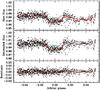 |
Fig. 1 2.14 μm GJ 1214 b photometric series obtained with OSIRIS. Top: raw light curve, with the best-fitting transit model in red. Middle: de-trended light curve with the best-fitting model. Bottom: residuals from the best-fitting model; the rms. is 0.0062. This figure is available in color in electronic form. |
Observing log for the spectroscopic SofI Observations of GJ 1214 b.
2.2. Optical photometry with SOI
A transit of GJ 1214 b was observed in the I-Bessel filter from UT 04:03 to 09:30 on the night of April 28, 2010 with the SOAR Optical Imager (SOI) at the SOAR telescope on Cerro Pachón. The instrument has a mosaic of two E2V 2 × 4 k CCDs, covering a ~5.5 × 5.5 arcmin FoV (pixel scale 0.077 arcsec px-1). The binning was 2 × 2, and the readout time was 11 s.
We placed the target close to the center of the FoV, which allowed us to observe eight reference stars of similar or slightly fainter brightness to that of the target. We obtained 1730 frames, with integration times between 3 and 5 s – adjusted throughout the night to keep the core of the stellar images in the linear regimen.
The basic data reduction included trimming the images, bias subtraction and flat-fielding corrections with SOI’s custom-made pipeline (Hoyer et al. 2012). Next, we performed standard aperture photometry of the target and the eight reference stars. The optimal aperture and sky-annulus radii were selected to minimize the rms of the portions of the light curve before and after the transit, best values being stellar aperture radius – 18 pix, sky annulus radius – 20 pix and 10 pix in width. Similarly, our experiments with the reference stars demonstrated that the best light curve is obtained using only one of them – the brightest 2MASS J17152424+0455041 (KS = 8.983 mag). According to our tests, adding more reference stars increased the noise. The generated light curve is shown in Fig. 2 (top).
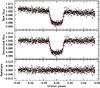 |
Fig. 2 I-Bessel GJ 1214 b photometric series obtained with SOI. Top: raw light curve, with the best-fitting transit model in red. Middle: de-trended light curve with the best-fitting model. Bottom: residuals from the best-fitting model; the rms is 0.0019. This figure is available in color in electronic form. |
2.3. NIR spectrophotometry with SofI
Three GJ 1214 b transits were observed with the NIR spectrograph SofI (Son of ISAAC; Moorwood et al. 1998) at the ESO New Technology Telescope (see Table 1). The instrument is equipped with a 1024 × 1024 Hawaii detector and ~4.9 arcmin long slits (pixel scale 0.292 arcsec px-1). The red grism was used, providing a spectral coverage from λ ~ 1.5 to 2.5 μm.
A comparison star (2MASS J17152424+0455041; ~3.06 arcmin separation from the target) of similar spectral type and brightness as GJ 1214 was placed in the slit at all times for continuous and simultaneous monitoring of the telluric absorption. The observations were performed in stare mode, that is, without nodding, to keep the objects on nearly the same pixels, minimizing effects from flat-fielding errors and intra-pixel sensitivity variations. The NDIT × DIT combination was chosen to keep the peak count level at ~6000 ADU, well below the ~1.5% nonlinearity limit of 10 000 ADU.
The first steps of the basic data reduction were the usual cross-talk and flat-fielding corrections, and bad-pixel replacement. However, the stare mode made it impossible to remove the sky emission by subtracting corresponding nodding image pairs, as is normally done. Instead, we took advantage of having small field distortions and bright targets to individually trace their continuum on each frame, and to extract at each side of the objects two adjacent sky emission spectra. Then, we subtracted from each object’s one-dimensional spectrum the linearly interpolated value of the two one-dimensional sky spectra that correspond to the location of the object. Since the sky spectra also include the dark and bias contributions, we successfully removed the detector pattern from our data as well. These steps were performed with the task apall from the IRAF package twodspec.
The wavelength calibration is based on xenon lamp spectra-for each object and each frame we separately extracted a one-dimensional lamp spectrum from the lamp frame using the same tracing and extraction aperture as for that object on that frame. Typically, nine Xe lines were used in the calibration, and the rms was 1–2 Å. A typical target spectrum at this stage of the processing is shown in Fig. 3.
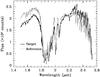 |
Fig. 3 Typical wavelength-calibrated one-dimensional spectrum of GJ 1214 b, not corrected for telluric absorption, obtained with SofI on May 17/18, 2011. |
The telluric absorption was removed by dividing in the wavelength space the planet’s host spectrum by the spectrum of the reference star. This was done separately for each individual frame, ensuring that the absorption variations are accounted for, because the two spectra were obtained simultaneously and very close on the sky.
Finally, we integrated the flux in the reduced spectra within selected bandpasses – the standard SofI NIR broad-band filters, H (λC = 1.653 μm, FWHM = 0.297 μm) and KS (λC = 2.162 μm, FWHM = 0.275 μm). We refrained from splitting the data into finer spectral bins because of the low signal-to-noise ratio of the data. The individual spectrophotometric series for GJ 1214 b and its comparison star are shown in Fig. 4, and the composed light curves are shown in Fig. 5 (top).
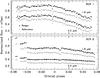 |
Fig. 4 Spectrophotometric individual time series obtained from integrating the flux of the SofI spectra within the H and KS bands for the target and its comparison stars, and for the two good-weather runs. |
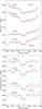 |
Fig. 5 H (1.6 μm) and KS (2.2 μm) GJ 1214 b spectrophotometric series obtained from integrating the flux of the SofI spectra within the H and KS bands. Top: raw light curves, with the best-fitting transit models in red. Bottom: de-trended light curves with the best-fitting models. This figure is available in color in electronic form. |
3. Data analysis
3.1. OSIRIS and SOI data
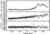 |
Fig. 6 Parameters used to de-trend the OSIRIS photometric time series. From top to bottom: sky flux value and (ΔxC,ΔyC), the variations of the target’s position coordinates around their median value. |
Despite the intrinsic correction of systematics due to differential nature of the photometry, the OSIRIS raw light curve of GJ 1214 b shows significant structure, especially in the second half of the observations (Fig. 1, top). We found strong correlations of the out-of-transit flux measurements with both the (xC,yC) position of the stellar centroids on the detector, and the sky flux level ms – related to guiding errors, residual flat-field errors, and to variable weather conditions (Fig. 6).
To extract the physical parameters from the obtained light curves we fit the photometric time series with both a transit model Θ(t), and a linear model κ(t) that accounts for the systematics observed in the light curve. The best combination of parameters we found to de-trend the OSIRIS light curve was  (1)where the coefficients ai are the free parameters to be determined in the fitting procedure.
The SOI data showed a prominent linear drift in the differential light curve (Fig. 2, top), which is most likely caused by movement of the stars across the detector through the night. We modeled it as (2)The final fitted model for each data set was the product
  (3)To find the best-fitting model we carried out a Markov chain Monte Carlo (MCMC) simulation (Tegmark et al. 2004; Gregory 2005; Ford 2006), aimed at drawing the a posteriori probability distribution for the parameters to fit. It is widely used to determine physical parameters from observations in exo-planetary science (e.g., Ford 2005; Holman et al. 2006; Collier Cameron et al. 2007). The MCMC code uses a Metropolis-Hasting algorithm to explore the parameter space. The GJ 1214 b planetary system model included a transiting planet orbiting a star on a Keplerian orbit.
To create the transit model we made use of the quadratic limb-darkening eclipse parametrization of Mandel & Agol (2002). The free parameters in the fitting procedure, jumps in the MCMC code, are the time at the minimum flux TC, the planet-to-star area ratio p2 = (Rp/Rs)2, the impact parameter b, the transit length T14, and the two quadratic limb-darkening coefficients u1 and u2. However, we replaced the two limb-darkening coefficients with their linear combinations c1 = 2 × u1 + u2, and c2 = u1 − 2 × u2 because this substitution has been proven to minimize the correlations among the parameters in the MCMC fitting (e.g. Winn et al. 2008; Gillon et al. 2010).
To determine the limb-darkening coefficients (u1 and u2), we assumed Gaussian priors for the fitting procedure. The starting values were interpolated from the Claret & Bloemen (2011) tables for the K and I band, and assuming the stellar parameters Teff = 3026.0 ± 130.0 K, log g = 4.991 ± 0.029, and [Fe/H] = 0.39 ± 0.15 (Charbonneau et al. 2009). We calculated the errors in the limb-darkening parameters following Gillon et al. (2009). We adopted the orbital period P=1.5803925 d from Charbonneau et al. (2009) and fixed the eccentricity to zero.
The linearity of the detrending models allowed us to calculate the fitting coefficients with linear least-squares minimization using the SDV algorithm (Press et al. 1992) on the resulting curve produced after dividing the raw light curve by the proposed transit model for each specific jump (Gillon et al. 2010), instead of perturbing the coefficients within the MCMC code.
We first ran five chains with 106 jumps each, where we discarded the first 20% of points of each chain to remove the burn-in phase of the simulation. Using the obtained best-fitting model of this first run, we determined the significance of the red-noise in the photometric time series by measuring the β parameter defined by Gillon et al. (2006) and Winn et al. (2008) as (4)where M is the obtained number of bins for a specific bin width N, and the σN and σ1 parameters represent the rms of the binned and unbinned residuals obtained after removing the best-fitting model, respectively. We selected the value that corresponds to a temporal scale similar to the ingress-egress duration, that is, ~6 min (Carter et al. 2011), which yielded values of βOSIRIS = 1.03 and βSOI = 1.23. We multiplied the individual photon-noise flux errors by this value to execute a new set of chains including the red-noise.
With the new set of flux errors, we ran five new MCMC chains with the same configuration as described above to obtain the final a posterior probability distribution of the jump parameters. The final values for each of the jump parameters were the median of the distribution, and its errors correspond to the boundaries of the region enclosing the 68.3% of values around the median. A Gelman & Rubin (1992) test was applied to this MCMC run to check for a good mixing and convergence, which yielded in a successful result. The final simulated and derived parameter values are presented in Table 2.
Transit parameters of GJ 1214 b derived from the OSIRIS and SOI data.
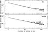 |
Fig. 7 Red-noise diagram for the residuals of the best-fitting model for SOI (top) and OSIRIS (bottom). Solid lines represent the rms calculated for a given bin width. Dashed lines show the expected behavior of the residuals for a pure Poisson-noise model. |
The determined parameters agree well with those reported by Bean et al. (2011) and Carter et al. (2011). We decided to decrease the number of free parameters in our MCMC fitting by fixing the values given by Bean et al. (2011), which are i = 88.94° and a/RS = 14.9749. This selection allowed us to directly compare the measured depth values with those reported in Désert et al. (2011), Croll et al. (2011), Bean et al. (2011), de Mooij et al. (2012), Murgas et al. (2012), Narita et al. (2013a,b), Fraine et al. (2013), and Teske et al. (2013).
The final de-trended light curves, the best-fitting transit-plus-trend models, and their residuals are shown in the middle and bottom panels in Figs. 1 and 2 for the OSIRIS and SOI observations, respectively. Low time-correlated noise in the SOI data is apparent in Fig. 7 (top).
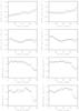 |
Fig. 8 First set of graphs (top four panels): changes in the distance between the target and comparison along the slit for two runs and two different wavelengths corresponding to center of the H and KS filters. The second set of plots (bottom four panels) depicts a ratio of FWHMs of the target and the comparison for first two runs for center pixels of H and KS wavelengths. |
3.2. Analysis of SofI data
First, we studied the main sources of systematic errors. One of our concerns was to understand how stable the centering of the target and the reference sources on the slit is. We measured the drifts and the full-width at half-maximum (FWHM) variations of both objects at two different wavelengths, corresponding to the H and K bands. The analysis consisted of the following steps: (i) determine the pixel corresponding to the center of the band; (ii) fit the spectral profiles at these wavelengths with Gaussian profiles to determine the center and FWHM of the two spectra. These steps were repeated independently for each good-weather run. The results for these runs are plotted in Fig. 8.
Apparently, the target-to-reference separation on the detector along the slit is stable to within 0.25 pixels (~0.007′′). We were unable to measure the positions of the stars across the slit with the same accuracy. Nevertheless, if we assume that the objects show the same relative drift in that direction as well, then the change of the flux ratio for two stars of similar brightness in the most extreme case, corresponding to a drift of 0.007′′ for one star while the other stays well centered on the slit, is about 0.2% for the whole run. The first run is slightly more stable. However, the monitoring of the separation along the slit indicates that it varies smoothly along the slit, without jumps, particularly, without dramatic jumps at the time of ingress and egress. This smooth variation is likely to occur due to color-dependent differential atmospheric refraction or smooth guider drift – mechanisms that are probably not related with the slit orientation. Therefore, we expect that the drift across the slit follows a similar smooth pattern.
The FWHM ratio (Fig. 8, bottom) also varies smoothly with time and is distinctly different from unity. The latter is related to the fixed position of the SofI collimator – for technical reasons it was not moved to adjust the focus for each set up. Instead, it was set at a position optimized for imaging observations, and the focus at spectroscopy is suboptimal, leading to a gradient across the FoV. This is the reason why the FWHM is different at the locations of the target and the reference stars. The effect of the suboptimal focus is more pronounced at the beginning of the observations at lower airmass, and weaker towards the end, when the higher airmass smears the images and makes the de-focusing less important.
Transit parameters of GJ 1214 b obtained from the SofI data.
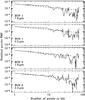 |
Fig. 9 Red-noise diagram for the residuals of the best-fitting model for SoFI data for two runs and two different wavelength channels. Solid lines represent the rms calculated for a given bin width. Dashed lines show the expected behavior of the residuals for a pure Poisson-noise model. |
The resulting light curve was analyzed via two different MCMC-based routines: one as described in previous section for our photometric data sets, and another based on the code by Gillon et al. (2009, 2012). Both methods provided consistent results. For clarity we present in the following text and in Table 3 the fitting parameters obtained with the second mentioned MCMC code described in Gillon et al. (2009, 2012). The rms of the residuals for different bin sizes are presented in Fig. 9. The transit is very short and the ingress/egress phase lasts only a few minutes. Therefore, the comparable bin size with comparable length of ingress/egress corresponds to binning of 2 or 3 points. Figure 9 suggests that the red-noise contribution to the overall error budget is fairly low. However, due to time sampling, it is not possible to draw a more accurate conclusion.
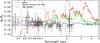 |
Fig. 10 Updated best fit atmospheric models reported in Miller-Ricci Kempton et al. (2012), including all current observational data. The models shown were smoothed for the sake of clarity. Light-gray points represent spectrophotometric measurements, and dark-gray points represent photometric measurements. The horizontal extension of the bars represents the wavelength coverage of the point, instead of an error associated with the observation. Black points represent our SOAR measurements. The dashed windows represent the zoomed-in regions displayed in Fig. 11. This figure is available in color in electronic form. |
4. Discussion
4.1. Spectrophotometric observations
The careful analysis shows that SOFI is fairly stable in terms of differential flux losses, and the duty cycle was extremely high −95–97%, that is, we lost only 3–5% of the time for detector readout, fits-file merging, and transferring. Unfortunately, the loss of the third night because of poor weather conditions undermined the analysis of our spectroscopic data, and the brightness of the exoplanet host was marginal. We still present the data here as a benchmark and reference for similar future observations, to demonstrate the potential of long-slit spectrographs at 4-m class telescopes to study extrasolar planets (e.g. Crossfield et al. 2013).
SOFI has a major advantage over other spectrographs: its long slit length of ~5′, which facilitates finding a suitable comparison star, which is necessary to control the systematics (see discussion in previous section and Fig. 9). Therefore, we conclude that SOFI is suitable for studying exoplanet atmospheres, if the planets orbit brighter stars.
4.2. Photometric GJ 1214 b atmosphere
A variety of measurements of the effective planet-to-star radius ratio at various wavelengths have provided conflicting clues on the composition of the GJ 1214b’s atmosphere. The first detections of this planet suggested that its radius is too large to be explained by a solid (pure rock or pure ice) composition (e.g., Charbonneau et al. 2009), implying the presence of a significant gaseous atmosphere. Depending on the assumptions made for the composition of the planet’s interior, this atmosphere could be composed primarily of hydrogen, water, or some combination thereof, a hypothesis that cannot be probed from a single radius measurement.
More recent detections at different wavelengths have suggested a high molecular weight atmosphere with a probable dominance of water, which would show shallow K-band depths (e.g., Bean et al. 2010, 2011; Désert et al. 2011; Berta et al. 2012). At the same time, Croll et al. (2011) reported a deep KS-band transit, which favors a low molecular weight atmosphere, with an hydrogen-rich component; this result was accompanied by the relatively deep KS-band transit reported by de Mooij et al. (2012). Meanwhile, Crossfield et al. (2011) reported that the hydrogen-rich atmosphere is not favored by their results. As noted by Howe & Burrows (2012), the shorter wavelength measurements reported by Bean et al. (2011) and de Mooij et al. (2012) favor hydrogen-rich atmospheres as well.
Nettelmann et al. (2011) considered different models for GJ 1214b’s interior, inferring metal-rich H/He atmospheres are the most plausible models, and suggesting an H/He/H2O model with a high water mass fraction for the atmosphere of the planet.
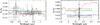 |
Fig. 11 Left: zoom-in from Fig. 10 for the optical region around our I-Bessel measurements. Right: K-band region of spectra around our 2.14 μm observation. Our measurement points are represented by dark circles, while gray points follow the description in Fig. 10. This figure is available in color in electronic form. |
There is no individual theoretical model that accounts for all the observational data, but atmospheres that either have a water-rich composition (more than 70% by mass) or a thick layer of clouds or hazes in the upper atmosphere are the best-suited interpretations of current data (e.g., Fortney 2005; Miller-Ricci & Fortney 2010; Nettelmann et al. 2011; Howe & Burrows 2012; Miller-Ricci Kempton et al. 2012). The last option has been studied by Morley et al. (2013), who found that in an enhanced metallicity atmosphere, clouds that formed either in chemical equilibrium or nonequilibrium frameworks can reproduce current observations. The authors also pointed out that hydrocarbon haze produced by photochemistry can flatten the GJ 1214 b spectrum.
Some studies have been performed to try to solve the discrepancies between the models. Murgas et al. (2012) used GTC tunable filters to attempt the detection of the Hα signature during transits of GJ 1214b, which yielded a nondetection, consistent with the featureless transmission spectra presented by Bean et al. (2011). Finally, Kreidberg et al. (2014) have provided strong evidence of the presence of clouds in the atmosphere of GJ 1214 b, based on HST transmission spectra. They reported the significant detection of a featureless spectrum, ruling out the cloud-free high molecular weight atmosphere hypothesis.
Figure 10 shows all current observational data that have a wavelength-dependent radius ratio, where the models correspond to updated best-fit atmosphere models proposed in Miller-Ricci Kempton et al. (2012). Photometric data were obtained from de Mooij et al. (2012, 2013), Carter et al. (2011), Bean et al. (2011), Murgas et al. (2012), Croll et al. (2011), Désert et al. (2011), Narita et al. (2013a,b), Teske et al. (2013), Colón & Gaidos (2013), Wilson et al. (2014), Gillon et al. (2014). Transmission spectroscopy measurements were obtained from Berta et al. (2012), Bean et al. (2011), and Kreidberg et al. (2014). Our measurement at 0.87 μm agrees well with current measurements at the shorter wavelengths, also suggesting the presence of the Rayleigh scattering tail argued in Howe & Burrows (2012). On the other hand, our NIR detection at 2.14 μm shows a moderate depth that disagrees with that of Croll et al. (2011) and the KS-band detection of Désert et al. (2011). Recently, Narita et al. (2013b) reported simultaneous J, H, and KS-band transit depths for transits of GJ 1214 b. Of particular interest is their shallow detection at 2.16 μm, which strongly disagrees with the deeper measurements. Our 2.14 μm detection is consistent with the detections of Narita et al. (2013b) and Bean et al. (2011) and the KC detection of Désert et al. (2011).
For better orientation, Fig. 11, left, is a zoom-in of Fig. 10 with a focus on the optical region around our SOI measurement, while the same Fig. 11, right, shows the NIR region around our OSIRIS measurement. For both panels, relevant measurements by the above mentioned groups are presented for comparison.
Finally, we would like to point out a discrepancy between the narrow-band and broad-band photometric measurements at similar wavelengths (see Fig. 11). Our measurement at 2.14 μm contrasts with the broad band measurements by Croll et al. (2011) and Narita et al. (2013b) and agrees well with the narrow-band measurement of de Mooij et al. (2012) at 2.27 μm.
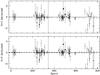 |
Fig. 12 Top: observed-minus-calculated (O–C) diagram for the whole set of transit timing available to date in the literature, calculated on the ephemeris given by Bean et al. (2011). Our measurements are drawn as filled squares and in addition highlighted by colors in the online version. The dashed line represents the new ephemeris calculated in this work. Bottom: same data set after removing the new ephemeris, including its 1-σ errors (dashed lines). |
4.3. Transit-timing observations
The timing information in the raw images was converted from MJD to BJD (TDB) to determine the final individual transit timing, following the prescriptions in Eastman et al. (2010). Our photometric data show no significant deviations from a constant period, which is consistent with what has been found by Carter et al. (2011) and Berta et al. (2012), and has been recently confirmed by Harpsøe et al. (2013), who used a Bayesian approach to infer that a TTV is unlikely to be present in the GJ 1214b data. We collected all available transit-timing data from the literature, which we combined with our measurements to refine the ephemeris of the GJ1214b system, with parameters T0 = 2 454 934.917003 ± 0.000023 BJD and P = 1.580404599 ± 0.000000056. Timing data from de Mooij et al. (2012), Kundurthy et al. (2011), Carter et al. (2011), Murgas et al. (2012), Bean et al. (2011), Charbonneau et al. (2009), Berta et al. (2011, 2012), Croll et al. (2011), Désert et al. (2011), Sada et al. (2010), Narita et al. (2013b), Harpsøe et al. (2013), Teske et al. (2013), Gillon et al. (2014), Colón & Gaidos (2013), Fraine et al. (2013), and our measurements are shown in Fig. 12.
Based on the timing analysis of GJ1214b transits, we put strong constraints on the mass of an additional body in the system, especially in mean motion resonances (MMRs) with the transiting exoplanet. Using dynamical simulations with the MERCURY N-body orbital integrator (Chambers 1999), we determined the mass of an orbital perturber as a function of the distance from the star. To run the simulations we followed the same procedure as described in detail in Hoyer et al. (2011). We used the updated physical parameters of the system reported by Anglada-Escudé et al. (2013) as input for the simulations. For the perturber body, we explored a wide range of masses (0.5 M⊕–1000 M⊕) and orbital distances (0.0015 AU–0.055 AU), searching for the masses that produce an rms of ~30 s in the calculated central time of the transits of GJ1214b during the ten years of integration time we used. The results of these dynamical simulations are presented in Fig. 13 where a region of unstable orbits is marked by the gray strip. For all the other stable orbits we determined the perturber mass that would produce a TTV rms of 30 s (represented by the solid line). In the 1:2, 2:3 (interior), and in the 3:2, 2:1 (exterior) MMRs (vertical lines in Fig. 13) the upper mass limits we obtained correspond to ~0.5 M⊕. These are better constraints in the mass of a possible companion of GJ 1214 b than the limits imposed by radial velocity measurements.
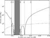 |
Fig. 13 Upper mass limits for the system GJ 1214b based on numerical simulations. The dashed line represents the limits imposed by the radial velocity measurements. |
5. Summary
GJ 1214 b is undoubtedly one of the most intriguing objects and the first of its class with an extensively studied atmosphere. The NIR and optical photometric measurements we present here provide additional evidence for a rather flat featureless spectrum, indicating either a metal-rich, or a cloudy or hazy atmosphere. The TTV analysis of our data combined with previous data sets by other groups have confirmed the constant value of the planetary orbital period.
All observations reported here were performed with 4m class telescopes and prove the suitability of such facilities for high-precision photometry. Furthermore, we encourage new spectroscopic measurements especially in the H and Ks bands of the spectra. Particularly suitable instruments are either multi-object spectrographs or, as presented in this paper, long-slit spectrographs with very wide and long slits capable of simultaneously monitoring a comparison star. In the latter case, 4m class telescope usage as for GJ1214b may be challenging, but might provide very interesting results for multiple events.
IRAF is distributed by the NOAO, which are operated by the AURA in Astronomy, Inc., under cooperative agreement with the NSF.
Acknowledgments
The authors are grateful to the SOAR and the ESO staff for the help during the observations. The SOI observations were performed thanks to granted Director’s Discretionary Time of the SOAR Telescope. C.C. acknowledges support from ALMA-CONICYT Fund through grant 31100025 and project CONICYT FONDECYT Postdoctorado 3140592. SH and PR would like to acknowledge grant FONDECYT 1120299. S.H. also acknowledges financial support from the Spanish Ministry of Economy and Competitiveness (MINECO) under the 2011 Severo Ochoa Program MINECO SEV-2011-0187. P.K. acknowledges co-funding under the Marie Curie Actions of the European Commission (FP7-COFUND) and the MCMC code kindly provided by Michäel Gillon (University of Liège). D.M. thanks Basal-CATA PFB-06.
References
- Anglada-Escudé, G., Rojas-Ayala, B., Boss, A. P., Weinberger, A. J., & Lloyd, J. P. 2013, A&A, 551, A48 [NASA ADS] [CrossRef] [EDP Sciences] [Google Scholar]
- Bean, J. L., Miller-Ricci Kempton, E., & Homeier, D. 2010, Nature, 468, 669 [NASA ADS] [CrossRef] [PubMed] [Google Scholar]
- Bean, J. L., Désert, J.-M., Kabath, P., et al. 2011, ApJ, 743, 92 [NASA ADS] [CrossRef] [Google Scholar]
- Berta, Z. K., Charbonneau, D., Bean, J., et al. 2011, ApJ, 736, 12 [NASA ADS] [CrossRef] [Google Scholar]
- Berta, Z. K., Charbonneau, D., Désert, J.-M., et al. 2012, ApJ, 747, 35 [NASA ADS] [CrossRef] [Google Scholar]
- Cáceres, C., Ivanov, V. D., Minniti, D., et al. 2009, A&A, 507, 481 [NASA ADS] [CrossRef] [EDP Sciences] [Google Scholar]
- Cáceres, C., Ivanov, V. D., Minniti, D., et al. 2011, A&A, 530, A5 [NASA ADS] [CrossRef] [EDP Sciences] [Google Scholar]
- Carter, J. A., Winn, J. N., Holman, M. J., et al. 2011, ApJ, 730, 82 [NASA ADS] [CrossRef] [Google Scholar]
- Chambers, J. E. 1999, MNRAS, 304, 793 [NASA ADS] [CrossRef] [MathSciNet] [Google Scholar]
- Charbonneau, D., Berta, Z. K., Irwin, J., et al. 2009, Nature, 462, 891 [NASA ADS] [CrossRef] [PubMed] [Google Scholar]
- Claret, A., & Bloemen, S. 2011, A&A, 529, A75 [NASA ADS] [CrossRef] [EDP Sciences] [Google Scholar]
- Collier Cameron, A., Wilson, D. M., West, R. G., et al. 2007, MNRAS, 380, 1230 [NASA ADS] [CrossRef] [Google Scholar]
- Colón, K. D., & Gaidos, E. 2013, ApJ, 776, 49 [NASA ADS] [CrossRef] [Google Scholar]
- Croll, B., Albert, L., Jayawardhana, R., et al. 2011, ApJ, 736, 78 [NASA ADS] [CrossRef] [Google Scholar]
- Crossfield, I. J. M., Barman, T., & Hansen, B. M. S. 2011, ApJ, 736, 132 [NASA ADS] [CrossRef] [Google Scholar]
- Crossfield, I. J. M., Barman, T., Hansen, B. M. S., & Howard, A. W. 2013, A&A, 559, A33 [NASA ADS] [CrossRef] [EDP Sciences] [Google Scholar]
- de Mooij, E. J. W., Brogi, M., de Kok, R. J., et al. 2012, A&A, 538, A46 [NASA ADS] [CrossRef] [EDP Sciences] [Google Scholar]
- de Mooij, E. J. W., Brogi, M., de Kok, R. J., et al. 2013, ApJ, 771, 109 [NASA ADS] [CrossRef] [Google Scholar]
- Depoy, D. L., Atwood, B., Byard, P. L., Frogel, J., & O’Brien, T. P. 1993, in SPIE Proc. 1946, eds. A. M. Fowler, 667 [Google Scholar]
- Désert, J.-M., Bean, J., Miller-Ricci Kempton, E., et al. 2011, ApJ, 731, L40 [NASA ADS] [CrossRef] [Google Scholar]
- Eastman, J., Siverd, R., & Gaudi, B. S. 2010, PASP, 122, 935 [NASA ADS] [CrossRef] [Google Scholar]
- Ford, E. B. 2005, AJ, 129, 1706 [Google Scholar]
- Ford, E. B. 2006, ApJ, 642, 505 [NASA ADS] [CrossRef] [Google Scholar]
- Fortney, J. J. 2005, MNRAS, 364, 649 [NASA ADS] [CrossRef] [Google Scholar]
- Fraine, J. D., Deming, D., Gillon, M., et al. 2012, in AAS/Division for Planetary Sciences Meeting Abstracts, 44, 01304 [Google Scholar]
- Fraine, J. D., Deming, D., Gillon, M., et al. 2013, ApJ, 765, 127 [NASA ADS] [CrossRef] [Google Scholar]
- Gelman, A., & Rubin, D. 1992, Statist. Sci., 7, 457 [NASA ADS] [CrossRef] [Google Scholar]
- Gillon, M., Pont, F., Moutou, C., et al. 2006, A&A, 459, 249 [NASA ADS] [CrossRef] [EDP Sciences] [Google Scholar]
- Gillon, M., Demory, B.-O., Triaud, A. H. M. J., et al. 2009, A&A, 506, 359 [NASA ADS] [CrossRef] [EDP Sciences] [Google Scholar]
- Gillon, M., Lanotte, A. A., Barman, T., et al. 2010, A&A, 511, A3 [NASA ADS] [CrossRef] [EDP Sciences] [Google Scholar]
- Gillon, M., Triaud, H. M. J. A., Fortney, J. J., et al. 2012, A&A, 542, A3 [Google Scholar]
- Gillon, M., Demory, B.-O., Madhusudhan, N., et al. 2014, A&A, 563, A21 [NASA ADS] [CrossRef] [EDP Sciences] [Google Scholar]
- Gregory, P. C. 2005, ApJ, 631, 1198 [NASA ADS] [CrossRef] [Google Scholar]
- Harpsøe, K. B. W., Hardis, S., Hinse, T. C., et al. 2013, A&A, 549, A10 [Google Scholar]
- Holman, M. J., Winn, J. N., Latham, D. W., et al. 2006, ApJ, 652, 1715 [NASA ADS] [CrossRef] [Google Scholar]
- Howe, A. R., & Burrows, A. S. 2012, ApJ, 756, 176 [NASA ADS] [CrossRef] [Google Scholar]
- Hoyer, S., Rojo, P., López-Morales, M., et al. 2011, ApJ, 733, 53 [NASA ADS] [CrossRef] [Google Scholar]
- Hoyer, S., Rojo, P., & López-Morales, M. 2012, ApJ, 748, 22 [NASA ADS] [CrossRef] [Google Scholar]
- Kreidberg, L., Bean, J. L., Désert, J.-M., et al. 2014, Nature, 505, 69 [NASA ADS] [CrossRef] [Google Scholar]
- Kundurthy, P., Agol, E., Becker, A. C., et al. 2011, ApJ, 731, 123 [NASA ADS] [CrossRef] [Google Scholar]
- Mandel, K., & Agol, E. 2002, ApJ, 580, L171 [NASA ADS] [CrossRef] [Google Scholar]
- Miller-Ricci, E., & Fortney, J. J. 2010, ApJ, 716, L74 [NASA ADS] [CrossRef] [Google Scholar]
- Miller-Ricci Kempton, E., Zahnle, K., & Fortney, J. J. 2012, ApJ, 745, 3 [Google Scholar]
- Moorwood, A., Cuby, J.-G., & Lidman, C. 1998, The Messenger, 91, 9 [NASA ADS] [Google Scholar]
- Morley, C. V., Fortney, J. J., Kempton, E. M.-R., et al. 2013, ApJ, 775, 33 [NASA ADS] [CrossRef] [Google Scholar]
- Murgas, F., Pallé, E., Cabrera-Lavers, A., et al. 2012, A&A, 544, A41 [NASA ADS] [CrossRef] [EDP Sciences] [Google Scholar]
- Narita, N., Fukui, A., Ikoma, M., et al. 2013a, ApJ, 773, 144 [NASA ADS] [CrossRef] [Google Scholar]
- Narita, N., Nagayama, T., Suenaga, T., et al. 2013b, PASJ, 65, 27 [NASA ADS] [Google Scholar]
- Nettelmann, N., Fortney, J. J., Kramm, U., & Redmer, R. 2011, ApJ, 733, 2 [Google Scholar]
- Press, W. H., Teukolsky, S. A., Vetterling, W. T., & Flannery, B. P. 1992, Numerical recipes in C. The art of scientific computing (Cambridge: University Press) [Google Scholar]
- Rogers, L. A., & Seager, S. 2010, ApJ, 716, 1208 [NASA ADS] [CrossRef] [Google Scholar]
- Sada, P. V., Deming, D., Jackson, B., et al. 2010, ApJ, 720, L215 [NASA ADS] [CrossRef] [Google Scholar]
- Tegmark, M., Strauss, M. A., Blanton, M. R., et al. 2004, Phys. Rev. D, 69, 103501 [CrossRef] [Google Scholar]
- Teske, J. K., Turner, J. D., Mueller, M., & Griffith, C. A. 2013, MNRAS, 431, 1669 [NASA ADS] [CrossRef] [Google Scholar]
- Wilson, P. A., Colón, K. D., Sing, D. K., et al. 2014, MNRAS, 438, 2395 [NASA ADS] [CrossRef] [Google Scholar]
- Winn, J. N., Holman, M. J., Torres, G., et al. 2008, ApJ, 683, 1076 [NASA ADS] [CrossRef] [Google Scholar]
All Tables
All Figures
|
Fig. 1 2.14 μm GJ 1214 b photometric series obtained with OSIRIS. Top: raw light curve, with the best-fitting transit model in red. Middle: de-trended light curve with the best-fitting model. Bottom: residuals from the best-fitting model; the rms. is 0.0062. This figure is available in color in electronic form. |
| In the text | |
|
Fig. 2 I-Bessel GJ 1214 b photometric series obtained with SOI. Top: raw light curve, with the best-fitting transit model in red. Middle: de-trended light curve with the best-fitting model. Bottom: residuals from the best-fitting model; the rms is 0.0019. This figure is available in color in electronic form. |
| In the text | |
|
Fig. 3 Typical wavelength-calibrated one-dimensional spectrum of GJ 1214 b, not corrected for telluric absorption, obtained with SofI on May 17/18, 2011. |
| In the text | |
|
Fig. 4 Spectrophotometric individual time series obtained from integrating the flux of the SofI spectra within the H and KS bands for the target and its comparison stars, and for the two good-weather runs. |
| In the text | |
|
Fig. 5 H (1.6 μm) and KS (2.2 μm) GJ 1214 b spectrophotometric series obtained from integrating the flux of the SofI spectra within the H and KS bands. Top: raw light curves, with the best-fitting transit models in red. Bottom: de-trended light curves with the best-fitting models. This figure is available in color in electronic form. |
| In the text | |
|
Fig. 6 Parameters used to de-trend the OSIRIS photometric time series. From top to bottom: sky flux value and (ΔxC,ΔyC), the variations of the target’s position coordinates around their median value. |
| In the text | |
|
Fig. 7 Red-noise diagram for the residuals of the best-fitting model for SOI (top) and OSIRIS (bottom). Solid lines represent the rms calculated for a given bin width. Dashed lines show the expected behavior of the residuals for a pure Poisson-noise model. |
| In the text | |
|
Fig. 8 First set of graphs (top four panels): changes in the distance between the target and comparison along the slit for two runs and two different wavelengths corresponding to center of the H and KS filters. The second set of plots (bottom four panels) depicts a ratio of FWHMs of the target and the comparison for first two runs for center pixels of H and KS wavelengths. |
| In the text | |
|
Fig. 9 Red-noise diagram for the residuals of the best-fitting model for SoFI data for two runs and two different wavelength channels. Solid lines represent the rms calculated for a given bin width. Dashed lines show the expected behavior of the residuals for a pure Poisson-noise model. |
| In the text | |
|
Fig. 10 Updated best fit atmospheric models reported in Miller-Ricci Kempton et al. (2012), including all current observational data. The models shown were smoothed for the sake of clarity. Light-gray points represent spectrophotometric measurements, and dark-gray points represent photometric measurements. The horizontal extension of the bars represents the wavelength coverage of the point, instead of an error associated with the observation. Black points represent our SOAR measurements. The dashed windows represent the zoomed-in regions displayed in Fig. 11. This figure is available in color in electronic form. |
| In the text | |
|
Fig. 11 Left: zoom-in from Fig. 10 for the optical region around our I-Bessel measurements. Right: K-band region of spectra around our 2.14 μm observation. Our measurement points are represented by dark circles, while gray points follow the description in Fig. 10. This figure is available in color in electronic form. |
| In the text | |
|
Fig. 12 Top: observed-minus-calculated (O–C) diagram for the whole set of transit timing available to date in the literature, calculated on the ephemeris given by Bean et al. (2011). Our measurements are drawn as filled squares and in addition highlighted by colors in the online version. The dashed line represents the new ephemeris calculated in this work. Bottom: same data set after removing the new ephemeris, including its 1-σ errors (dashed lines). |
| In the text | |
|
Fig. 13 Upper mass limits for the system GJ 1214b based on numerical simulations. The dashed line represents the limits imposed by the radial velocity measurements. |
| In the text | |
Current usage metrics show cumulative count of Article Views (full-text article views including HTML views, PDF and ePub downloads, according to the available data) and Abstracts Views on Vision4Press platform.
Data correspond to usage on the plateform after 2015. The current usage metrics is available 48-96 hours after online publication and is updated daily on week days.
Initial download of the metrics may take a while.