| Issue |
A&A
Volume 564, April 2014
|
|
|---|---|---|
| Article Number | A86 | |
| Number of page(s) | 8 | |
| Section | The Sun | |
| DOI | https://doi.org/10.1051/0004-6361/201323143 | |
| Published online | 10 April 2014 | |
Energy and helicity budgets of solar quiet regions
1
Research Center for Astronomy and Applied Mathematics, Academy of
Athens,
4 Soranou Efesiou Street,
Athens
11527,
Greece
e-mail:
This email address is being protected from spambots. You need JavaScript enabled to view it.
2
Institute for Astronomy, Astrophysics, Space Applications and
Remote Sensing, National Observatory of Athens, 15236
Penteli,
Greece
Received:
28
November
2013
Accepted:
28
February
2014
Abstract
Aims. We investigate the free magnetic energy and relative magnetic helicity budgets of solar quiet regions.
Methods. Using a novel nonlinear force-free method that requires single solar vector magnetograms we calculated the instantaneous free magnetic energy and relative magnetic helicity budgets in 55 quiet-Sun vector magnetograms.
Results. As in a previous work on active regions, we constructed here for the first time the (free) energy-(relative) helicity diagram of quiet-Sun regions. We find that quiet-Sun regions have no dominant sense of helicity and show monotonic correlations a) between free magnetic energy/relative helicity and magnetic network area and, consequently, b) between free magnetic energy and helicity. Free magnetic energy budgets of quiet-Sun regions represent a rather continuous extension of respective active-region budgets towards lower values, but the corresponding helicity transition is discontinuous because of the incoherence of the helicity sense in contrast to active regions. We furthermore estimated the instantaneous free magnetic-energy and relative magnetic-helicity budgets of the entire quiet Sun, as well as the respective budgets over an entire solar cycle.
Conclusions. Derived instantaneous free magnetic energy budgets and, to a lesser extent, relative magnetic helicity budgets over the entire quiet Sun are similar to the respective budgets of a sizeable active region, while total budgets within a solar cycle are found to be higher than previously reported. Free-energy budgets are similar to the energy needed to power fine-scale structures residing at the network, such as mottles and spicules.
Key words: Sun: chromosphere / Sun: magnetic fields / Sun: photosphere
© ESO, 2014
1. Introduction
Free magnetic energy corresponds to the excess energy of any magnetic region from its “ground”, current-free (potential) energy state, while magnetic helicity quantifies the stress and distortion of the magnetic field lines compared with their potential-energy state. Free magnetic energy builds up mainly through continuous flux emergence on the solar surface and other processes such as coronal interactions (e.g. fly-bys, Galsgaard et al. 2000) or photospheric twisting (e.g. Pariat et al. 2009). Magnetic helicity either emerges from the solar interior via helical magnetic flux tubes or is being generated by solar differential rotation and peculiar photospheric motions.
In solar active regions (ARs) considerable localized magnetic flux emergence on the order of 1022 Mx (Schrijver & Harvey 1994) builds up strong opposite-polarity regions that are sometimes separated by intense, highly sheared polarity inversion lines (PILs), hence deviate substantially from a potential-field configuration. ARs tend to store large amounts of both free magnetic energy and magnetic helicity. Free magnetic energy is released, via magnetic reconnection events, in solar flares and/or coronal mass ejections (CMEs). Helicity, however, cannot be efficiently removed by magnetic reconnection (Berger 1984), and if not transferred to larger scales via existing magnetic connections, it can only be expelled in the form of CMEs (Low 1994; DeVore 2000). The role of both free magnetic energy and helicity in ARs has been recently investigated by Georgoulis et al. (2012) and Tziotziou et al. (2012, 2013).
On the other hand, quiet-Sun regions are dominated by the flow pattern of large convective cells called supergranules that range in diameter from 10 000 km to 50 000 km, with an average diameter between 13 000 and 18 000 km (Hagenaar et al. 1997). High-resolution magnetograms show continuous emergence of new bipolar elements inside the cell interiors, called the internetwork (IN), that are swept by the supergranular flow towards the boundaries of supergranular cells where opposite polarity fluxes cancel, whereas like-polarity fluxes merge (Wang et al. 1996; Schrijver et al. 1997). By this process hierarchic flux concentrations are formed at the intersection of supergranular cells. These magnetic flux concentrations, which are characterized by magnetic fluxes on the order of 1018–1019 Mx and typical diameters of 1000–10 000 km (Parnell 2001), constitute the so-called magnetic network. Free magnetic energy, released in the network mainly by reconnection, can fuel the dynamics of several small-scale structures, such as mottles/spicules, which reside there and are governed by the dynamics and physics of the network magnetic field (see the review by Tsiropoula et al. 2012, for further details). Free magnetic energy release from nonpotential magnetic configurations in the quiet Sun has also been reported to result in small-scale structures, such as bright points (Zhao et al. 2009), blinkers (Woodard & Chae 1999) and quiet-Sun corona nanoflares (Meyer et al. 2013). There are no reports in the literature concerning the accumulation and expulsion of relative magnetic helicity in the magnetic network and quiet-Sun regions in general and this mechanism’s role in quiet-Sun dynamics; only Zhao et al. (2009) have investigated current helicity budgets in network bright points. However, there exist reports (Jess et al. 2009; Curdt & Tian 2011; De Pontieu et al. 2012) that argue for torsional oscillations in fine structures, such as explosive events and spicules, thus suggesting the existence of twisting motions that could lead to expulsion or transfer of helicity to larger scales in the solar atmosphere.
Until recently, no robust method existed to calculate the instantaneous free magnetic energy and relative magnetic helicity budgets of a solar region. Existing methods were based either on integration in time of an energy/helicity injection rate (Berger & Field 1984) or on evaluation of classical formulas (hereafter volume calculations, Finn & Antonsen 1985; Berger 1999) using a three-dimensional magnetic field derived from extrapolations. However, energy/helicity injection rates depend on the determination of the photospheric velocity field, which involves significant uncertainties (e.g., Welsch et al. 2007). On the other hand, volume calculations depend on model-dependent nonlinear force-free (NLFF) field extrapolations that also carry several uncertainties and ambiguities (e.g., Schrijver et al. 2006; Metcalf et al. 2008,and references therein). Recently, Georgoulis et al. (2012) proposed a novel NLFF method to calculate the instantaneous magnetic free energy and relative helicity budgets from a single (photospheric or chromospheric) vector magnetogram. The method was used for calculating the free magnetic energy and relative helicity budgets in solar ARs (Georgoulis et al. 2012; Tziotziou et al. 2013) and for deriving the energy-helicity diagram of solar ARs (Tziotziou et al. 2012). The latter shows a nearly monotonic dependence between the two quantities.
The aim of this paper is to a) derive the instantaneous budgets of free magnetic energy and relative magnetic helicity in quiet-Sun regions using the NLFF method, b) construct the corresponding energy-helicity diagram and compare it with the respective diagram for ARs, and c) calculate available budgets of free energy and helicity over an entire solar cycle and associate them with the energetics and dynamics of fine-scale quiet-Sun structures. Section 2 briefly describes and discusses the observations and the methodology, Sect. 3 presents the results, while Sect. 4 discusses the results and summarizes our findings.
2. Observations and methodology
2.1. Observations
For our analysis we used a sizable sample of photospheric vector magnetograms of quiet-Sun regions obtained by the space-borne Spectropolarimeter (SP; see description in Lites et al. 2008) of the Solar Optical Telescope (SOT) onboard the Hinode satellite. SP provides full Stokes profiles of the Fe I 630.25/630.15 nm lines with a maximum spatial sampling of 0.16′′ per pixel. All vector magnetograms were treated for the azimuthal 180° ambiguity by means of the nonpotential field calculation (NPFC) of Georgoulis (2005), as revised in Metcalf et al. (2006). For our analysis we used the heliographic components of the magnetic field vector on the heliographic plane, derived with the de-projection equations of Gary & Hagyard (1990). As typical uncertainties for the line-of-sight and transverse field components of SOT/SP data we used (δBl, δBtr) = (5, 50) G.
A total of 132 quiet-Sun regions, observed between 2006 and 2011 when the Sun was mostly quiet, were initially examined. Of these, we selected 55 magnetograms that exhibited an overall flux imbalance not exceeding 15%, with an average imbalance of about 5%. This is because our NLFF calculation gives more reliable results in flux-balanced environments. The spatial resolution of the analyzed magnetograms is 0.16′′ or 0.32′′ per pixel and Fig. 1 shows the spatial distribution of these regions on the solar disk. The majority of them is located close to the solar disk center and cover a sizeable area of the solar surface; areas on the image plane range between 1 426 and 86 088 arcsec2, with a mean area size of 32 078 arcsec2.
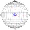 |
Fig. 1 Central heliographic positions for the 55 vector quiet-Sun magnetograms included in our analysis. The size of the diamonds implies normalized (to the maximum value) area size. Red/blue diamonds correspond to negative/positive total magnetic helicity budgets (see Sect. 3.1). |
Figure 2 (top panel) shows an example of an SOT/SP magnetogram used in this analysis. As the figure shows, the magnetic field is mostly concentrated at the boundaries of the supergranular cells that constitute the magnetic network.
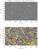 |
Fig. 2 Top panel: an observed SOT/SP magnetogram (vertical field component Bz) of a quiet-Sun region studied here. White/black denotes positive/negative magnetic field concentrations. Bottom panel: inferred magnetic connectivity of the region, showing the vertical magnetic field component in grayscale with the contours bounding the identified magnetic partitions. The flux-tube connections identified by the magnetic connectivity matrix are represented by line segments connecting the flux-weighted centroids of the respective pair of partitions. Red, blue, yellow, and cyan segments denote magnetic flux contents within the ranges [1016, 1017] Mx, [1017, 1018] Mx, [1018, 1019] Mx, and >1019 Mx, respectively. Only connections closing within the field-of-view are shown. |
2.2. Methodology for calculating magnetic energy and helicity budgets
The method for deriving the instantaneous free magnetic-energy and relative magnetic-helicity budgets is the recently proposed NLFF method by Georgoulis et al. (2012) that uses a single photospheric or chromospheric vector magnetogram. In contrast to model-dependent NLFF field extrapolation methods, it provides unique results relying on a unique magnetic-connectivity matrix that contains the flux committed to connections between positive- and negative-polarity flux partitions. Since the three-dimensional magnetic configuration is unknown, the connectivity matrix is derived by means of a simulated annealing method (Georgoulis & Rust 2007; Georgoulis et al. 2012). This method guarantees connections between opposite-polarity flux partitions while globally (within the field-of-view) minimizing the corresponding connection lengths. The nonzero flux elements of the derived connectivity matrix define a collection of N magnetic connections, which are treated as slender force-free flux tubes with known footpoints, flux contents, and variable force-free parameters.
For flux tubes that do not wind around each other’s axes, as Georgoulis et al. (2012) have shown, the lower-limit free magnetic
energy Ec can be expressed as the sum of two
terms: a self-term Ecself, describing the
internal twist and writhe of each flux tube, and a mutual term Ecmut, describing interactions
between different flux tubes. Ec is defined by 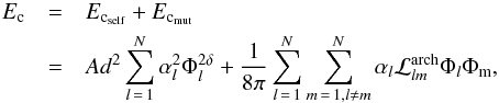 (1)where
d is the
pixel size of the magnetogram, A and δ are known fitting constants, and Φl and
αl are the respective
unsigned flux and force-free parameters of flux tube l.
(1)where
d is the
pixel size of the magnetogram, A and δ are known fitting constants, and Φl and
αl are the respective
unsigned flux and force-free parameters of flux tube l.
 is the
mutual-helicity factor of two arch-like flux tubes, which was first introduced by Demoulin et al. (2006) and was subsequently analyzed by
Georgoulis et al. (2012) for all possible cases.
Since the winding factor (Gauss linking number) around flux tubes is unknown and hence set
to zero, the derived free energy always represents a lower, but realistic limit (Georgoulis et al. 2012; Tziotziou et al. 2012).
is the
mutual-helicity factor of two arch-like flux tubes, which was first introduced by Demoulin et al. (2006) and was subsequently analyzed by
Georgoulis et al. (2012) for all possible cases.
Since the winding factor (Gauss linking number) around flux tubes is unknown and hence set
to zero, the derived free energy always represents a lower, but realistic limit (Georgoulis et al. 2012; Tziotziou et al. 2012).
Likewise, the corresponding relative magnetic helicity Hm is the sum of
a self Hmself and a mutual
Hmmut term, namely
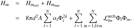 (2)Derivation
of uncertainties for all terms of Eqs. (1)
and (2) is fully described in Georgoulis et al. (2012).
(2)Derivation
of uncertainties for all terms of Eqs. (1)
and (2) is fully described in Georgoulis et al. (2012).
Figure 2 (bottom panel) shows the inferred connectivity matrix for the quiet-Sun region shown in the top panel. Positive/negative partitions are, as expected, mostly concentrated in supergranular boundaries (magnetic network), where considerable concentrations of magnetic flux are observed. Moreover, connections are mostly between nearby opposite-polarity partitions as a result of the used simulated annealing method.
2.2.1. Validity of the method
Georgoulis et al. (2012) discussed in detail (see their Sect. 2.3) the validity of this method for potential-field configurations. The authors argued that nonpotentiality of the studied region is a necessary assumption to derive the magnetic connectivity matrix with simulated annealing, since it strongly favors PILs. And if nonpotentiality characterizes solar active regions (e.g., Zirin & Wang 1993; Leka et al. 1996), this is not the case for quiet-Sun regions, which are widely believed to be close to a potential-field configuration and have mostly been treated as such (e.g., Kontogiannis et al. 2010, 2011; Wiegelmann et al. 2013). However, there exist observations and modeling that suggest the existence of nonpotential fields within the quiet-Sun and its magnetic network (Woodard & Chae 1999; Zhao et al. 2009; Liu et al. 2011; Uritsky et al. 2013; Meyer et al. 2013; Chesny et al. 2013).
Furthermore, there are a few elements characterizing the magnetic field configuration of the quiet Sun that would still allow using simulated annealing. First, an observed quiet-Sun magnetogram is usually not flux-balanced. As a result, mutual-helicity terms could still add up to give considerable helicity values when free magnetic energy tends to zero due to the very small, close to zero, values of αl in Eq. (1), because electric currents are almost absent. Indeed, our results (see Figs. 4 and 6 and relevant discussion) indicate that free magnetic energy acquires very low values compared with those for ARs. Second, the quiet-Sun magnetic field concentrates on hierarchical structures (network). And even though there are no strong PILs present in quiet-Sun magnetograms, the supergranular cell configuration of the network favors an essential ingredient of the used simulated annealing, that is, simultaneous minimization of the flux imbalance and the separation length between chosen partitions, with the latter often being shorter than the supergranular cell radius (see Fig. 2).
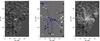 |
Fig. 3 Left panel: an Hα image observed with the Dutch Open Telescope (see Kontogiannis et al. 2010, for details). Middle panel: corresponding SOT/SP magnetogram (vertical field component Bz) of the quiet-Sun region with the inferred connectivity overlaid (see caption of Fig. 2 for an explanation of the magnetic connectivity matrix). Right panel: field lines of the potential field extrapolation of Kontogiannis et al. (2010, their Fig. 2) overlaid on the Hα image of the left panel. |
Figure 3 shows an Hα quiet-Sun region (left panel) and its SOT/SP magnetogram (middle panel) that was studied by Kontogiannis et al. (2010). They calculated the potential magnetic field of the chromosphere, and in their Fig. 2 (potential case hereafter), the magnetic field lines were plotted over an Hα average image that is part of the one shown in Fig. 3, rotated by 26°, and shown here for direct comparison in the right panel of Fig. 3. This gives us the opportunity to compare between the magnetic connectivity as calculated for a potential magnetic field and by the annealing method used in this paper. This very quiet solar region is located almost at the disk center. Two major positive-polarity clusters stand out, which reach 1 kG, and some negative and positive ones with lower strength (a few hundred G), while several mixed-polarity elements are scattered across the IN. We note, however, that the signed magnetic flux is predominantly positive (45% imbalance) and the annealing method takes into account only partitions with fluxes above a certain threshold.
In the potential case, the two positive-polarity network clusters connect partly with the negative polarity elements at the middle-right of the field-of-view (FOV) and with several negative magnetic elements at the IN. The bundles of field lines coincide nicely with the absorption features in Hα. For the most part the same connectivity is inferred from our method (Fig. 3, middle panel), but at a lower detail because the imposed threshold excludes very weak partitions. However, most of the connections (if not all) with the IN are lost. At the left of the cluster, parallel field lines connect weak opposite polarities and appear as a chain of mottles in Hα. This structure is not found in the middle panel of Fig. 3: only the strongest negative partitions are detected and they are connected with the network cluster. Several small-scale flux tubes, formed at the IN, in the vicinity (or at places) of Hα absorption, are also lacking. Some very long potential magnetic field lines connect the network with remote magnetic elements; these connections are also found here and the inferred flux tubes match the general orientation of absorption features, even though such long flux tubes are not usually observed in Hα.
As a concluding remark, our flux threshold, which is necessary to calculate the flux tubes that connect opposite-polarity elements, results in missing the finest magnetic fields of the internetwork. Moreover, several other possible connections are lacking as a result of the non-flux-balanced FOV. However, the method reproduces the general configuration inferred from Hα observations.
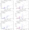 |
Fig. 4 Derived free magnetic energy (left column) and relative magnetic helicity (right column) budgets as a function of the image plane magnetic network area for three different network area thresholds of 100 G, 200 G, and 300 G. In plots involving helicity budgets, red/blue colors correspond to negative/positive magnetic-helicity budgets. Quiet-Sun regions centered within latitudes of ±30° (see Fig. 1) are represented by asterisks, while regions centered on larger latitudes are presented by diamonds. Error bars in helicity are also shown, while respective energy errors are not indicated because of their very small amplitude (~1028 erg). Dashed lines show the best linear fit between helicity/energy and network area (y = A + Bx, where y represents helicity/energy and x the network area). Derived fitting coefficients A and B, the goodness of the fit r, as well as the mean network area as a percentage of the magnetogram area are also registered within each plot. Derived linear fit coefficients (A,B) between free magnetic energy and heliographic plane network area are equal to (−2.89 × 1029, 4.33 × 1026), (− 2.53 × 1029, 9.39 × 1026), and (−2.21 × 1029, 1.42 × 1027) for the three network thresholds, while for relative magnetic helicity and heliographic plane network area they are equal to (−5.06 × 1037, 7.89 × 1035), (−5.63 × 1037, 2.31 × 1036), and (−6.53 × 1035, 3.54 × 1036). |
3. Results
3.1. Energy and helicity budgets of quiet-Sun regions
Using Eqs. (1) and (2), we derived the free magnetic energy and relative magnetic helicity budgets for the selected 55 quiet-Sun vector magnetograms. The free magnetic energy ranges between 7.5 × 1026 erg and 4.8 × 1030 erg, while the relative magnetic helicity ranges between 7.53 × 1036 Mx2 and 1.4 × 1040 Mx2 (see Fig. 4). Errors for the free magnetic energy are in the range of 1.16 × 1027 erg to 5.33 × 1028 erg with a mean error of 1.91 × 1028 erg, while respective errors for the relative magnetic helicity range between 2.81 × 1036 Mx2 and 1.52 × 1039 Mx2 with a mean error of 3.7 × 1038 Mx2. The derived free energy and relative helicity budgets are much lower than the respective budgets of ARs (see Tziotziou et al. 2012), as Fig. 6 also clearly shows; this will be discussed in more detail in Sect. 3.3.
Out of the 55 quiet-Sun regions, 31 have a positive (right-handed) helicity budget, while 24 have a negative (left-handed) helicity budget. Unfortunately, we cannot deduce any north/south hemispheric preference for left/right-handed helicity, as for ARs, since most of the regions are located close to disk center and cover large areas of both north and south solar hemispheres (see Fig. 1). Our results also indicate that there is no dominant sense of net helicity in quiet-Sun regions: the ratio Hpos/|Hneg| between the positive (Hpos) and the negative (Hneg) helicity components of the net helicity Hm ranges, with the exception of a single region, between 0.32–2.31 with a mean of 1.06. The region that shows a clear net negative helicity with a Hpos/|Hneg| = 6.14 × 10⁻⁵ has the lowest derived free magnetic energy and (absolute) relative helicity budgets of 7.5 × 1026 erg and 7.53 × 1036 Mx2, respectively.
3.2. Energy and helicity budgets as a function of network area
In the quiet Sun, magnetic fields are mainly concentrated in the magnetic network, which is defined by the boundaries of supergranular cells. Since magnetic field magnitudes within the magnetic network are larger than field values within the interior of supergranular cells that define the internetwork, the total network area can be viewed as the area where the amplitude of the vertical field component Bz is larger than a threshold value. This threshold value is typically on the order 100–300 G, with the most commonly used threshold value being 200 G. We note that for our analysis we preferred to consider areas on the image plane, instead of areas on the heliographic plane, as they are a directly observable and measurable quantity. However, with most of the studied quiet-Sun regions located close to the solar disk center, derived areas on the image plane do not differ substantially from those derived on the heliographic plane. Taking into account that the longitudinal magnetic field sensitivity of the SOT/SP is of about 5 G, the respective mean error for the network area percentage coverage is 6.2%, 3.1% and 2.1% for the three considered network thresholds of |Bz| > 100 G, |Bz| > 200 G, and |Bz| > 300 G.
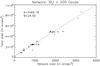 |
Fig. 5 Scatter plot between derived network area and the total area (on the image plane) of the 55 considered quiet-Sun magnetograms for a network threshold of |Bz|> 200 G. The dashed line shows the best linear fit (y = A + Bx) between the network area (x) and the total area (y). A similar linear monotonic dependence holds for the other two network thresholds (100 G, 300 G) considered in this analysis with respective linear fit coefficients (A,B) equal to (2177.41, 11.13) and (3288.36, 37.9). The linear fit coefficients (A,B) between network and total area measured on the heliographic plane for the network thresholds (100 G, 200 G, 300 G) are equal to (2337.97, 11.17), (3569.72, 23.95), and (3463.81, 38.73). |
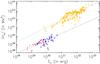 |
Fig. 6 Free magnetic energy – relative helicity diagram of solar quiet regions. Red/blue corresponds to negative/positive total magnetic helicity budgets, while asterisks denote regions centered within heliolatitudes of ±30° and diamonds denote regions centered on higher latitudes. The dashed line denotes the least-squares best fit of Eq. (3). Yellow asterisks show for comparison the free energy – relative helicity diagram of ARs derived by Tziotziou et al. (2012), while the dotted line shows the respective least-squares best fit. |
Figure 4 shows the derived free magnetic energy and relative magnetic helicity budgets of the 55 quiet-Sun regions as a function of the image plane magnetic network area, derived for the three considered threshold values. The higher the threshold value, the smaller the network area coverage as a percentage of the magnetogram area. As Fig. 4 suggests, there seems to be a monotonic dependence of free magnetic energy on the network area with a goodness r of the linear fit ranging between 0.71 and 0.76 depending on the threshold-dependent network mask. A similar monotonic relationship, although not as clear, seems to exist also between relative helicity and network area; the goodness-of-fit is low and ranges between 0.43 and 0.45. Derived fitting coefficients for the linear fits between helicity/energy and network area for all three different network thresholds are included in the plots of Fig. 4. The derived mean absolute deviation for helicity is 1.5 × 1039 Mx2, 1.49 × 1039 Mx2, and 1.5 × 1039 Mx2, respectively, for the used network thresholds of 100 G, 200 G, and 300 G, while for the energy the respective values are 3.14 × 1029 erg, 2.79 × 1029 erg, and 2.76 × 1029 erg. These values are one order of magnitude higher than the respective mean uncertainties of the relative helicity and free magnetic energy.
The monotonic dependence of helicity/energy to network area stems from the hierarchical structure of the magnetic field in quiet-Sun regions that concentrates at the boundaries of supergranular cells. Supergranular cells tend to have rather similar physical characteristics in terms of sizes and magnetic flux concentrations. As a consequence, a) derived helicity and energy budgets roughly depend on the number of supergranular cells present within the area under investigation, and b) the larger the area, the more supergranular cells are present, and hence the larger the derived network areas. Figure 5 clearly demonstrates a linear monotonic dependence between network area and the total area of the quiet-Sun magnetograms.
The network area seems to range from 10% (maximum phase) to 25% (minimum phase) of the solar disk area during a solar cycle (Fig. 3 in Caccin et al. 1998). Hence, we can derive the instantaneous budgets of free magnetic energy and relative helicity that are present globally in the quiet Sun during the minimum and maximum of the solar cycle using the linear relations shown in Fig. 4, and assuming that the aforementioned network area variance with solar cycle also holds for the other invisible half of the solar disk. Since we are dealing with image plane areas, the solar disk is considered to be a circle; all area-integrated results therefore, if areas on the heliographic plane were considered instead (whole Sun viewed as a sphere), would be larger by almost a factor of two. Derived values are presented in Table 1. The instantaneous global budgets of energy for the quiet Sun are similar to the respective budgets of a sizeable AR that is able to produce an eruptive X-class flare. The amplitude of helicity lags behind because of the incoherent helicity sense, resulting in the absence of a dominant helicity sign and hence in even lower net (algebraic) helicities.
3.3. Energy-helicity diagram of quiet-Sun regions
With the derived instantaneous free magnetic energy and relative magnetic helicity budgets of the selected 55 vector magnetograms we constructed the first free-energy – relative helicity diagram (hereafter energy – helicity [EH] diagram) of solar quiet regions. This diagram is shown in Fig. 6; the respective EH diagram of ARs derived by Tziotziou et al. (2012) is also shown in the same figure for comparison.
Both relative-helicity and free magnetic-energy budgets are much lower in quiet-Sun regions than in ARs. This stems from a) the much lower magnetic fluxes present in quiet-Sun regions than in ARs, b) the lower amount of free magnetic energy available in quiet-Sun regions because they are closer to a potential configuration than ARs, and c) the absence of a dominant net helicity in quiet-Sun regions in contrast to ARs. As already discussed in Sect. 3.1, the ratio Hpos/|Hneg| between the positive (Hpos) and the negative (Hneg) helicity components of the net helicity Hm, shows a clear incoherence (lack of preference) in helicity sign for quiet-Sun regions.
The EH diagram of Fig. 6 shows, like in ARs, a
nearly monotonic dependence between Ec and Hm in quiet-Sun
regions. However, in contrast to ARs, this dependence is the result of the presence of
hierarchical structures in the network area, as previously discussed in Sect. 3.2, and the monotonic dependence of both free magnetic
energy and relative magnetic helicity on the network and total area (Figs. 4 and 5). This
monotonic relation seems to be a logarithmic scaling of the form  (3)between
absolute relative helicity and free magnetic energy. We also note that the EH diagram
shows an appreciable segregation between positive-helicity and negative-helicity-dominated
regions, with the former being on the higher end of the EH diagram. Moreover, the only
quiet-Sun region showing a net helicity budget (see Sect. 3.1) also follows the derived linear monotonic relation. This region possesses
both the lowest helicity and energy budgets and is not presented in the EH diagram because
they are both almost two orders of magnitude lower than its lower end.
(3)between
absolute relative helicity and free magnetic energy. We also note that the EH diagram
shows an appreciable segregation between positive-helicity and negative-helicity-dominated
regions, with the former being on the higher end of the EH diagram. Moreover, the only
quiet-Sun region showing a net helicity budget (see Sect. 3.1) also follows the derived linear monotonic relation. This region possesses
both the lowest helicity and energy budgets and is not presented in the EH diagram because
they are both almost two orders of magnitude lower than its lower end.
The derived index of 0.815 of the monotonic relation between free magnetic energy and relative helicity in quiet-Sun regions is very close to the respective index of 0.897 for ARs (Tziotziou et al. 2012), as Fig. 6 shows. This suggests that if quiet-Sun regions had a predominant sign of helicity sign, like in ARs, their EH diagram would be a nearly continuous extension of the respective diagram for ARs toward lower values. This is fairly well seen with free magnetic energies alone, but helicity extension toward lower values is discontinuous because of the incoherence in helicity sign for quiet-Sun regions.
4. Discussion and conclusions
We have applied the recently proposed NLFF field method by Georgoulis et al. (2012) to calculate the instantaneous free magnetic energy and relative magnetic helicity budgets of quiet-Sun regions from single photospheric vector magnetograms. On a sample of 55 such magnetograms we found (1) a nearly monotonic relation between free-magnetic-energy/relative-helicity and magnetic network area (Fig. 4) as well as total area (Fig. 5), and as a consequence, (2) a nearly monotonic relation between the free magnetic energy and the relative magnetic helicity in quiet-Sun regions (Fig. 6). Derived energy/helicity budgets are much lower than the respective budgets of ARs reported by Tziotziou et al. (2012).
Free magnetic energy budgets of quiet-Sun regions represent a rather continuous extension of respective AR budgets towards lower values (Fig. 6). On the other hand, the corresponding helicity transition is discontinuous due to the lack of a dominant sense of relative magnetic helicity in quiet-Sun regions in contrast to ARs (Tziotziou et al. 2012, 2013). However, globally quiet-Sun regions show instantaneous budgets of free energy and, to a lesser extent, relative helicity that are similar to those of a sizable AR. Furthermore, they do not show any hemispheric helicity preference, contrary to previous reports (e.g. Georgoulis et al. 2009), but this might well be a selection effect, since most of the analyzed quiet-Sun areas cover parts of both north and south hemispheres.
The derived monotonic relations between the instantaneous budgets of energy/helicity and magnetic network area can be used to infer the respective budgets for an entire solar cycle. For such a derivation the respective helicity/energy injection rates have to be evaluated. Since magnetic flux concentrations used for the calculation of the instantaneous budgets are concentrated in supergranular boundaries (magnetic network), it can be assumed that the instantaneous budgets of energy/helicity replenish within the lifetime of supergranules, which is on the order of 1.8 ± 0.9 d (see Rieutord & Rincon 2010, and references therein). However, this assumption, although valid for the free magnetic energy that is always dissipated through resistive processes, such as reconnection, is not always valid for helicity. The latter, if not bodily removed, is roughly conserved during reconnection and can only be transferred to nearby regions via existing large-scale magnetic connections. Assuming that a) both quantities dissipate/replenish within the supergranular lifetime, and b) a sinusoidal variation of the network area between 10% and 25% within a solar cycle (see Fig. 3 in Caccin et al. 1998), we can derive the total quiet-Sun budgets for free magnetic energy and helicity in a solar cycle. The derived values for different network thresholds are presented in Table 2. The derived helicity budgets of ~1045 Mx2 are two orders of magnitude higher than the value of ~1043 Mx2 reported by Welsch & Longcope (2003) and an order of magnitude higher than the value of ~1.5 × 1044 Mx2 reported by Georgoulis et al. (2009). However, we must stress the high uncertainties attached to our solar-cycle helicity derivation, which mostly stem from the weakness of the used linear fit (Fig. 4) as expressed by the low values of the goodness r. Moreover, the estimates of Welsch & Longcope (2003) and Georgoulis et al. (2009) relied on typical photospheric flow velocities and the respective helicity injection rates. These have been found to underestimate the respective integrated budgets (Tziotziou et al. 2013).
This work presents the first inference of the quiet-Sun free-energy budget over an entire solar cycle. However, we do know that energy in the magnetic network is dissipated, mostly through reconnection, in fine-scale structures residing at the supergranular boundaries, such as mottles and spicules (Tsiropoula et al. 2012). Tsiropoula & Tziotziou (2004) have reported a value of at least 1.2 × 10⁵ erg cm-2 s-1 for the energy flux from mottles, while Moore et al. (2011) reported a value of 7 × 10⁵ erg cm-2 s-1 from spicules by including co-generated Alvén waves. Assuming again a sinusoidal variation of the network area between 10% and 25% within a solar cycle, we can integrate these values to derive respective energies within a solar cycle of 2 × 1035 erg and 1.2 × 1036 erg. These values are on the same order of magnitude as the derived values of free magnetic energy ~1036 erg (see Table 2). Hence, there seems to be enough free energy in the quiet Sun within a solar cycle to power fine-scale structures. Tsiropoula & Tziotziou (2004) have argued that considerable amounts of energy are also needed for heating the chromosphere. We note, however, that as discussed in Georgoulis et al. (2012), the derived free magnetic energy is a lower limit and hence there might be an even larger amount of free magnetic energy available in quiet-Sun regions.
Unfortunately, there exist no estimations of helicity in fine-scale structures, such as mottles and spicules, but these structures often show a helical behaviour (Jess et al. 2009; Curdt & Tian 2011; De Pontieu et al. 2012; Tsiropoula et al. 2012). Whether this behaviour is a manifestation of episodes of helicity removal and how this process actually takes place is still unknown. There exist, however, simulations of larger-scale solar polar jets (Pariat et al. 2009), observed in polar coronal holes, that investigate the reconnection-driven dynamics and the energy and helicity evolution. Future magneto-hydrodynamic simulations of fine-scale structures, combined with high-resolution observations of the chromosphere, are expected to shed light on the processes of heliospheric helicity expulsion – if any – from quiet-Sun regions.
Acknowledgments
Hinode is a Japanese mission developed and launched by ISAS/JAXA, with NAOJ as domestic partner and NASA and STFC (UK) as international partners and operated in co-operation with ESA and NSC (Norway). The Dutch Open Telescope is operated at the Spanish Observatorio del Roque de los Muchachos of the Instituto de Astrofísica de Canarias. This research has been carried out in the framework of the Research Projects hosted by the RCAAM of the Academy of Athens. This work was partially supported from the EU’s Seventh Framework Programme under grant agreement No. PIRG07-GA-2010-268245.
References
- Berger, M. A. 1984, Ph.D. Thesis, Cambridge, Harvard University [Google Scholar]
- Berger, M. A. 1999, Plasma Phys. Control. Fusion, 41, 167 [Google Scholar]
- Berger, M. A., & Field, G. B. 1984, J. Fluid Mech., 147, 133 [NASA ADS] [CrossRef] [Google Scholar]
- Caccin, B., Ermolli, I., Fofi, M., & Sambuco, A. M. 1998, Sol. Phys., 177, 295 [NASA ADS] [CrossRef] [Google Scholar]
- Chesny, D. L., Oluseyi, H. M., & Orange, N. B. 2013, ApJ, 778, L17 [NASA ADS] [CrossRef] [Google Scholar]
- Curdt, W., & Tian, H. 2011, A&A, 532, L9 [NASA ADS] [CrossRef] [EDP Sciences] [Google Scholar]
- Demoulin, P., Pariat, E., & Berger, M. A. 2006, Sol. Phys., 233, 3 [NASA ADS] [CrossRef] [Google Scholar]
- De Pontieu, B., Carlsson, M., Rouppe van der Voort, L. H. M., et al. 2012, ApJ, 752, L12 [NASA ADS] [CrossRef] [Google Scholar]
- DeVore, C. R. 2000, ApJ, 539, 944 [NASA ADS] [CrossRef] [Google Scholar]
- Finn, J. M., & Antonsen, T. M., Jr. 1985, Commun. Plasma Phys. Control. Fusion, 9, 111 [Google Scholar]
- Galsgaard, K., Parnell, C. E., & Blaizot, J. 2000, A&A, 362, 395 [NASA ADS] [Google Scholar]
- Gary, G. A., & Hagyard, M. J. 1990, Sol. Phys., 126, 21 [NASA ADS] [CrossRef] [Google Scholar]
- Georgoulis, M. K. 2005, ApJ, 629, L69 [NASA ADS] [CrossRef] [Google Scholar]
- Georgoulis, M. K., & Rust, D. M. 2007, ApJ, 661, L109 [NASA ADS] [CrossRef] [Google Scholar]
- Georgoulis, M. K., Rust, D. M., Pevtsov, A. A., Bernasconi, P. N., & Kuzanyan, K. M. 2009, ApJ, 705, L48 [NASA ADS] [CrossRef] [Google Scholar]
- Georgoulis, M. K., Tziotziou, K., & Raouafi, N.-E. 2012, ApJ, 759, 1 [NASA ADS] [CrossRef] [Google Scholar]
- Hagenaar, H. J., Schrijver, C. J., & Title, A. M. 1997, ApJ, 481, 988 [NASA ADS] [CrossRef] [Google Scholar]
- Jess, D. B., Mathioudakis, M., Erdélyi, R., et al. 2009, Science, 323, 1582 [NASA ADS] [CrossRef] [PubMed] [Google Scholar]
- Kontogiannis, I., Tsiropoula, G., Tziotziou, K., & Georgoulis, M. K. 2010, A&A, 524, A12 [NASA ADS] [CrossRef] [EDP Sciences] [Google Scholar]
- Kontogiannis, I., Tsiropoula, G., & Tziotziou, K. 2011, A&A, 531, A66 [NASA ADS] [CrossRef] [EDP Sciences] [Google Scholar]
- Leka, K. D., Canfield, R. C., McClymont, A. N., & van Driel-Gesztelyi, L. 1996, ApJ, 462, 547 [NASA ADS] [CrossRef] [Google Scholar]
- Lites, B. W., Kubo, M., Socas-Navarro, H., et al. 2008, ApJ, 672, 1237 [NASA ADS] [CrossRef] [Google Scholar]
- Liu, S., Zhang, H. Q., & Su, J. T. 2011, Sol. Phys., 270, 89 [NASA ADS] [CrossRef] [Google Scholar]
- Low, B. C. 1994, Phys. Plasmas, 1, 1684 [NASA ADS] [CrossRef] [Google Scholar]
- Metcalf, T. R., Leka, K. D., Barnes, G., et al. 2006, Sol. Phys., 237, 267 [Google Scholar]
- Metcalf, T. R., De Rosa, M. L., Schrijver, C. J., et al. 2008, Sol. Phys., 247, 269 [Google Scholar]
- Meyer, K. A., Sabol, J., Mackay, D. H., & van Ballegooijen, A. A. 2013, ApJ, 770, L18 [NASA ADS] [CrossRef] [Google Scholar]
- Moore, R. L., Sterling, A. C., Cirtain, J. W., & Falconer, D. A. 2011, ApJ, 731, L18 [NASA ADS] [CrossRef] [Google Scholar]
- Pariat, E., Antiochos, S. K., & DeVore, C. R. 2009, ApJ, 691, 61 [NASA ADS] [CrossRef] [Google Scholar]
- Parnell, C. E. 2001, Sol. Phys., 200, 23 [NASA ADS] [CrossRef] [Google Scholar]
- Rieutord, M., & Rincon, F. 2010, Liv. Rev. Sol. Phys., 7, 2 [Google Scholar]
- Schrijver, C. J., & Harvey, K. L. 1994, Sol. Phys., 150, 1 [NASA ADS] [CrossRef] [Google Scholar]
- Schrijver, C. J., Title, A. M., van Ballegooijen, A. A., Hagenaar, H. J., & Shine, R. A. 1997, ApJ, 487, 424 [NASA ADS] [CrossRef] [Google Scholar]
- Schrijver, C. J., De Rosa, M. L., Metcalf, T. R., et al. 2006, Sol. Phys., 235, 161 [Google Scholar]
- Tsiropoula, G., & Tziotziou, K. 2004, A&A, 424, 279 [NASA ADS] [CrossRef] [EDP Sciences] [Google Scholar]
- Tsiropoula, G., Tziotziou, K., Kontogiannis, I., et al. 2012, Space Sci. Rev., 169, 181 [NASA ADS] [CrossRef] [Google Scholar]
- Tziotziou, K., Georgoulis, M. K., & Raouafi, N.-E. 2012, ApJ, 759, L4 [NASA ADS] [CrossRef] [Google Scholar]
- Tziotziou, K., Georgoulis, M. K., & Liu, Y. 2013, ApJ, 772, 115 [NASA ADS] [CrossRef] [Google Scholar]
- Uritsky, V. M., Davila, J. M., Ofman, L., & Coyner, A. J. 2013, ApJ, 769, 62 [Google Scholar]
- Wang, H., Tang, F., Zirin, H., & Wang, J. 1996, Sol. Phys., 165, 223 [NASA ADS] [CrossRef] [Google Scholar]
- Welsch, B. T., & Longcope, D. W. 2003, ApJ, 588, 620 [NASA ADS] [CrossRef] [Google Scholar]
- Welsch, B. T., Abbett, W. P., De Rosa, M. L., et al. 2007, ApJ, 670, 1434 [NASA ADS] [CrossRef] [Google Scholar]
- Wiegelmann, T., Solanki, S. K., Borrero, J. M., et al. 2013, Sol. Phys., 283, 253 [Google Scholar]
- Woodard, M. F., & Chae, J. 1999, Sol. Phys., 184, 239 [NASA ADS] [CrossRef] [Google Scholar]
- Zhao, M., Wang, J.-X., Jin, C.-L., & Zhou, G.-P. 2009, Res. Astron. Astrophys., 9, 933 [NASA ADS] [CrossRef] [Google Scholar]
- Zirin, H., & Wang, H. 1993, Nature, 363, 426 [NASA ADS] [CrossRef] [Google Scholar]
All Tables
All Figures
|
Fig. 1 Central heliographic positions for the 55 vector quiet-Sun magnetograms included in our analysis. The size of the diamonds implies normalized (to the maximum value) area size. Red/blue diamonds correspond to negative/positive total magnetic helicity budgets (see Sect. 3.1). |
| In the text | |
|
Fig. 2 Top panel: an observed SOT/SP magnetogram (vertical field component Bz) of a quiet-Sun region studied here. White/black denotes positive/negative magnetic field concentrations. Bottom panel: inferred magnetic connectivity of the region, showing the vertical magnetic field component in grayscale with the contours bounding the identified magnetic partitions. The flux-tube connections identified by the magnetic connectivity matrix are represented by line segments connecting the flux-weighted centroids of the respective pair of partitions. Red, blue, yellow, and cyan segments denote magnetic flux contents within the ranges [1016, 1017] Mx, [1017, 1018] Mx, [1018, 1019] Mx, and >1019 Mx, respectively. Only connections closing within the field-of-view are shown. |
| In the text | |
|
Fig. 3 Left panel: an Hα image observed with the Dutch Open Telescope (see Kontogiannis et al. 2010, for details). Middle panel: corresponding SOT/SP magnetogram (vertical field component Bz) of the quiet-Sun region with the inferred connectivity overlaid (see caption of Fig. 2 for an explanation of the magnetic connectivity matrix). Right panel: field lines of the potential field extrapolation of Kontogiannis et al. (2010, their Fig. 2) overlaid on the Hα image of the left panel. |
| In the text | |
|
Fig. 4 Derived free magnetic energy (left column) and relative magnetic helicity (right column) budgets as a function of the image plane magnetic network area for three different network area thresholds of 100 G, 200 G, and 300 G. In plots involving helicity budgets, red/blue colors correspond to negative/positive magnetic-helicity budgets. Quiet-Sun regions centered within latitudes of ±30° (see Fig. 1) are represented by asterisks, while regions centered on larger latitudes are presented by diamonds. Error bars in helicity are also shown, while respective energy errors are not indicated because of their very small amplitude (~1028 erg). Dashed lines show the best linear fit between helicity/energy and network area (y = A + Bx, where y represents helicity/energy and x the network area). Derived fitting coefficients A and B, the goodness of the fit r, as well as the mean network area as a percentage of the magnetogram area are also registered within each plot. Derived linear fit coefficients (A,B) between free magnetic energy and heliographic plane network area are equal to (−2.89 × 1029, 4.33 × 1026), (− 2.53 × 1029, 9.39 × 1026), and (−2.21 × 1029, 1.42 × 1027) for the three network thresholds, while for relative magnetic helicity and heliographic plane network area they are equal to (−5.06 × 1037, 7.89 × 1035), (−5.63 × 1037, 2.31 × 1036), and (−6.53 × 1035, 3.54 × 1036). |
| In the text | |
|
Fig. 5 Scatter plot between derived network area and the total area (on the image plane) of the 55 considered quiet-Sun magnetograms for a network threshold of |Bz|> 200 G. The dashed line shows the best linear fit (y = A + Bx) between the network area (x) and the total area (y). A similar linear monotonic dependence holds for the other two network thresholds (100 G, 300 G) considered in this analysis with respective linear fit coefficients (A,B) equal to (2177.41, 11.13) and (3288.36, 37.9). The linear fit coefficients (A,B) between network and total area measured on the heliographic plane for the network thresholds (100 G, 200 G, 300 G) are equal to (2337.97, 11.17), (3569.72, 23.95), and (3463.81, 38.73). |
| In the text | |
|
Fig. 6 Free magnetic energy – relative helicity diagram of solar quiet regions. Red/blue corresponds to negative/positive total magnetic helicity budgets, while asterisks denote regions centered within heliolatitudes of ±30° and diamonds denote regions centered on higher latitudes. The dashed line denotes the least-squares best fit of Eq. (3). Yellow asterisks show for comparison the free energy – relative helicity diagram of ARs derived by Tziotziou et al. (2012), while the dotted line shows the respective least-squares best fit. |
| In the text | |
Current usage metrics show cumulative count of Article Views (full-text article views including HTML views, PDF and ePub downloads, according to the available data) and Abstracts Views on Vision4Press platform.
Data correspond to usage on the plateform after 2015. The current usage metrics is available 48-96 hours after online publication and is updated daily on week days.
Initial download of the metrics may take a while.