| Issue |
A&A
Volume 563, March 2014
|
|
|---|---|---|
| Article Number | A4 | |
| Number of page(s) | 5 | |
| Section | Planets and planetary systems | |
| DOI | https://doi.org/10.1051/0004-6361/201323300 | |
| Published online | 26 February 2014 | |
Research Note
New determination of the HCN profile in the stratosphere of Neptune from millimeter-wave spectroscopy
1
Max-Planck-Institut für Sonnensystemforschung,
Justus-von-Liebig-Weg 3,
37077
Göttingen,
Germany
e-mail:
This email address is being protected from spambots. You need JavaScript enabled to view it.
2
Department of Astrophysical Sciences, Princeton
University, Princeton
NJ
08544,
USA
3
Univ. Bordeaux, LAB, UMR 5804, 33270
Floirac,
France
4
CNRS, LAB, UMR 5804, 32270
Floirac,
France
Received: 20 December 2013
Accepted: 31 January 2014
Abstract
Context. Periodic monitoring of the atmospheric composition is the cornerstone of planetary atmospheric science. It reveals temporal and/or spatial variations. Ground-based observations of rotational lines from the (sub-)millimeter wavelength range is a suitable method to obtain the mean HCN profile in Neptune’s startosphere.
Aims. We aimed at deriving new constraints on the disk-averaged HCN stratospheric profile and abundance. The 14-year gap between the last published observations and ours of HCN in Neptune can be used to constrain any possible time variation of this main nitrogen-bearing molecule at the probed altitudes. This temporal variation could additionally reveal, albeit indirectly, the dominant process responsible for the origin of the nitrogen compoundsin the stratosphere of Neptune.
Methods. Spectra of the HCN (J = 3–2) line at 265.886 GHz were obtained with the 1.3 mm receiver of the Submillimeter Telescope (SMT) at the Arizona Radio Observatory (ARO) using several backends simultaneously. The spectral resolution of the analyzed datasets was 1 MHz and 250 kHz, providing a signal-to-noise ratio of 20 and 11, respectively. Pre-processing of the spectra involved baseline removal and de-noising using the empirical mode decomposition technique. The spectra were then inverted using a line-by-line radiative transfer model to obtain the vertical profile of HCN between 2 mbar to 10 μbar and derive the column density.
Results. The retrieved mean stratospheric HCN mole fraction is (1.3 ± 0.6) × 10-9 above 0.5 millibar, corresponding to a column density of 2.2 × 10¹⁴ molecules cm-2. The data are consistent with a pronounced HCN decrease below the 0.6 mbar level, which agrees with previous findings.
Key words: submillimeter: planetary systems / planets and satellites: atmospheres / planets and satellites: composition
© ESO, 2014
1. Introduction
Neptune is the most distant planet in the solar system, even though it most likely did not form at its current location (Levison & Stewart 2001; Gomes et al. 2004). To improve formation and evolution models, accurate knowledge of the composition of the planet atmosphere is required. Neptune is expected to show strong heavy element enrichment with respect to the protosolar value (e.g. Hersant et al. 2004). For instance, the strong enrichment in carbon and oxygen is reflected in the high abundances of CH4 (Baines et al. 1995) and CO (Marten et al. 1993; Lodders & Fegley 1994). However, despite Neptune’s strong internal heat source (Pearl & Conrath 1991) the upper tropospheric temperatures are low enough to prevent several species, such as H2O, from reaching observable altitudes. It was therefore a surprise when Marten et al. (1993) and Feuchtgruber et al. (1997) identified condensible species such as HCN, H2O, and CO2 in Neptune’s stratosphere. The first detection of HCN (along with CO) in the atmosphere of Neptune was obtained by Marten et al. (1993) with a mole fraction (1 ± 0.3) × 10-9 above its condensation level, while Rosenqvist et al. (1992) derived a value of (3 ± 1.5) × 10-10. Since transport of HCN from the deep atmosphere through the tropopause “cold trap” is unlikely, it must be either delivered through cometary impacts or be produced locally in the stratosphere through photochemical pathways, which in turn require availability of atomic nitrogen. Therefore, the explanation of the observed abundance of HCN and its vertical profile depends on the external/internal origin of the N atoms in the stratosphere. So far, the two scenarios investigated involve a transport of escaping N atoms from the moon Triton and/or a transport of N2 during upwelling events with subsequent photodissociation by the solar EUV photons or galactic cosmic rays. Lellouch et al. (1994) analyzed IRAM 30 m observations and inferred a stratospheric constant value of (3.2 ± 0.8) × 10-10 at 2 mbar and a sharp decrease at the condensation level. Using detailed photochemical modeling, they concluded that both internal and external sources of nitrogen are viable. To better constrain the HCN vertical profile, Marten et al. (2005) performed new observations of Neptune in 1998 and simultaneously derived HCN and the temperature profile from a CO line. These results were consistent with the HCN mole fraction measured back in 1991, but the vertical profile showed a pronounced undersaturation starting as high as 0.2 mbar.
Other possible exogenic sources of nitrogen for Neptune must also be considered: 1) interplanetary dust particles (Landgraf et al. 2002), which result from comet activity and asteroid collision; and 2) large-comet impacts (Lellouch et al. 1995). For CO, for instance, the comet source has been demonstrated in Jupiter (Bézard et al. 2002), and proposed for CO in Saturn (Cavalié et al. 2010) and Neptune (Lellouch et al. 2005), while the situation remains unclear at Uranus (Cavalié et al. 2014).
In the present work, we aim to retrieve new constraints on the HCN vertical profile from high signal-to-noise ratio (S/N) observations. A second goal is to determine whether there has been any temporal variability of HCN since it was last observed in 1998 (Marten et al. 2005). Most sources of atomic nitrogen in the stratosphere can be subject to variability associated with 1) dynamical perturbation from the deep interior (Orton et al. 2007); or 2) the geologic/volcanic activity on Triton (Brown et al. 1990; Grundy et al. 2010); and 3) the vertical and horizontal mixing after a comet impact (e.g., Cavalié et al. 2013, in Jupiter). Such events might be reflected in the vertical profile of HCN or in its mean stratospheric abundance.
The paper is structured as follows: Sect. 2 focuses on the observations. Section 3 gives a description of the forward model and presents the data analysis. Section 4 details the inversion approach and provides a full error analysis. Results are summarized and discussed in Sect. 5.
2. Observations
The HCN (J = 3–2) rotational transition at 265.886 GHz was observed in Neptune using the 10 m Submillimeter Telescope (SMT; Baars & Martin 1996; Baars et al. 1999) located at the Mount Graham International Observatory. The observations were performed with the 1.3 mm sideband separating superconductor-insulator-superconductor (SIS) receiver. This receiver enabled us to observe horizontal vertical polarizations simultaneously and to improve the S/N by averaging both polarizations. We used the Forbes filterbanks (F1M and FQM) with resolutions of 1 MHz and 250 kHz, the chirp transform spectrometer (CTSB) with a resolution of 40 kHz (Hartogh & Hartman 1990), and the acousto-optical spectrometers (AOSA, AOSB and AOSC) with resolutions of 934, 913, and 250 kHz, respectively.
The observations were carried out on 12–13 and 28–29 April 2012 with generally good observing conditions (τ ≈ 0.2). The angular diameter of Neptune was 2.3 arcsec, and the subobserver latitude was ≈28°S. First, the standard position-switching observing mode was used, and a reference sky position separated from Neptune by 0.5′ was observed for the same amount of time and subtracted from the onsource observations for the first 10 scans on 12 April. The dual beam-switching observing mode was used thereafter. We used 8-min scans in both observing modes. The average system temperature of the receiver was 320 K with ~15% fluctuations during the observing period; the total observing time was 22.5 h.
The HCN (J = 3–2) raw spectra obtained with the Forbes filterbank at 1 MHz resolution are shown in Fig. 1. Individual exposures were co-added according to statistical weights proportional to the inverse square of the system temperature.
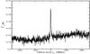 |
Fig. 1 Antenna temperature spectra of the HCN (J = 3–2) at 265.886 GHz on Neptune at a resolution of 1 MHz. |
A weak baseline ripple was present in the measured data and was removed as part of the post-processing routine. For this purpose we used the empirical mode decomposition (EMD) procedure (Huang et al. 1998; Battista et al. 2007) that decomposes the original signal into all oscillatory modes captured in the signal, the so-called intrinsic mode functions (IMF). These include the highest frequency, (noise), as well as the lowest, (baseline), components. The IMFs have two convenient properties: 1) the IMFs are additive; and 2) no information is lost in the process of extracting them. Hence, we can simply subtract the baseline ripple from the data as well as the highest frequency IMF that is generally associated with the random noise component (more discussion in de Val-Borro et al. 2012). The root-mean-square (rms) of the de-noised 1 MHz spectra is about 30% lower, which yields a final S/N of about 20.
3. Data analysis
Forward model
We used a line-by-line code (Jarchow & Hartogh 1995), that has previously been used for the analysis of the Herschel/HIFI observations (Hartogh et al. 2010a,b) as well as ground-based observations (Rengel et al. 2008a,b). A spherical geometry was assumed and limb emissions were included. The smearing effect caused by the 16-hour planet rotation was taken into account. The HCN collisional half-width coefficients with H2 and He come from the data in Table III of Rohart et al. (1987). The collision-induced absorption by H2–H2, H2–He, and H2–CH4, which dominates the continuum opacity was calculated with the model of Borysow et al. (1985, 1988), and Borysow & Frommhold (1986). The individual opacity sources were assumed to have a constant profile with H2 and He volume mixing ratios (quoted with uncertainty) of 83.1 % and 14.9
 % (Burgdorf et al. 2003), respectively. The CH4 is not entirely trapped below the tropopause. Sporadic upwelling events allow CH4 to penetrate into the stratosphere at the south pole. The estimates from disk-averaged measurements range between ≈0.13–0.8% (Lunine 1993; Orton et al. 2007). The most recent results of the Herschel/PACS data analysis are consistent with a stratospheric volume mixing ratio of CH4 at 0.15 ± 0.02% (Lellouch et al. 2010). A constant CH4 volume mixing ratio of 2% was taken for p > 1.5 bar (Lindal 1992; Baines et al. 1995).
The disk-averaged kinetic temperature profile in the stratosphere of Neptune is not known precisely and the reported variations probably reflect meteorological processes that skew the disk-averaged estimates. Several published profiles are shown in Fig. 2. In this work the profile based on Feuchtgruber et al. (2013) was used, which is very similar to that derived by Marten et al. (2005) (up to 0.6 mbar) from inversion of the CO spectra. The data on HCN line strength were taken from the JPL Molecular Spectroscopy catalogue (Pickett et al. 1998). The line shape was modeled with the Voigt function.
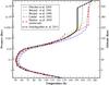 |
Fig. 2 Disk-averaged kinetic temperature profiles obtained from several different observations during the past 20 years. The largest differences are on the order of 5 K around tropopause, but increase to more than 15 K at 1 mbar. The temperature profile retrieved by Marten et al. (2005) is shown in red. In our analysis, we use the profile from Feuchtgruber et al. (2013) plotted with a thick black line with squares. |
Retrieval approach
The HCN (J = 3–2) line is optically thin, with optical depth at line center 0.12 for a nadir geometry, but becomes moderately optically thick (<10) for limb rays. The vertical extent across which we can obtain information on the HCN is governed by the so-called Jacobians (Rodgers 2000), defined as a derivative of intensity with respect to the mole fraction. These are shown in Fig. 3 at several frequency offsets from the line center as a function of pressure level and height above the 1-bar level. It should be noted that these are disk-averaged, hence truly reflecting the vertical extent of sensitivity of the observations to the HCN mole fraction. The line center shows sensitivity extending up to 350 km, but the vertical resolution in general is rather poor, as demonstrated by the strongly overlapping peaks. The HCN profile was set to zero below its condensation level (110 km, 3 mbar), which is the lowest level of sensitivity to HCN. The radiances coming from below this level are dominated by the continuum, and for this reason the Jacobians are not displayed for the entire pressure range in Fig. 3.
Our retrieval approach relies on a full parameter search that minimizes the χ2 of differences between measured and calculated radiances for a total of 40 000 profiles. The HCN vertical distribution is assumed to take a form q(z) = 0.5A1 × (1 + tanh [(z − A2)/(2A3)]), where A1 controls the constant mole fraction above the condensation level, A2 is the height where it starts decreasing, and A3 is the parameter describing the slope of decay below the level described by A2. This parametrization captures the physics of the HCN profile well and requires only three parameters to be retrieved.
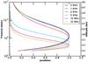 |
Fig. 3 Disk-averaged Jacobians for various frequency offsets with regard to the HCN line center assuming a 1 × 10⁻⁹ constant HCN mole fraction above the condensation level (3 mbar). The curves are normalized to the highest value. The rotational smearing leads to much narrower peaks that reach maximum at ≈175 km for the line center frequency. Pure pencil-beam Jacobians for the nadir geometry at the line center peak at around 250 km (not shown). |
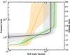 |
Fig. 4 HCN mole fraction profile obtained with the best fit to the data (thick black line). Other possible profiles fitting the data based on the χ2 within 1σ noise are shown as the shaded (dark gray) envelope, and the total 1σ uncertainty plotted in light gray. For comparison, we show the profiles of Lellouch et al. (1994) (thick orange) and Marten et al. (2005) (thick green) along with their estimated uncertainties (shaded regions of the respective colors). |
4. Results
4.1. Retrieval results
The best fit was obtained for the following HCN profile parameters: A1 = 1.32 × 10⁻⁹, A2 = 174 km (0.5 mbar), and A3 = 5 km. The best-fit profile (black line) and associated 1σ noise uncertainty (dark-gray shading) and 1σ total uncertainty (light-gray shading) are shown in Fig. 4. The comparison of the best-fit model with the measurement (along with 1σ noise) are presented in Fig. 5. The retrieved HCN mole fraction shows a pronounced undersaturation in the stratosphere starting at about 0.5 mbar, well above the condensation level, and the stratospheric nominal value is consistent with that of obtained by Marten et al. (2005). The corresponding column density is (2.2 ±0.1) × 1014 molecules cm-2. It should be kept in mind that no condensation level was specified a priori, as done by other investigators, and we show only profiles derived with our three-parameter description of the HCN profile. The information on the HCN profile below the 1-mbar level comes from the line wings (| f − f0| > 15 MHz), where the S/N approaches 1, and hence this information is poorly constrained by the measurement. Below this region, the profile could slowly join the condensation level without significantly changing the fit.
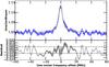 |
Fig. 5 Top panel: measured radiance as the line-to-continuum ratio with 1σ noise error bars (blue) and the radiances calculated for the acceptable solutions for the three-parameter HCN profile. The bottom panel show the residual (measured – synthetic) radiances, and the dashed horizontal lines are the 1σ limits of measurement noise. |
Best-fit values and associated 1σ uncertainties.
4.2. Error analysis
The total uncertainty in the retrieved parameters has both random and systematic components, where the latter are dominant for these observations. The random uncertainty component stems primarily from the thermal noise. The systematic uncertainty sources are 1) the spectral line parameters, including the collisional half-width; 2) the thermal and pressure profiles; and 3) data calibration. The uncertainty in the retrieved HCN profile is estimated by varying a given parameter within its range of uncertainty and again retrieving the three parameters.
The HCN (J = 3–2) line strength has an estimated uncertainty of 5% (difference between HITRAN, GEISA, and JPL line catalogs), which results in a negligible difference in the line amplitude modeling. However, the pressure broadening half-width parameters for H2 and He are accurate only to within ~40% (Rohart et al. 1987) and this strongly impacts the line profile. The variability of temperature profiles in the stratosphere (Fig. 2) has a negligible effect on the retrieved HCN profile. The tropopause value of temperature/pressure can influence the line/continuum ratio through hydrostatic effects. We took the most different temperature profile (that of Fletcher et al. (2010)), and repeated our retrieval to infer the related uncertainty. Finally, a conservative data calibration error of 10% was assumed, which includes the continuum calibration. Our baseline ripple removal procedure has no significant effect on the final calibration uncertainty.
5. Summary and discussion
New observations of HCN emission from the stratosphere of Neptune were obtained with the SMT in April 2012, nearly 14 years after the last reported observations of Marten et al. (2005). These measurements were used to retrieve the HCN vertical profile, specifically, the stratospheric mole fraction and the altitude below which the profile starts to decrease. The mean stratospheric HCN mole fraction is consistent with that obtained by Marten et al. (2005), confirming that the values derived by Rosenqvist et al. (1992) and Lellouch et al. (1994) were about a factor of 3 too low. The main result is the confirmation that the HCN profile sharply decreases below the 0.5 mbar level, that is, well above the condensation level.
The next step to take is to reproduce the main vertical profile features retrieved from observations with a photochemical model (Dobrijevic et al. 2010; Hébrard et al. 2012) to test various possible sources for N. In addition, mapping the HCN emission across Neptune may reveal an inhomogeneous distribution of HCN, which might result from a recent comet impact (e.g. Cavalié et al. 2013, for H2O in Jupiter’s stratosphere) or from a local source, for instance, Triton (e.g., Hartogh et al. 2011, for Saturn).
The HCN observations do not reveal any significant temporal variability since the 1998 observations of Marten et al. (2005). However, given the long orbital period of Neptune (165 years), a periodic monitoring remains highly desirable in the future, because it might unveil long-term seasonal variations or long-term aftermaths of a comet impact.
Acknowledgments
L.R. acknowledges support from the Special Priority Program 1488 (PlanetMag, http://www.planetmag.de) of the German Science Foundation. Results presented in this paper are based on observations obtained at the SMT, which is operated by the Arizona Radio Observatory (ARO), Steward Observatory, University of Arizona. We thank the ARO staff for their expertise and support during these observations. We thank B. Bézard for helpful comments and suggestions that improved the manuscript.
References
- Baars, J. W. M., & Martin, R. N. 1996, Rev. Mod. Astron. 9, 111 [NASA ADS] [Google Scholar]
- Baars, J. W. M., Martin, R. N., Mangum, J. G., McMullin, J. P., & Peters, W. L. 1999, PASP, 111, 627 [NASA ADS] [CrossRef] [Google Scholar]
- Baines, K. H., Mickelson, M. E., Larson, L. E., & Ferguson, D. W. 1995, Icarus, 114, 328 [NASA ADS] [CrossRef] [Google Scholar]
- Battista, B. M., Knapp, C., McGee, T., & Goebel, V. 2007, Society of Exploration Geophysicists, 72, 29 [Google Scholar]
- Bézard, B., Romani, P. N., Conrath, B. J., & Maguire, W. C. 1991, J. Geophys. Res., 96, 18961 [NASA ADS] [CrossRef] [Google Scholar]
- Bézard, B., Lellouch, E., Strobel, D., Maillard, J.-P., & Drossart, P. 2002, Icarus, 159, 95 [NASA ADS] [CrossRef] [Google Scholar]
- Borysow, A., & Frommhold, L. 1986, ApJ, 304, 849 [NASA ADS] [CrossRef] [Google Scholar]
- Borysow, J., Trafton, L., Frommhold, L., & Birnbaum, G. 1985, ApJ, 296, 644 [NASA ADS] [CrossRef] [Google Scholar]
- Borysow, J., Frommhold, L., & Birnbaum, G. 1988, ApJ, 326, 509 [NASA ADS] [CrossRef] [Google Scholar]
- Brown, R. H., Johnson, T. V., Kirk, R. L., & Soderblom, L. A. 1990, Science, 250, 431 [NASA ADS] [CrossRef] [Google Scholar]
- Burgdorf, M., Orton, G. S., Davis, G. R., et al. 2003, Icarus, 164, 244 [NASA ADS] [CrossRef] [Google Scholar]
- Cavalié, T., Hartogh, P., Billebaud, F., et al. 2010, A&A, 510, A88 [NASA ADS] [CrossRef] [EDP Sciences] [Google Scholar]
- Cavalié, T., Feuchtgruber, H., Lellouch, E., et al. 2013, A&A, 553, A21 [NASA ADS] [CrossRef] [EDP Sciences] [Google Scholar]
- Cavalié, T., Moreno, R., Lellouch, E., et al. 2014, A&A, 562, A33 [NASA ADS] [CrossRef] [EDP Sciences] [Google Scholar]
- de Val-Borro, M., Rezac, L., Hartogh, P., et al. 2012, A&A, 546, L4 [NASA ADS] [CrossRef] [EDP Sciences] [Google Scholar]
- Dobrijevic, M., Cavalie, T., Hebrard, E., et al. 2010, Planet. Space Sci., 58, 1555 [NASA ADS] [CrossRef] [Google Scholar]
- Feuchtgruber, H., Lellouch, E., de Graauw, T., et al. 1997, Nature, 389, 159 [NASA ADS] [CrossRef] [PubMed] [Google Scholar]
- Feuchtgruber, H., Lellouch, E., Orton, G., et al. 2013, A&A, 551, A126 [NASA ADS] [CrossRef] [EDP Sciences] [Google Scholar]
- Fletcher, L. N., Drossart, P., Burgdorf, M., Orton, G. S., & Encrenaz, T. 2010, A&A, 514, A17 [NASA ADS] [CrossRef] [EDP Sciences] [Google Scholar]
- Gomes, R. S., Morbidelli, A., & Levison, H. F. 2004, Icarus, 170, 492 [NASA ADS] [CrossRef] [Google Scholar]
- Grundy, W. M., Young, L. A., Stansberry, J. A., et al. 2010, Icarus, 205, 594 [NASA ADS] [CrossRef] [Google Scholar]
- Hartogh, P., & Hartman, G. K. 1990, Meas. Sci. Technol., 1, 592 [NASA ADS] [CrossRef] [Google Scholar]
- Hartogh, P., Blecka, M. I., Jarchow, C., et al. 2010a, A&A, 521, L48 [NASA ADS] [CrossRef] [EDP Sciences] [Google Scholar]
- Hartogh, P., Jarchow, C., Lellouch, E., et al. 2010b, A&A, 521, L49 [NASA ADS] [CrossRef] [EDP Sciences] [Google Scholar]
- Hartogh, P., Lellouch, E., Moreno, R., et al. 2011, A&A, 532, L2 [NASA ADS] [CrossRef] [EDP Sciences] [Google Scholar]
- Hébrard, E., Dobrijevic, M., Loison, J. C., Bergeat, A., & Hickson, K. M. 2012, A&A, 541, A21 [NASA ADS] [CrossRef] [EDP Sciences] [Google Scholar]
- Hersant, F., Gautier, D., & Lunine, J. I. 2004, Planet. Space Sci., 52, 623 [NASA ADS] [CrossRef] [Google Scholar]
- Huang, N. E., Shen, Z., Long, S., et al. 1998, Proc. Roy. Soc. London, 454, 903 [NASA ADS] [CrossRef] [Google Scholar]
- Jarchow, C., & Hartogh, P. 1995, in SPIE, 2586, 196 [Google Scholar]
- Landgraf, M., Liou, J.-C., Zook, H. A., & Grün, E. 2002, AJ, 123, 2857 [NASA ADS] [CrossRef] [Google Scholar]
- Lellouch, E., Romani, P. N., & Rosenquist, J. 1994, Icarus, 108, 112 [NASA ADS] [CrossRef] [Google Scholar]
- Lellouch, E., Paubert, G., Moreno, R., et al. 1995, Nature, 373, 592 [NASA ADS] [CrossRef] [PubMed] [Google Scholar]
- Lellouch, E., Moreno, R., & Paubert, G. 2005, A&A, 430, L37 [NASA ADS] [CrossRef] [EDP Sciences] [Google Scholar]
- Lellouch, E., Hartogh, P., Feuchtgruber, H., et al. 2010, A&A, 518, L152 [NASA ADS] [CrossRef] [EDP Sciences] [Google Scholar]
- Levison, H. F., & Stewart, G. R. 2001, Icarus, 153, 224 [NASA ADS] [CrossRef] [Google Scholar]
- Lindal, G. F. 1992, 103, 967 [Google Scholar]
- Lodders, K., & Fegley, Jr., B. 1994, Icarus, 112, 368 [NASA ADS] [CrossRef] [Google Scholar]
- Lunine, J. I. 1993, ARA&A, 31, 217 [NASA ADS] [CrossRef] [Google Scholar]
- Marten, A., Gautier, D., Owen, T., et al. 1993, ApJ, 406, 285 [NASA ADS] [CrossRef] [Google Scholar]
- Marten, A., Matthews, H. E., Owen, T., et al. 2005, A&A, 429, 1097 [NASA ADS] [CrossRef] [EDP Sciences] [Google Scholar]
- Orton, G. S., Encrenaz, T., Leyrat, C., Puetter, R., & Friedson, A. J. 2007, A&A, 473, L5 [NASA ADS] [CrossRef] [EDP Sciences] [Google Scholar]
- Pearl, J. C., & Conrath, B. J. 1991, J. Geophys. Res., 96, 18921 [Google Scholar]
- Pickett, H., Poynter, R., Cohen, E., et al. 1998, J. Quant. Spectr. Rad. Transf., 60, 883 [NASA ADS] [CrossRef] [Google Scholar]
- Rengel, M., Hartogh, P., & Jarchow, C. 2008a, Planet. Space Sci., 56, 1688 [NASA ADS] [CrossRef] [Google Scholar]
- Rengel, M., Hartogh, P., & Jarchow, C. 2008b, Planet. Space Sci., 56, 1368 [NASA ADS] [CrossRef] [Google Scholar]
- Rodgers, C. D. 2000, Inverse methods for Atmospheric Sounding: Theory and practice (World Scientific) [Google Scholar]
- Rohart, F., Derozier, D., & Legrand, J. 1987, J. Chem. Phys., 87, 5794 [NASA ADS] [CrossRef] [Google Scholar]
- Rosenqvist, J., Lellouch, E., Romani, P. N., Paubert, G., & Encrenaz, T. 1992, ApJ, 392, L99 [NASA ADS] [CrossRef] [Google Scholar]
All Tables
All Figures
|
Fig. 1 Antenna temperature spectra of the HCN (J = 3–2) at 265.886 GHz on Neptune at a resolution of 1 MHz. |
| In the text | |
|
Fig. 2 Disk-averaged kinetic temperature profiles obtained from several different observations during the past 20 years. The largest differences are on the order of 5 K around tropopause, but increase to more than 15 K at 1 mbar. The temperature profile retrieved by Marten et al. (2005) is shown in red. In our analysis, we use the profile from Feuchtgruber et al. (2013) plotted with a thick black line with squares. |
| In the text | |
|
Fig. 3 Disk-averaged Jacobians for various frequency offsets with regard to the HCN line center assuming a 1 × 10⁻⁹ constant HCN mole fraction above the condensation level (3 mbar). The curves are normalized to the highest value. The rotational smearing leads to much narrower peaks that reach maximum at ≈175 km for the line center frequency. Pure pencil-beam Jacobians for the nadir geometry at the line center peak at around 250 km (not shown). |
| In the text | |
|
Fig. 4 HCN mole fraction profile obtained with the best fit to the data (thick black line). Other possible profiles fitting the data based on the χ2 within 1σ noise are shown as the shaded (dark gray) envelope, and the total 1σ uncertainty plotted in light gray. For comparison, we show the profiles of Lellouch et al. (1994) (thick orange) and Marten et al. (2005) (thick green) along with their estimated uncertainties (shaded regions of the respective colors). |
| In the text | |
|
Fig. 5 Top panel: measured radiance as the line-to-continuum ratio with 1σ noise error bars (blue) and the radiances calculated for the acceptable solutions for the three-parameter HCN profile. The bottom panel show the residual (measured – synthetic) radiances, and the dashed horizontal lines are the 1σ limits of measurement noise. |
| In the text | |
Current usage metrics show cumulative count of Article Views (full-text article views including HTML views, PDF and ePub downloads, according to the available data) and Abstracts Views on Vision4Press platform.
Data correspond to usage on the plateform after 2015. The current usage metrics is available 48-96 hours after online publication and is updated daily on week days.
Initial download of the metrics may take a while.