| Issue |
A&A
Volume 563, March 2014
|
|
|---|---|---|
| Article Number | A138 | |
| Number of page(s) | 15 | |
| Section | Catalogs and data | |
| DOI | https://doi.org/10.1051/0004-6361/201322840 | |
| Published online | 25 March 2014 | |
Spectroscopic study of early-type multiple stellar systems
I. Orbits of spectroscopic binary subsystems⋆
Instituto de Ciencias Astronómicas, de la Tierra y del Espacio (ICATE-CONICET), Av. España 1512 sur, J5402DSP San Juan, Argentina
e-mail: This email address is being protected from spambots. You need JavaScript enabled to view it.
; This email address is being protected from spambots. You need JavaScript enabled to view it.
Received: 12 October 2013
Accepted: 26 November 2013
Abstract
Context. The present knowledge of stellar properties and dynamical structure of early-type multiple stellar systems is insufficient to offer useful statistical constraints for stellar formation models.
Aims. To increase the amount of observational information about the characteristics of early-type multiples, we carried out a spectroscopic monitoring to search for new spectroscopic components and to determine their orbits.
Methods. We observed 30 early-type multiple systems using the 2.15 m telescope and REOSC echelle spectrograph at the Complejo Astronómico El Leoncito (CASLEO) during 10 observing runs between 2008 and 2013. We measured radial velocities by cross-correlations and applied a spectral disentangling method to double-lined systems. We calculated orbital elements for the inner subsystem of each analysed multiple.
Results. In this first paper we present calculated orbits for six previously catalogued subsystems. Three subsystems had no previously published parameters, while we obtained more accurate orbits for the other three. In one case we found absolute masses and radii for the components by using available photometric data.
Conclusions. The long-term spectroscopic monitoring of multiple systems is a useful method of investigating the companions in intermediate hierarchical levels, particularly those that could affect the dynamical evolution of a close inner binary subsystem.
Key words: techniques: radial velocities / binaries: spectroscopic / stars: early-type / binaries: eclipsing / stars: chemically peculiar
Reduced spectra are only available at the CDS via anonymous ftp to cdsarc.u-strasbg.fr (130.79.128.5) or via http://cdsarc.u-strasbg.fr/viz-bin/qcat?J/A+A/563/A138
© ESO, 2014
1. Introduction
The frequency of binary and multiple (three or more components) systems is significant in all the stellar environments. Therefore, their statistical properties must be explained by models of stellar formation and evolution. The validity of such models can only be assessed by contrast with empirical results, provided that they are abundant and precise enough to adequately represent the population under study. In particular, multiple stellar systems are especially useful for contrasting such theories since they are characterized by a larger number of parameters than in binary stars. Many statistical relationships between such parameters can be compared with theoretical predictions thus providing important constraints for the models (Tokovinin 2008).
Most observational studies of multiples have focussed on searching for new components and analysing the properties of solar and late-type multiple systems (Duchêne & Bouvier 2008; Tokovinin 2004; Tokovinin et al. 2006). For solar-type stars, these have indicated that systems with multiplicity of order three or greater represents approximately 25% of the total of binary and multiple systems, while this fraction is 21% for low-mass stars (Duchêne & Kraus 2013). In these high-order systems, the period distribution of inner subsystems shows a maximum for periods between two and seven days and a marked decrease in the number of subsystems for longer periods (Tokovinin & Smekhov 2002; Tokovinin 2004). On the other hand, the searches for tertiary components of spectroscopic binary systems with solar-type components reveal that almost all binaries with periods of a few days are part of multiple systems (Tokovinin et al. 2006). This suggests that the presence of an outer companion plays an important role in the formation of tight pairs, presumably through energy and angular momentum exchanges (Duchêne & Kraus 2013).
Searches for spectroscopic binaries among A type stars have been carried out for several decades, while searches for low-mass visual companions for these objects have increased in recent years (Duchêne & Kraus 2013). The results of these studies led to a multiplicity frequency higher than 50% (including binaries). However, the available information is incomplete to carry out a reliable estimate of the frequency of systems with three or more components in this intermediate-mass range.
Currently it is accepted that most O and early-B type stars are part of binary and multiple systems. Even the isolated field massive stars would have belonged to multiple systems in the past and would have been expelled from them in supernova explosions or dynamical interactions (Sana & Evans 2011). On the other hand, the observational results suggest that multiplicity frequency is an increasing function of the stellar mass (Chini et al. 2013). They also indicate that for massive stars this frequency is greater in clusters and stellar associations than in the field and between runaway stars (Chini et al. 2012; Mason et al. 2009). Considering only confirmed companions, the multiplicity frequency among O-type stars is higher than 80% (Chini et al. 2012; Mason et al. 2009; Sana & Evans 2011). For early-B stars, a conservative lower limit of 60% could be adopted (Duchêne & Kraus 2013). However, these fractions do not distinguish between binary and multiple systems. At present, there are no specific estimations of the fraction of systems with three or more components among massive stars, whereas they do exist for low- and solar-mass stars. On the other hand, the studies of multiplicity in late-B stars are scarce and present very diverse results (Kouwenhoven et al. 2007; Chini et al. 2013; Schöller et al. 2010).
The last version1 of the Multiple Star Catalogue by Tokovinin (1997, hereafter MSC) contains 194 equatorial and southern (δ ≤ + 10°) multiple systems in which all components with catalogued spectral types are O, B, and A. Nonetheless, many of them lack detailed studies, and their multiplicity order can be expected to be higher than known. For that reason, there is a need to increase the current number of observational results on such systems.
We undertook an investigation with the aim of increasing the existing information about the multiplicity, stellar properties, and dynamical structure of early-type multiple systems. We focussed on collecting and analysing spectroscopic observations of catalogued multiple systems. As a result, we obtained orbits of catalogued subsystems and detected new binary and multiple subsystems. In this first paper, we describe the analysis and results for six multiples for which we have determined orbital parameters for the first time or have corrected their previously published orbits.
In Sect. 2 we comment on the general criteria for our target selection and describe the spectroscopic observations. Techniques of measuring radial velocities are described in Sect. 3. In Sect. 4 we present the results for the six systems studied in the present paper, while in Sect. 5 we discuss the hierarchical configuration of each system and the completeness of our survey. Finally, Sect. 6 summarizes our main conclusions.
2. Sample selection and observations
Our complete sample contains 30 multiple systems with δ ≤ + 10°, mostly triples, which belong to the field population of the Galaxy. We selected from the MSC multiples with components of spectral types O, B, and A, brighter than V = 10. This limiting magnitude was set in order to obtain, with our instrumentation, spectra with a signal-to-noise ratio high enough (S/N > 100) to detect eventual spectral morphological variations that indicate the presence of new components.
In particular, we selected systems with components classified as single stars without recent spectroscopic studies, as well as systems with components classified as spectroscopic or eclipsing binaries without computed orbits. In general, we did not observe components of visual pairs with separations between 1″ and 4″ owing to seeing limitations. Pairs with separations in this range usually cannot be observed separately without contamination from the companion, but neither are they close enough to ensure that both stars are included in the slit with the same light contribution in all the observations. Variations in the relative light contribution can introduce fake morphological changes or radial velocity variations. This limitation led us to exclude systems formed by visual pairs in this separation range where a wider additional component to be analysed does not exist.
With these constraints, we selected the systems listed in Table 1. All the basic data given in Table 1 have been extracted from MSC. The first column identifies the systems by its designation in the Washington Double Stars Catalogue (Mason et al. 2001, hereafter WDS). The second column lists the parallax. Columns 3 to 7 contain information on all the subsystems forming each multiple star: identification, type of subsystem, logarithm of the orbital period in days, separation between the components in arcseconds (or milliarcseconds indicated by “m”), and position angle. Finally, the last four columns contain visual magnitudes and spectral types for both components. For objects without spectral classification, the colour index (B − V) is listed, if available.
Data of the multiple systems analysed in this paper, obtained from the MSC.
The spectroscopic survey of the selected systems was carried out using the 2.15 m telescope and the REOSC echelle spectrograph at Complejo Astronómico El Leoncito (CASLEO), San Juan, Argentina. Most of the data (580 spectra) were obtained during 41 nights, spread over nine observing runs between February 2008 and November 2010. Some additional observations were carried out more recently during seven nights in February 2013. The spectra cover the wavelength range 3700−6300 Å with a resolution R = 13 300. Exposure times were calculated to achieve a signal-to-noise ratio S/N ~ 120, which requires, under good seeing conditions (~2.5″), an exposure time of 40 min for a star of magnitude V = 9.
Some components of the analysed systems are classified as spectroscopic binaries in MSC, but lack orbital data. Others are catalogued as single stars belonging to a visual system. In 2008, at the beginning of this investigation, we obtained one spectrum in each observing run for the components classified as single stars. These observations spread over time were intended to detect morphologic or radial velocity variations indicating the presence of undetected companions. The stars classified as spectroscopic binaries without calculated orbit were observed more frequently. The same was done for some single-lined spectroscopic binaries in whose spectra we detected features of the secondary component. In 2009 and 2010, emphasis was placed on observing objects that had shown spectral or radial velocity variations. Additionally, we continued the monitoring of spectroscopic binaries in those runs.
The spectra were reduced by using standard data reduction procedures within the NOAO/IRAF package, mainly tasks of ccdred and echelle packages.
3. Radial velocities
We applied the classical cross-correlation method to measuring radial velocities in all the available spectra, by using the IRAF task fxcor. We employed spectral regions with metallic and helium lines to compute the cross-correlation function. The relative velocity between object and template was measured by fitting a Gaussian to the correlation peak. Previously, the spectra were processed by combining echelle orders, normalizing the combined spectrum, eliminating residual cosmic rays, and applying the velocity heliocentric correction.
The templates used for cross-correlations were selected by comparing the observed spectra with a library of observed and synthetic templates with different temperatures. The empirical templates were spectra of slowly rotating stars taken with the same instrument, for which radial velocities had been previously determined. We also used synthetic templates in order to improve the completeness of spectral types covered. These theoretical spectra were extracted from the database of Bertone et al. (2008). To improve the similarity between object and template in fast-rotating stars, we often convolved the template spectrum with an appropriate rotational profile.
In the cases of double-lined spectroscopic binaries, we applied the spectral disentangling method by González & Levato (2006,, using the radial velocities measured by cross-correlations as starting values. This method allows us to compute the spectra and to measure the radial velocities of the two stellar components in a binary system. The technique has been implemented through two scripts, which involve usual IRAF tasks, making it a flexible method.
In some systems, we detected more than two peaks in the cross-correlation function, indicating the presence of three or more spectroscopic components. For these cases we developed a generalization of the GL06 method, which in principle could be applied to separating the spectra of an arbitrary number of components. The characteristics of this technique and its application to observed multiple systems will be described in a future paper.
4. Results
In this first paper we describe the results for the six multiples listed in Table 2. In Col. 2 we indicate the components observed and analysed in this study, identified by their HD numbers in Col. 3. Spectral types published and determined in this work are detailed in Cols. 4 and 5, respectively. We note that some components did not have previous spectral classification in the literature. In other cases, we found spectral types different from the published in MSC. Finally, Col. 6 summarizes the result obtained for each object studied.
Tables 3–5 list our radial velocity measurements for stars classified as constant, single-lined spectroscopic binaries (SB1s), and double-lined spectroscopic binaries (SB2s), respectively. In all binary subsystems, we used the least squares method to fit a Keplerian orbit to our radial velocity data. The only exception was WDS 08263−3904 Aab in which light and radial velocity curves were fitted simultaneously. The computed orbital parameters and the rms deviation of the measured radial velocities are listed in Table 6. For each analysed subsystem, Table 6 lists the number of spectra obtained, orbital period, time of primary conjunction, eccentricity, longitude of periastron (for eccentric orbits), semi-amplitudes of the primary and secondary (for SB2) components, barycentre’s velocity, and rms deviation of the velocities of primary and secondary (for SB2) components.
In the following, we individually discuss the results for each system.
Components of multiple systems observed and analysed in this paper.
4.1. WDS 04352–0944
In the MSC, this system is classified as a hierarchical triple, in which the components A and B are a common proper motion pair. Component A (HD 29 173) is catalogued as a spectroscopic binary without orbital data, on the basis of radial velocity variations detected by Nordstrom & Andersen (1985, hereafter NA85).
We obtained 18 spectra of star A and measured radial velocities by cross-correlations using an observed template of spectral type A5V. Given the low rotation and the similarity between object and template, the correlation peaks were higher than 0.90 and the radial velocity errors smaller than 0.4 km s-1. We could not detect spectral features of the secondary component (Ab) through the inspection of the spectra or by cross-correlations with later-type templates and, consequently, classified star A as an SB1.
For the orbital fitting, in addition to our data we included radial velocities measured by NA85 to refine the orbital period. Figure 1 shows the radial velocity curve of HD 29 173, and compares our data with the velocities measured by NA85, respectively. The computed orbital parameters are listed in Table 6.
We obtained six spectra of B (HD 29 172) with a time baseline of about one and a half years. We measured radial velocities by cross-correlations using an observed template of spectral type A7V convolved with a rotational profile corresponding to vsini = 100 km s-1. Differences between the measurements were not greater than the formal velocity error, which was around 2.4 km s-1. The obtained mean velocity, 21.3 ± 1.3 km s-1, supports the existence of a physical link with the pair Aab.
The spectral morphology of stars A and B is very similar and exhibits characteristics of Am stars. Iron group elements suggest a spectral type A5-7, while Ca lines correspond to about A2. Sc ii lines are weak.
Radial velocities of constant stars.
Radial velocities of single-lined spectroscopic binaries.
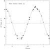 |
Fig. 1 Radial velocity curve of WDS 04352–0944 Aa. Filled circles and empty squares represent our data and the velocities measured by NA85, respectively. Continuous line shows the orbital fitting. Dashed line indicates the barycentre’s velocity. |
4.2. WDS 05247–5219
In this quadruple system, components A and B form a visual pair, whose most recent orbit has been calculated by Argyle et al. (2002). They found a period of 191 years and an eccentricity of 0.64, although they note that the validity of their orbit should be confirmed with new measurements. Based on the paper by NA85, star A is classified in the MSC as a double-lined spectroscopic binary, although its orbital parameters have not yet been determined. In the first hierarchical level, AB (HD 35 860) and component C (HD 35 859) form a common proper motion pair. According to the MSC, the coincidence of their radial velocities is additional evidence of their physical connection.
We obtained 20 spectra of the AB pair, in which surprisingly the spectral features of component B could not be detected. Taking the published brightness difference into account, we expected to detect the spectral lines of star B at least at phases of quadrature of the subsystem Aab, when the spectral lines of Aa and Ab are well separated from the centre-of-mass velocity. One possible explanation is that B is an object with high rotational velocity, whose spectral lines had been mistaken with modulations of the continuum. It could also be another subsystem, in which case the brightness of its individual components would be lower than measured for the visual B.
We measured preliminary values of radial velocities for both components of Aab by cross-correlations with an observed A1V-type template, which led to good correlation peaks for both components. In a first attempt, the spectral separation method was applied to fifteen well-resolved spectra. The remaining five spectra were included in subsequent iterations, once their radial velocities were determined well. In the final iterations, velocities were measured with errors smaller than 1 km s-1 in strongly blended spectra, in which one-dimensional cross correlations had produced only one broadened peak containing both components. In these calculations synthetic templates with Teff = 9750K and Teff = 8000K were used. As an illustration of the quality of the reconstructed spectra obtained for both components, Fig. 2 shows a small section of them and the selected templates.
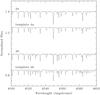 |
Fig. 2 Separated spectra of the components of WDS 05247–5219 Aab, compared with synthetic templates used to measure radial velocities. |
From the separated spectra we determined spectral types A1III and Am (calcium: A3; metals: A7) for the primary and secondary components of the SB2, respectively. Orbital parameters of this subsystem were calculated fitting by least squares the radial velocities for all the spectra (see Table 6). The orbital period was refined by adding the NA85’s data. Figure 3 shows the fitting of the radial velocities and compares NA85’s data with ours.
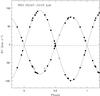 |
Fig. 3 Radial velocity curves of WDS 05247–5219 Aab. Filled circles and empty squares represent our data and the velocities measured by NA85, respectively. Continuous line shows the orbital fitting. Dashed line indicates the barycentre’s velocity. |
We obtained six spectra of HD 35 859 (=component C) with a time baseline of 1.55 years. We measured radial velocities by cross correlations using a template with Teff = 8750K and vsini = 200 km s-1. The measured velocities took values between +0.6 km s-1 and −10.2 km s-1, with errors of about 10 km s-1. The three measurements published by NA85 also lie in a similar velocity range, but since their formal error is about 3 km s-1, they classified it as suspected of variability. In any case, a variation in such amplitude in a high rotation star would be difficult to confirm. The mean velocity of this component is similar to the value obtained for the barycentre of Aab, as mentioned in the MSC. Furthermore, the proper motions given in the SPM4 catalogue (Girard et al. 2011) for the subsystem AB and star C agree within their errors.
4.3. WDS 08263–3904
Component A of this quadruple system is the eclipsing binary NO Puppis (HD 71 487) and component B is the primary of the visual double B1605 (HD 71 488). The variability of NO Puppis was discovered by Grønbech (Jorgensen 1972), who obtained the photometric elements from Strömgren ubvy light curves (Grønbech 1976). Gimenez et al. (1986) used these observational data along with new times of minima to determine the apsidal motion of the orbit, obtaining a rate of  deg/cyc (U = 37.2 yr). Furthermore, they confirmed the elements obtained by Grønbech for a radius-ratio Rb/Ra = 0.7. However, to date there have been no spectroscopic observations that allow absolute dimensions to be determined for the system.
We obtained 20 spectra of HD 71 487, and subsequently applied the method GL06 to separate the spectra of the components and measure their radial velocities. To calculate absolute parameters, we fitted our radial velocities and the photometric ubvy data published by Grønbech simultaneously, using the Wilson & Devinney code (Wilson & Devinney 1971; Wilson 1979, 1990). In this analysis, we fixed the apsidal motion rate at the value published by Gimenez et al. and fitted the remaining orbital (a,e,ω0,Vγ,i,T0,P) and physical (Tb,Ωa,Ωb,q) parameters of the components. In accordance with its spectral type, we adopted a temperature of 13 000 K for the primary component. To model the limb-darkening we used a linear law with coefficients selected from the tables by van Hamme (1993). As usual for stars with radiative envelopes, we adopted values of 1.0 for the exponent of the limb-darkening law and for the bolometric albedos of both components. Since the diaphragm used in the photoelectric observations of Grønbech includes light from HD 71 488, we fitted this additional flux contribution through the parameter l3 for each light curve.
As Grønbech pointed out, the photometric solution is very indeterminate. For this reason, simultaneous fitting of radial velocities and light curves did not lead to unambiguous potentials for both components. We therefore fixed the radius-ratio to Rb/Ra = 0.69, which is the value corresponding to the spectroscopic mass ratio according to main-sequence stellar models. This value depends slightly on the primary mass and age and was calculated in a second iteration after absolute parameters of the stars were calculated. Within this constraint we selected the solution corresponding to the best fit of the observational data, i.e., to the least rms deviation.
Figures 4 and 5 show the curve fitting for the light and radial velocities, respectively. The orbital parameters of this subsystem are given in Table 6. Additionally, we obtained an inclination i = 80.4 ± 0.2°. The eccentricity found agrees with the value obtained by Gimenez et al. from their apsidal motion analysis (e = 0.1255 ± 0.0010). Table 7 lists the physical parameters obtained for both components.
Grønbech proposed five alternative solutions for values Rb/Ra between 0.6 and 1.0 at regular intervals of 0.1. For each adopted ratio he fitted the four light curves separately. The simultaneous fitting in this work led to slightly lower values for the rms deviation of the data in all filters. In particular, the deviations calculated for the four light curves are between 5% and 10% less than those obtained by Grønbech for a ratio of radii of 0.7.
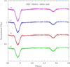 |
Fig. 4 Light curves of WDS 08263–3904 Aab. Open circles represent the measurements by Grønbech (1976) in filters ubvy. Continuous lines show the curve fittings to those data. |
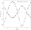 |
Fig. 5 Radial velocity curves of WDS 08263–3904 Aab. Filled circles represent our measurements. Continuous line shows the orbital fitting. Dashed line indicates the barycentre’s velocity. |
Radial velocities of double-lined spectroscopic binaries.
Orbital parameters of spectroscopic binary subsystems.
With the aim of determining the age and evolutionary state of HD 71 487, we compared the parameters obtained with theoretical models by Lejeune & Schaerer (2001) for solar composition. Figure 6 presents the mass-radius diagram for the components. The stellar components of this subsystem are very close to the zero-age main-sequence, and considering the parameters uncertainties, it can be asserted that it is younger than 107 years old.
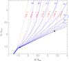 |
Fig. 6 Mass-radius diagram of the subsystem WDS 08263–3904 Aab. Filled circles with error bars represent the components, whose positions are compared with the models of Lejeune & Schaerer (2001) for solar composition. Isochrones corresponding to log τ = 6.5 and log τ = 7.0 are plotted in continuous and dashed lines, respectively. |
The eccentric character of the orbit is a very striking fact for such a short period binary. According to standard models for tidal circularization (Hut 1981), it is expected that the eccentricity is reduced to only 3% of its original value in 1 Myr. Despite its young age, the scenario in which the system formed as an eccentric binary and is at present evolving towards a circular configuration is very unlikely. In fact, going back in time, theoretical models predict that only 2.3 × 10⁵ yr ago the system would have had an eccentricity e = 0.55, high enough for the stars to collide at periastron. In conclusion, the present orbital configuration with a semiaxis of only 8.3 R⊙ seems to have been reached recently by some fast dynamical process. This dynamical event would involve the interaction with a third body. The large separation between NO Pup and stars B and C, the remaining components of this multiple, rule out the possibility that they have played such a role.
Physical parameters of the components of WDS 08263–3904 Aab.
Additional information about the dynamical history of the system can be derived from the stellar rotational velocities, since the timescale for the stellar rotation to synchronize with the orbital motion is even shorter than the circularization timescale. We measured rotational velocities in the separated spectra of star Aa and Ab by applying the method of the Fourier transform of the cross-correlation maximum developed by Díaz et al. (2011), obtaining vsinia = 86.5 ± 1.3 km s-1 and vsinib = 58.7 ± 0.6 km s-1. Using the orbital inclination and the stellar radii listed in Table 7, we obtained the rotational periods: Prot,a = 1.235 ± 0.019 d and Prot,b = 1.250 ± 0.015 d. According to tidal evolution models, before the orbit has been circularized, stellar rotation synchronizes with the pseudo-synchronization period (Hut 1981), which for this system equals Pps = 1.1492 ± 0.0006 d. Therefore, rotation and orbital motion are not pseudo-synchronized in this binary.
In contrast, we note that the rotation periods are instead indistinguishable from the orbital period, which equals the pseudo-synchronization period only for circular orbits. This would suggest a scenario in which the orbit had reached synchronization and circularization, and subsequently suffered a dynamical process that injects eccentricity into the system without modifying the orbital semiaxis. This is what happens in Kozai cycles, where the interaction of a close binary with a distant third body induces periodic oscillations in the binary eccentricity and inclination, keeping the semiaxis constant (Innanen et al. 1997; Ford et al. 2000). According to Makarov & Eggleton (2009), the effects are only significant if Pout(yr) ≲ [Pin(d)] 1.4. In the case of NO Pup, the hypothetical perturbing body would be orbiting the binary with Pout < 500 d, aout < 2.2 AU. The period of the eccentricity oscillations depends on the outer-to-inner period-ratio and on the relative mass of the third body. We speculate that if the third body is a low-mass star, the period of Kozai cycle could be long enough to allow the binary to synchronize with the orbital period during the low-eccentricity stage before the subsequent incursion on high eccentricities.
We obtained three spectra of HD 71 488 (=component B). We did not detect any morphological or radial velocity variations between them. These spectra were very much like a template with Teff = 9000K convolved with a rotational profile corresponding to vsini = 60 km s-1. We did not detect the spectral lines of the fainter component of this visual subsystem separately. This is consistent with the similarity between the spectral types given for components B and C in the MSC. The mean radial velocity of star B is 21.9 ± 1.6 km s-1, which supports the physical link between this visual subsystem and HD 71 487.
4.4. WDS 08563–5243
According to the MSC, this is a triple system whose components A and B form a visual pair, with A approximately 20 times brighter than B. Component A has been classified as a single-lined spectroscopic binary, so the third component of the system is its undetected companion. The orbital elements of this SB1 were published by Neubauer (1930) and subsequently corrected by Blanco & Tollinchi (1957). The published period is 0.9147 days and the eccentricity 0.13, which is an unusual value since with such a short period, the orbit would be expected to have been circularized by tidal effects.
Owing to the small separation and the large brightness difference between the components of the visual pair, we could not observe B. We obtained 24 spectra of A, which are slightly contaminated by the light of its faint visual companion. The lines of Ab, not detected in previous works, were clearly visible in 13 of our spectra. In the remaining, this component was blended with Aa. For detecting and measuring the radial velocity of the faintest component by cross-correlations, we used a template of spectral type A0V. The brighter component Aa could be measured reliably in 19 spectra using a B4V-type template. These measurements were used to fit the binary period and were combined with the velocities of Ab to obtain a preliminary orbit for the system.
This preliminary fitting was used to calculate radial velocities for all 24 spectra, which were adopted as starting values in the spectral separation process. In the latter we included all the spectra and measured final radial velocities for them. We used synthetic templates with Teff = 16 000 K, vsini = 50 km s-1, and Teff = 9500 K to measure the radial velocities of Aa and Ab, respectively.
From the radial velocity curves fitting, we obtained a circular orbit (e = 0.009 ± 0.010) with a period of 1.09766 days (Table 6). Figure 7 shows the radial velocity curves of Aa and Ab. As can be seen, good velocities for both components could be measured very close to conjunction phase thanks to applying the method of GL06.
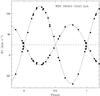 |
Fig. 7 Radial velocity curves of WDS 08563–5243 Aab. Filled circles represent our measurements. Continuous line shows the orbital fitting. Dashed line indicates the barycentre’s velocity. |
4.5. WDS 16054–1948
This system, also named β Scorpii, is formed by six components. In the first hierarchical level, the visual pairs AB (HD 144 217) and CE (HD 144 218) form a common proper motion system with a separation of 13.6′′. Seymour et al. (2002) calculated orbital elements for the AB pair and found a period of 610 years. The components of this pair have been widely studied, and for over 50 years it has been known that A is a double-lined spectroscopic binary (Abhyankar 1959). This binary has been studied in detail by Holmgren et al. (1997), who found a period of 6.8282 days and determined the remaining orbital parameters.
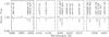 |
Fig. 8 Selected regions of the disentangled spectrum of HD 144 218 E showing lines of Mn, Ga, Zr, and Sr. |
Until the beginning of this investigation, detailed spectroscopic studies of the CE pair had not yet been published. The separation between C and E is 0.133′′ and, according to Evans et al. (1977), E is 2.1 mag fainter than its visual companion. Van Flandern & Espenschied (1975) measured unusual colours for E, from which they suggested that this component could be a double system or a peculiar star. More recently, the subsystem CE was analysed by Catanzaro (2010), who reported component E as a single-lined spectroscopic binary and found its orbital parameters. Furthermore, he carried out an abundance analysis using a high-resolution spectrum (R ≈ 70 000) of the visual subsystem. He measured overabundances of Hg and Sr, from which he suggested that Ea could be a HgMn star. Nevertheless, he admitted that the Hg ii line at λ3984 Å is confused with two blended lines belonging to component C. Mason et al. (2010) published the most recent orbit for the CE pair, with a period of 39 years. They classified that orbit as “reliable” based on the quantitative method by Hartkopf et al. (2001).
We obtained 14 spectra of the CE pair with a time baseline of almost five years. Like Catanzaro, we detected variability in the profiles of spectral lines of star C. Only a few spectral lines of star Ea could be detected in our spectra, among them Fe ii λ4549.549 Å, Ti ii λ4563.761 Å, and Ti ii λ4571.971 Å.
With the aim of disentangling the spectra of the components, we measured preliminary radial velocities by cross-correlations using a template with Teff = 20 000K and vsini = 60 km s-1 for star C. In the velocity measurements of star Ea, we include small spectral regions containing only the three lines mentioned above and employed a template with Teff = 13 000 K, the temperature found by Catanzaro for this component. The spectral morphology of the separated spectra was entirely consistent with the temperatures previously estimated for both components. It should be noted that the temperature found for C is somewhat lower than the value found by Catanzaro (24 000 ± 500 K).
From the separated spectra of C and Ea, we estimated spectral types B2V and B8pMn, respectively. In the spectra of Ea, we detected strong lines of Mn ii and other elements that are usually present in the atmospheres of HgMn stars, such as strontium, zirconium, and gallium. Nevertheless, we did not detect a conspicuous line Hg ii λ 3984 Å. We note that the presence of Zr ii and Ga ii lines, which are clearly visible in our spectra, had not been reported in the abundance analysis by Catanzaro. Figure 8 shows a few small spectral windows of the spectrum of HD 144 218 E, where lines of Cr ii (λ4145.8), Mn ii (λλ4000.0, 4205.4, 4206.4, 4248.0, 4251.7, 4253.0), Ga ii (λλ4251.1, 4255.7), Zr ii (λλ4149.2, 4209.0, 4210.6, 4211.9), and Sr ii (λλ4215.5) have been identified.
After removing the spectrum of Ea from the observed spectra, the morphological variations in the spectral lines of star C decreased significantly. Therefore, such variability is largely due to the overlapping of the moving spectral lines of Ea. However, time series of high-resolution spectroscopic observations would be useful for analysing that effect in detail.
By fitting the radial velocities of Ea, we obtained a preliminary orbit. Nevertheless, the centre-of-mass velocity of this binary is expected to vary, since it is part of a visual system. For a proper fitting of the orbit of the spectroscopic subsystem, it is necessary to correct the measured velocity by the velocity of the barycentre and also to correct the times of observation by the “light-time effect”. Both corrections are computed on the basis of the parameters of the visual orbit and the mass ratio between the components of the visual pair. In particular, the velocities measured for C, corrected by the motion in the visual orbit, should correspond to the velocity of the barycentre of CE.
While the visual orbit computed by Mason et al. for the CE pair is available, the mass ratio between Eab and C is unknown. We estimated masses for components C and Ea from their spectral types. Considering the published magnitude difference between C and E and the flux ratio between C and Ea obtained from ratios between their spectral lines, we estimated a temperature slightly lower for Eb than that of its spectroscopic companion. This led to a maximum mass ratio for Eab. On the other hand, we used the orbital parameters found for Ea to compute a minimum mass ratio for the spectroscopic subsystem. These two values defined a range of possible values for the mass ratio of the visual pair CE. We obtained a dynamical parallax of 5.0 mas, somewhat greater than the corresponding value given by Mason et al. (4.4 mas), but discordant with the Hipparcos parallax (8.2 ± 1.2 mas, van Leeuwen 2007). We used the parameters of the visual orbit to calculate the corrections to the radial velocities measured for Ea and C. For that, we assumed the dynamical parallax obtained and a mean value of 0.75 for the mass ratio of the CE pair.
Figure 9 shows the fitting of the radial velocities of Ea corrected by the motion of the barycentre. The rms deviation is 1.2 km s-1. The orbital parameters obtained for the subsystem Ea, given in Table 6, do not agree with those given by Catanzaro (P = 10.6851 ± 0.0006days,e = 0.25 ± 0.04, Vγ = −3.2 ± 1.3 km s-1,Ka = 37.5 ± 2.1 km s-1). For comparison, in Fig. 9 we overplot his 14 radial velocities, also corrected for the motion of the barycentre. From these measurements, 12 are distributed along a time baseline of about one year included in the time interval of our data. The other two values were measured by that author in two high-resolution spectra taken two and three years before. They correspond to the two points that clearly deviate from the fitting (phases 0.49 and 0.99). The rms deviation of the remaining 12 velocities of Catanzaro is 6.4 km s-1.
The velocities of C corrected by the motion in its visual orbit led to a mean value of −7.9 ± 1.0 km s-1, which differs significantly from the velocity of the barycentre of CE obtained from the fit of the spectroscopic orbit. This disagreement, together with the discrepancy in the parallax, suggest that the visual orbit should possibly be revisited.
4.6. WDS 17301–3343
Components A and B of this system form a common radial velocity pair separated by 4.44′′. The system is catalogued as triple in the MSC since A has been classified as a single-lined spectroscopic binary. We could not observe star B because it is 3 mag fainter than its companion and is located at a distance comparable to the typical seeing at the 2.15 m telescope site at CASLEO.
Penny et al. (1975) calculated the orbit of the binary subsystem, with a period of 38.1 days, but their data are of low quality. To improve the orbit and eventually detect the secondary component, we obtained a relatively large number observations of this subsystem: 28 spectra in 9 observing runs over approximately 5 years. The spectral features of the secondary component, however, could not been detected.
We measured radial velocities using a template of spectral type B0 convolved with a rotational profile of vsini = 80 km s-1. The velocity formal error was typically 2 km s-1. Our data are not consistent with the period found by Penny et al. For each observing run, the velocities remained constant within the measurement error. Therefore, in spite of having a considerable number of spectra, the identification of the orbital period was difficult because in practice we only had eight data points corresponding to the mean velocity for each observing run. For this reason, we complemented our data with the velocities published by Thackeray et al. (1973) and Buscombe & Kennedy (1969). We obtained a preliminary orbit with a period of about 258 days. Figure 10 shows the fitting of the radial velocities. Table 6 lists the orbital parameters obtained. The rms deviation of our velocities is 1.3 km s-1. However, it should be mentioned that another possible orbit, with a period of about 842 days, is also consistent with the observational data. We plan to carry out new observations with the aim of testing the validity of the calculated orbit.
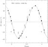 |
Fig. 9 Radial velocity curve of WDS 16054–1948 Ea. Filled circles represent the values measured in this investigation, which were used to obtain the orbital solution. Empty squares represent the radial velocities measured by Catanzaro (2010). Continuous line shows the orbital fitting. Dashed line indicates the barycentre’s velocity. |
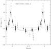 |
Fig. 10 Radial velocity curve of WDS 17301–3343 Aa. Filled circles represent our measurements. Empty squares represent the radial velocities measured by Thackeray et al. (1973) and Buscombe & Kennedy (1969). Continuous line shows the orbital fitting. Dashed line indicates the barycentre’s velocity. |
5. Discussion
The hierarchical configuration of the six analysed systems is presented in Fig. 11 in a similar manner to Tokovinin (2008). Some analysed systems are highly hierarchical, with ratios between outer and inner periods higher than 104. These configurations could be result of the contraction of the inner orbit as a consequence of some migration mechanism. However, in some cases there might be intermediate hierarchical levels that have not been detected to date. Detecting such intermediate orbits is difficult, since it requires either spectroscopic observations with a long time baseline or very high-resolution images. It is therefore interesting to evaluate our detection limits of intermediate orbits, which allows us to estimate the completeness in the knowledge of the multiplicity and structure of the analysed systems achieved through this study.
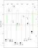 |
Fig. 11 Configuration of the analysed multiple systems: a) WDS 04352–0944, b) WDS 05247–5219, c) WDS 08263–3904, d) WDS 08563–5243, e) WDS 16054–1948, and f) WDS 17301–3343. Stellar components are represented by circles. Filled circles are stars observed in the present paper. No symbol is plotted for stellar components that are not visible in the spectrum (secondaries of SB1 systems). Dashed lines divide approximately the period axis in spectroscopic (S), visual (V), and common proper motion (C) ranges. The size of the circles roughly scale with the stellar mass. Green thick lines mark separation intervals that have not been investigated and might harbour additional hierarchical levels. |
For each multiple system studied, we calculated the probability that the presence of a body in an intermediate subsystem has gone unnoticed in our study, i.e. the probability that its perturbation on the inner subsystem was not detected in our velocity measurements. To this aim we first derived an expression for the radial velocity amplitude of the barycentre of the inner binary as a function of perturbing mass, outer period, and orbital inclination, adopting a circular outer orbit. Then, considering the temporal extent of our observations for each particular system and assuming random distributions for the orbital inclinations and for the orbital phase of the beginning of the observation window, we analytically derived the probability that the radial velocity variations of the inner binary center-of-mass are smaller than its observational error.
Figure 12 shows the detection probability of intermediate orbits in the parameter space. Each system is presented in a panel of this figure. Although the minimal value for the ratio Pout/Pin in a hierarchical system depends on the characteristics of each particular system (Mardling & Aarseth 2001), we adopted a conservative value of 10 in all cases to delimit the range of possible periods for the intermediate orbit to maintain the stability of the system. Therefore, if Pout and Pin are the periods of known outer and inner adjacent orbits, there may be an intermediate orbit with period P only if it fulfils the condition log Pin + 1 ≤ log P ≤ log Pout − 1. If the intermediate orbit is located to the right of the line corresponding to the upper limit for Pout for the existence of Kozai cycles, the third body would not influence the dynamical evolution of the inner subsystem. To indicate the completeness of this study, we represent detection probabilities of 95% and 50% respectively. The 0.15″ separation line corresponds to a typical lower limit that could be achieved through visual observations for stars with a magnitude difference Δm ≲ 4 using techniques such as speckle interferometry or adaptive optics (Mason et al. 2011; Tokovinin et al. 2010a).
The top panels of Fig. 12 show the detection limits for the systems WDS 05247–5219 (left) and WDS 16054–1948 (right). In both cases, this study has essentially covered the whole period range that could have a hypothetical intermediate orbit between the analysed inner subsystem and the corresponding visual pair, considering the stability condition of the system. In the case of WDS 05247–5219, for example, not detecting radial velocity variations of the barycentre of the subsystem Aab, in combination with the speckle observations carried out by Tokovinin et al. (2010b) that did not reveal new companions with separations down to the visual limit indicated in the graphics (ρ = 0.15″ for Δm = 4), indicates that additional hierarchical levels between the spectroscopic binary Aab and the visual pair AB is hardly likely to exist. Therefore, a fairly complete knowledge of this multiple system is currently available, as a result of the use of different observations techniques. However, it would be interesting to continue with the spectroscopic observations of component C to establish that this object is radial velocity variable, in which case the system would have an additional component.
Similarly, it is also unlikely that there is an intermediate hierarchical level between the spectroscopic subsystem Eab and the visual pair CE of WDS 16054–1948. We did not carry out an observational monitoring of the others visual components (A and B) of WDS 16054–1948 since they already had spectroscopic studies. Recently, Mason et al. (2010) measured the CE pair and corrected the calculated orbit. Nevertheless, the available observations of the AB pair covers only one third of the orbit obtained by Seymour et al. (2002). Therefore, new visual observations of this subsystem are required, both to refine its orbit and to verify the existence of intermediate hierarchies between this visual pair and the spectroscopic subsystem Aab.
The middle panels of Fig. 12 correspond to the systems WDS 04352–0944 (left) and WDS 08563–5243 (right). In the former case we adopted a maximum mass of 1 M⊙ for the secondary component of the subsystem HD 29 173. For both systems, this spectroscopic investigation has enabled us to rule out almost completely the existence of intermediate hierarchies with separations below the visual limit. In particular, we can assert that there are no additional companions that may be influencing the dynamical evolution of the inner subsystems. However, there are no high-resolution visual studies of these systems. In the case of WDS 08563–5243, the speckle observations carried out by Mason et al. (2011) did not reveal the existence of new companions with separations down to about 1″. Visual observations with resolution better than 1″, using techniques such as adaptive optics, speckle interferometry, or lucky imaging (Maíz Apellániz 2010), are needed to complete the search of intermediate orbits in these systems.
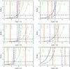 |
Fig. 12 Detection limits of intermediate orbits for the systems WDS 05247–5219 (top left), WDS 16054–1948 (top right), WDS 04352–0944 (middle left), WDS 08563–5243 (middle right), WDS 08263–3904 (bottom left), and WDS 17301–3343 (bottom right). Thick red vertical continuous lines delimit the range of possible periods for the intermediate orbit to maintain the stability of the system. The thick blue vertical dot-dashed line represents the upper limit for Pout for the existence of Kozai cycles (Pout(yr) ≲ [Pin(days)] 1.4). Thick black continuous and long-dashed curves indicate detection probabilities of 95% and 50%, respectively. The corresponding thin lines represent detection probabilities of 95% and 50% that would be achieved if we extend the time baseline of the observations indefinitely. Thin green dotted lines are references to the angular separations that would have the components for some periods, considering the parallax of the system. Thick black vertical and horizontal dashed lines indicate a separation of ρ = 0.15′′ and the mass of the third body corresponding to a magnitude difference Δm = 4 with the spectroscopic subsystem (see explanation in the text). |
Even if we extended indefinitely the time baseline of the observations, our study would not allow to obtain a secure knowledge of the multiplicity down to the visual limit of the systems WDS 08263–3904 and WDS 17301–3343. As can be seen in the left bottom panel of Fig. 12, the detection limits of intermediate orbits in WDS 08263–3904 are restricted to periods of some hundreds of days due to the briefness of the time baseline of the observations. However, we can state with a probability of about 50% that there are not companions able to affect the dynamical evolution of the spectroscopic subsystem. The speckle observations of Tokovinin et al. (2010b) and Hartkopf et al. (2012) did not reveal any additional hierarchies with separations down to the visual limit. On the other hand, the knowledge of the system WDS 17301–3343 is rather incomplete, as shown in the bottom right panel of Fig. 12. The low sensitivity to the presence of an additional companion in an intermediate orbit is directly related to the relative high mass of the spectroscopic subsystem Aab. According to its spectral type, the primary component Aa has a mass of about 17 M⊙, so the total mass of the subsystem would be approximately 20 M⊙, which increases the minimum mass that a perturber body should have in order to produce a detectable variation in the barycentric velocity of Aab. Furthermore, there are no high-resolution observations of this system either. Therefore, an intermediate hierarchy level orbit might exist between AB and Aab with a period between a few thousand and a few million years, as well as undetected companions of B.
6. Conclusions
In this paper we have presented the results of a spectroscopic study of six multiple systems containing previously catalogued spectroscopic subsystems. For three of them (WDS 04352–0944 Aab, WDS 05247–5219 Aab, WDS 08263–3904 Aab), we determined orbital elements for the first time. For the other three we obtained, on the basis of our observations, orbital parameters with higher accuracy than previously published. In the systems WDS 04352–0944, WDS 05247–5219, and WDS 08563–5243, we kinematically confirmed the physical link between the spectroscopic subsystem and its visual companion.
The periods obtained for the inner subsystems confirm that these systems are hierarchical, considering the parameters published in the MSC for the wider orbits. In particular, WDS 04352–0944, WDS 08263–3904, and WDS 08563–5243 show ratios Pout/Pin greater than 105 with inner periods shorter than six days. In these cases, the inner subsystems could have experienced some migration mechanism that led them to their present orbits (Tokovinin 2008). We speculate that in the case of WDS 08263–3904, a dynamical interaction with a low-mass undetected companion might also be responsible for the eccentric character of the inner orbit. However, for WDS 04352–0944 and WDS 08563–5243, there is no companion with appreciable mass (≳0.5 M⊙) that could have played such a role via Kozai cycles. This can also be argued for the system WDS 05247–5219, considering companions with mass greater than approximately 1 M⊙. Particularly, for the latter and WDS 16054–1948 CE, we can exclude the existence of additional components with masses greater than 1.5 M⊙ in intermediate levels.
This study has shown that the analysis of spectroscopic observations over a long time baseline is particularly useful and, in many cases, irreplaceable for detecting those intermediate hierarchical levels that could play a role in the dynamical formation of close binary subsystems. These ranges of intermediate periods are often out of reach of visual observations, as is the case for five of the six systems analysed in this paper.
Acknowledgments
This paper was partially supported by a grant from FONCyT-UNSJ PICTO-2009-0125. We are grateful to Natalia Nuñez and Ana Collado, who kindly took some spectra used in this investigation.
References
- Abhyankar, K. D. 1959, ApJS, 4, 157 [NASA ADS] [CrossRef] [Google Scholar]
- Argyle, R. W., Alzner, A., & Horch, E. P. 2002, A&A, 384, 171 [NASA ADS] [CrossRef] [EDP Sciences] [Google Scholar]
- Bertone, E., Buzzoni, A., Chávez, M., & Rodríguez-Merino, L. H. 2008, A&A, 485, 823 [NASA ADS] [CrossRef] [EDP Sciences] [Google Scholar]
- Blanco, V., & Tollinchi, E. 1957, PASP, 69, 354 [NASA ADS] [CrossRef] [Google Scholar]
- Buscombe, W., & Kennedy, P. M. 1969, MNRAS, 143, 1 [NASA ADS] [CrossRef] [Google Scholar]
- Catanzaro, G. 2010, A&A, 509, A21 [NASA ADS] [CrossRef] [EDP Sciences] [Google Scholar]
- Chini, R., Hoffmeister, V. H., Nasseri, A., Stahl, O., & Zinnecker, H. 2012, MNRAS, 424, 1925 [NASA ADS] [CrossRef] [Google Scholar]
- Chini, R., Barr, A., Buda, L. S., et al. 2013, Central European Astrophysical Bulletin, 37, 295 [NASA ADS] [Google Scholar]
- Díaz, C. G., González, J. F., Levato, H., & Grosso, M. 2011, A&A, 531, A143 [NASA ADS] [CrossRef] [EDP Sciences] [Google Scholar]
- Duchêne, G., & Bouvier, J. 2008, in Multiple Stars Across the H-R Diagram, eds. S. Hubrig, M. Petr-Gotzens, & A. Tokovinin, 219 [Google Scholar]
- Duchêne, G., & Kraus, A. 2013, ARA&A, 51, 269 [Google Scholar]
- Evans, D. S., Africano, J. L., Fekel, F. C., et al. 1977, AJ, 82, 495 [NASA ADS] [CrossRef] [Google Scholar]
- Ford, E. B., Kozinsky, B., & Rasio, F. A. 2000, ApJ, 535, 385 [NASA ADS] [CrossRef] [Google Scholar]
- Gimenez, A., Clausen, J. V., & Jensen, K. S. 1986, A&A, 159, 157 [NASA ADS] [Google Scholar]
- Girard, T. M., van Altena, W. F., Zacharias, N., et al. 2011, AJ, 142, 15 [NASA ADS] [CrossRef] [Google Scholar]
- González, J. F., & Levato, H. 2006, A&A, 448, 283 [NASA ADS] [CrossRef] [EDP Sciences] [Google Scholar]
- Grønbech, B. 1976, A&A, 50, 79 [NASA ADS] [Google Scholar]
- Hartkopf, W. I., Mason, B. D., & Worley, C. E. 2001, AJ, 122, 3472 [NASA ADS] [CrossRef] [Google Scholar]
- Hartkopf, W. I., Tokovinin, A., & Mason, B. D. 2012, AJ, 143, 42 [NASA ADS] [CrossRef] [Google Scholar]
- Holmgren, D., Hadrava, P., Harmanec, P., Koubsky, P., & Kubat, J. 1997, A&A, 322, 565 [NASA ADS] [Google Scholar]
- Hut, P. 1981, A&A, 99, 126 [NASA ADS] [Google Scholar]
- Innanen, K. A., Zheng, J. Q., Mikkola, S., & Valtonen, M. J. 1997, AJ, 113, 1915 [NASA ADS] [CrossRef] [Google Scholar]
- Jorgensen, B. G. 1972, IBVS, 641, 1 [NASA ADS] [Google Scholar]
- Kouwenhoven, M. B. N., Brown, A. G. A., Portegies Zwart, S. F., & Kaper, L. 2007, A&A, 474, 77 [NASA ADS] [CrossRef] [EDP Sciences] [Google Scholar]
- Lejeune, T., & Schaerer, D. 2001, A&A, 366, 538 [NASA ADS] [CrossRef] [EDP Sciences] [Google Scholar]
- Maíz Apellániz, J. 2010, A&A, 518, A1 [NASA ADS] [CrossRef] [EDP Sciences] [Google Scholar]
- Makarov, V. V., & Eggleton, P. P. 2009, ApJ, 703, 1760 [NASA ADS] [CrossRef] [Google Scholar]
- Mardling, R. A., & Aarseth, S. J. 2001, MNRAS, 321, 398 [NASA ADS] [CrossRef] [Google Scholar]
- Mason, B. D., Wycoff, G. L., Hartkopf, W. I., Douglass, G. G., & Worley, C. E. 2001, AJ, 122, 3466 [Google Scholar]
- Mason, B. D., Hartkopf, W. I., Gies, D. R., Henry, T. J., & Helsel, J. W. 2009, AJ, 137, 3358 [NASA ADS] [CrossRef] [EDP Sciences] [Google Scholar]
- Mason, B. D., Hartkopf, W. I., & Tokovinin, A. 2010, AJ, 140, 735 [NASA ADS] [CrossRef] [Google Scholar]
- Mason, B. D., Hartkopf, W. I., & Wycoff, G. L. 2011, AJ, 142, 46 [NASA ADS] [CrossRef] [Google Scholar]
- Neubauer, F. J. 1930, PASP, 42, 354 [NASA ADS] [CrossRef] [Google Scholar]
- Nordstrom, B., & Andersen, J. 1985, A&AS, 61, 53 [NASA ADS] [Google Scholar]
- Penny, A. J., Penfold, J. E., & Balona, L. A. 1975, MNRAS, 171, 387 [NASA ADS] [Google Scholar]
- Sana, H., & Evans, C. J. 2011, in IAU Symp. 272, eds. C. Neiner, G. Wade, G. Meynet, & G. Peters, 474 [Google Scholar]
- Schöller, M., Correia, S., Hubrig, S., & Ageorges, N. 2010, A&A, 522, A85 [NASA ADS] [CrossRef] [EDP Sciences] [Google Scholar]
- Seymour, D. M., Mason, B. D., Hartkopf, W. I., & Wycoff, G. L. 2002, AJ, 123, 1023 [NASA ADS] [CrossRef] [Google Scholar]
- Thackeray, A. D., Tritton, S. B., & Walker, E. N. 1973, MmRAS, 77, 199 [NASA ADS] [Google Scholar]
- Tokovinin, A. 2004, Rev. Mex. Astron. Astrofis., 21, 7 [Google Scholar]
- Tokovinin, A. 2008, MNRAS, 389, 925 [NASA ADS] [CrossRef] [Google Scholar]
- Tokovinin, A., Thomas, S., Sterzik, M., & Udry, S. 2006, A&A, 450, 681 [NASA ADS] [CrossRef] [EDP Sciences] [Google Scholar]
- Tokovinin, A., Hartung, M., & Hayward, T. L. 2010a, AJ, 140, 510 [NASA ADS] [CrossRef] [Google Scholar]
- Tokovinin, A., Mason, B. D., & Hartkopf, W. I. 2010b, AJ, 139, 743 [NASA ADS] [CrossRef] [Google Scholar]
- Tokovinin, A. A. 1997, A&AS, 124, 75 [NASA ADS] [CrossRef] [EDP Sciences] [Google Scholar]
- Tokovinin, A. A., & Smekhov, M. G. 2002, A&A, 382, 118 [NASA ADS] [CrossRef] [EDP Sciences] [Google Scholar]
- Van Flandern, T. C., & Espenschied, P. 1975, ApJ, 200, 61 [NASA ADS] [CrossRef] [Google Scholar]
- van Hamme, W. 1993, AJ, 106, 2096 [NASA ADS] [CrossRef] [Google Scholar]
- van Leeuwen, F. 2007, A&A, 474, 653 [NASA ADS] [CrossRef] [EDP Sciences] [Google Scholar]
- Wilson, R. E. 1979, ApJ, 234, 1054 [NASA ADS] [CrossRef] [Google Scholar]
- Wilson, R. E. 1990, ApJ, 356, 613 [NASA ADS] [CrossRef] [Google Scholar]
- Wilson, R. E., & Devinney, E. J. 1971, ApJ, 166, 605 [NASA ADS] [CrossRef] [Google Scholar]
All Tables
All Figures
|
Fig. 1 Radial velocity curve of WDS 04352–0944 Aa. Filled circles and empty squares represent our data and the velocities measured by NA85, respectively. Continuous line shows the orbital fitting. Dashed line indicates the barycentre’s velocity. |
| In the text | |
|
Fig. 2 Separated spectra of the components of WDS 05247–5219 Aab, compared with synthetic templates used to measure radial velocities. |
| In the text | |
|
Fig. 3 Radial velocity curves of WDS 05247–5219 Aab. Filled circles and empty squares represent our data and the velocities measured by NA85, respectively. Continuous line shows the orbital fitting. Dashed line indicates the barycentre’s velocity. |
| In the text | |
|
Fig. 4 Light curves of WDS 08263–3904 Aab. Open circles represent the measurements by Grønbech (1976) in filters ubvy. Continuous lines show the curve fittings to those data. |
| In the text | |
|
Fig. 5 Radial velocity curves of WDS 08263–3904 Aab. Filled circles represent our measurements. Continuous line shows the orbital fitting. Dashed line indicates the barycentre’s velocity. |
| In the text | |
|
Fig. 6 Mass-radius diagram of the subsystem WDS 08263–3904 Aab. Filled circles with error bars represent the components, whose positions are compared with the models of Lejeune & Schaerer (2001) for solar composition. Isochrones corresponding to log τ = 6.5 and log τ = 7.0 are plotted in continuous and dashed lines, respectively. |
| In the text | |
|
Fig. 7 Radial velocity curves of WDS 08563–5243 Aab. Filled circles represent our measurements. Continuous line shows the orbital fitting. Dashed line indicates the barycentre’s velocity. |
| In the text | |
|
Fig. 8 Selected regions of the disentangled spectrum of HD 144 218 E showing lines of Mn, Ga, Zr, and Sr. |
| In the text | |
|
Fig. 9 Radial velocity curve of WDS 16054–1948 Ea. Filled circles represent the values measured in this investigation, which were used to obtain the orbital solution. Empty squares represent the radial velocities measured by Catanzaro (2010). Continuous line shows the orbital fitting. Dashed line indicates the barycentre’s velocity. |
| In the text | |
|
Fig. 10 Radial velocity curve of WDS 17301–3343 Aa. Filled circles represent our measurements. Empty squares represent the radial velocities measured by Thackeray et al. (1973) and Buscombe & Kennedy (1969). Continuous line shows the orbital fitting. Dashed line indicates the barycentre’s velocity. |
| In the text | |
|
Fig. 11 Configuration of the analysed multiple systems: a) WDS 04352–0944, b) WDS 05247–5219, c) WDS 08263–3904, d) WDS 08563–5243, e) WDS 16054–1948, and f) WDS 17301–3343. Stellar components are represented by circles. Filled circles are stars observed in the present paper. No symbol is plotted for stellar components that are not visible in the spectrum (secondaries of SB1 systems). Dashed lines divide approximately the period axis in spectroscopic (S), visual (V), and common proper motion (C) ranges. The size of the circles roughly scale with the stellar mass. Green thick lines mark separation intervals that have not been investigated and might harbour additional hierarchical levels. |
| In the text | |
|
Fig. 12 Detection limits of intermediate orbits for the systems WDS 05247–5219 (top left), WDS 16054–1948 (top right), WDS 04352–0944 (middle left), WDS 08563–5243 (middle right), WDS 08263–3904 (bottom left), and WDS 17301–3343 (bottom right). Thick red vertical continuous lines delimit the range of possible periods for the intermediate orbit to maintain the stability of the system. The thick blue vertical dot-dashed line represents the upper limit for Pout for the existence of Kozai cycles (Pout(yr) ≲ [Pin(days)] 1.4). Thick black continuous and long-dashed curves indicate detection probabilities of 95% and 50%, respectively. The corresponding thin lines represent detection probabilities of 95% and 50% that would be achieved if we extend the time baseline of the observations indefinitely. Thin green dotted lines are references to the angular separations that would have the components for some periods, considering the parallax of the system. Thick black vertical and horizontal dashed lines indicate a separation of ρ = 0.15′′ and the mass of the third body corresponding to a magnitude difference Δm = 4 with the spectroscopic subsystem (see explanation in the text). |
| In the text | |
Current usage metrics show cumulative count of Article Views (full-text article views including HTML views, PDF and ePub downloads, according to the available data) and Abstracts Views on Vision4Press platform.
Data correspond to usage on the plateform after 2015. The current usage metrics is available 48-96 hours after online publication and is updated daily on week days.
Initial download of the metrics may take a while.