© ESO, 2014

1. Introduction

The present-day large-scale structure in cosmological matter distribution is formed by the gravitational amplification of small density perturbations that are a relic of the early Universe. The amplitude of these fluctuations as a function of scale carries unique information about the fundamental cosmological parameters, which describe the dominant constituents of the Universe and their densities with the global expansion history. Since the primordial density field is commonly thought to be a random Gaussian process, the Fourier power spectrum, or, its real-space counterpart, the correlation function provide a complete statistical description. Linear growth of small fluctuations preserves the shape of both, suggesting that observations of the large-scale structure today should still be able to extract pristine cosmological information.

This idealized picture is complicated in practice, as galaxies do not faithfully trace the distribution of matter but are undoubtedly biased to some extent. The reason this is inevitable is because galaxies form within dark matter haloes, and the more massive haloes form at special places within the cosmic density field. This generates a large-scale linear bias that gives a two-point correlation function, ξ(r), of galaxies that is related to that of mass by: (1)where the bias parameter, b, depends on halo mass (Kaiser 1984; Mo & White 1996; Sheth & Tormen 1999).

On small scales where the correlations are non-linear, the correlation function gains additional contributions, which arise from pairs within haloes that are massive enough to host more than one galaxy. Thus, the galaxy correlation function varies in shape and amplitude for different classes of galaxies because different classes of galaxy occupy different masses of haloes to different extents, and the distribution of galaxies within each halo does not necessary follow that of the mass (this is the basis of the “halo model” – see e.g. Cooray & Sheth 2002). Weak non-linearities in the mapping between the underlying matter density field and the distribution of collapsed objects also develop on quasi-linear scales (Sigad & Tormen 2000; Marinoni et al. 2005), as a consequence of the complex interplay between galaxy formation processes and gravitational dynamics. Additionally, there may be some scatter in the galaxy properties found in a set of haloes of the same mass; these effects are collected under the heading of “stochastic bias” (e.g. Dekel & Lahav 1999; Gao & White 2007) and have been shown to be small but non-zero in the observed galaxy distribution (e.g. Wild et al. 2005).

The non-linear physics responsible for galaxy formation can be mitigated by surveys covering large volumes, which can probe the power spectrum closer to the linear regime, or by focussing on robust features such as baryonic acoustic oscillations (BAO), the relic of the baryon-photon interactions in the pre-recombination plasma. These strategies have motivated the large “low-redshift” surveys of the past decade (e.g SDSS-3 BOSS, Eisenstein et al. 2011; Anderson et al. 2012; WiggleZ, Drinkwater 2010; Blake et al. 2011; 2dFGRS, Colless et al. 2001) and are also a major driver for the next generation of projects from the ground or space (e.g. BigBoss Schlegel et al. 2011; Euclid Laureijs 2011).

The development of multi-object spectrographs on 8-m class telescopes during the 1990s triggered a number of deep redshift surveys with measured distances beyond z ~ 0.5 over areas of 1–2 deg² (e.g. VVDS, Le Fèvre et al. 2005; DEEP2, Newman et al. 2013 and zCOSMOS, Lilly et al. 2009). Even so, it was not until the wide extension of VVDS was produced (Garilli et al. 2008) that a survey existed with sufficient volume to attempt cosmologically meaningful computations at z ~ 1 (Guzzo et al. 2008). In general, clustering measurements at z ≃ 1 from these samples remained dominated by cosmic variance, as dramatically shown by the discrepancy observed between the VVDS and zCOSMOS correlation functions at z ≃ 0.8 (de la Torre et al. 2010).

The VIMOS Public Extragalactic Redshift Survey (VIPERS) is part of this global attempt to take cosmological measurements at z ~ 1 to a new level in terms of statistical significance. In contrast to the BOSS and WiggleZ surveys, which use large-field-of-view (~1 deg²) fibre optic positioners to probe huge volumes at low sampling density, VIPERS exploits the features of VIMOS at the ESO VLT to yield a dense galaxy sampling over a moderately large field of view (~0.08 deg²). It reaches a volume at 0.5 < z < 1.2, which is comparable to that of the 2dFGRS (Colless et al. 2001) at z ~ 0.1, allowing the cosmological evolution to be tested with small statistical errors.

In parallel to improving the samples, we can try and devise statistical estimators that are capable of probing the density field, while being weakly sensitive to galaxy bias and non-linear evolution (e.g. Zhang et al. 2007; Bel & Marinoni 2012). This is the motivation for a new statistic introduced by Bel & Marinoni (2014; hereafter BM13), who proposed the use of the clustering ratio η_g,R(r), the ratio of the correlation function to the variance of the galaxy over-density field δ_R smoothed on a scale R. BM13 argue that this statistic has a redshift-space form that is independent of the specific bias of the galaxies used and is essentially only sensitive to the shape of the non-linear real-space matter power spectrum in two relatively narrow bandwidths.

BM13 have used numerical simulations to thoroughly discuss the level of precision reachable through this method on large linear scales. In particular, they showed that the clustering ratio measured from the simulations differs from the theoretical prediction by only 0.1% for some specific choices of the scales R and r that are involved in the smoothing of the auto-correlation of the galaxy density field. They also applied this technique to the SDSS-DR7 Luminous Red Galaxy sample with z < 0.4 by obtaining an estimate of the present matter density (Ω_m,0 = 0.283 ± 0.023), which is 20% more precise than the measurement of Percival et al. (2010) from a BAO analysis of the same sample. This demonstrates the sensitivity of relative clustering measurements made on different scales to Ω_m,0, which controls the horizon scale at matter-radiation equality and the corresponding turn-over in the growth rate of fluctuations.

The η statistics remains sensitive to non-linearities if we probe small enough scales. Since the statistical errors decline as we add small-scale data, there is a careful balance to be struck in attaining a result that has a small error bar, while lacking significant systematic errors. Non-linearities in themselves are unimportant, since the non-linear evolution of the matter power spectrum is in effect a solved problem at the level of precision we need and can be predicted for any model we wish to test. The non-trivial problem is eventually inadequate for the local bias hypothesis (Fry & Gaztañaga 1993) – i.e., a possible dependence of the bias parameter on the separation scale r (cf. Eq. (1)). We address this issue carefully in the present paper, using realistic simulated galaxy distributions, and show that the likely degree of scale dependence of the biasing relation in Fourier space is small enough that it does not constitute a significant uncertainty in the interpretation of our measurements of η.

In this paper, we measure the η_g,R statistic from the VIPERS Public Data Release 1 (PDR-1) redshift catalogue, by including ~64% of the final number of redshifts expected at completion (see Guzzo et al. 2013, hereafter Paper I, for a detailed description of the survey data set). The paper is organized as follows. In Sect. 2, we introduce the VIPERS survey and the features of the PDR-1 sample. In Sect. 3, we review the basics of the η-test, and we discuss how the galaxy clustering ratio is estimated from VIPERS data. In Sect. 4, we present the formalism that allows us to also predict the amplitude of this new cosmological observable in the non-linear regime, and we assess its overall viability with numerical simulations. This analysis helps us to identify the range of the parameter space where cosmological results can be meaningfully interpreted. In Sect. 5, we discuss the correction schemes adopted to account for the imprint of the specific VIPERS mask and selection effects, testing them with VIPERS mock surveys. Cosmological results are presented in Sect. 6 and conclusions are drawn in Sect. 7.

Throughout this paper, the Hubble constant is parameterized via h = H₀/100   km   s^-1   Mpc^-1, and all magnitudes in this paper are in the AB system (Oke & Gunn 1983). We do not give an explicit AB suffix. We do not fix cosmological parameters to a fiducial set of value. For consistency, we reconstruct the galaxy clustering ratio and analyse data in any tested cosmology.

2. Data

As already mentioned in this paper, we use the new data of the VIPERS, which is being built using the VIMOS spectrograph at the ESO VLT. The survey target sample is selected from the Canada-France-Hawaii Telescope Legacy Survey Wide (CFHTLS-Wide) optical photometric catalogues (Mellier et al. 2009). The VIPERS covers ~24 deg² on the sky divided over two areas within the W1 and W4 CFHTLS fields. Galaxies are selected to a limit of i_AB < 22.5, which further applies a simple and robust gri colour pre-selection, as to effectively remove galaxies at z < 0.5. Coupled to an aggressive observing strategy (Scodeggio et al. 2009), this allows us to double the galaxy sampling rate in the redshift range of interest with respect to a pure magnitude-limited sample (~40%). At the same time, the area and depth of the survey result in a fairly large volume, ~5 × 10⁷h^-3 Mpc³, analogous to that of the 2dFGRS at z ~ 0.1. Such combination of sampling and depth is quite unique over current redshift surveys at z > 0.5. The VIPERS spectra are collected with the VIMOS multi-object spectrograph (Le Fèvre et al. 2003) at moderate resolution (R = 210), using the LR Red grism, providing a wavelength coverage of 5500–9500Å and a typical redshift error of 141(1 + z) km s^-1. The full VIPERS area of ~24 deg² is covered through a mosaic of 288 VIMOS pointings (192 in the W1 area and 96 in the W4 area). A discussion of the survey data reduction and management infrastructure is presented in Garilli et al. (2012). An early subset of the spectra used here is analysed and classified through a Principal Component Analysis (PCA) in Marchetti et al. (2013).

A quality flag is assigned to each measured redshift based on the quality of the corresponding spectrum. Here and in all parallel VIPERS science analyses, we use only galaxies with flags 2 to 9 inclusive, which correspond to a global redshift confidence level of 98%. The redshift confirmation rate and redshift accuracy have been estimated using repeated spectroscopic observations in the VIPERS fields. A more complete description of the survey construction from the definition of the target sample to the actual spectra and redshift measurements is given in the parallel survey description paper (Paper I).

The data set used in this and the other papers is the VIPERS PDR-1 catalogue, which was made publicly available in September 2013. This includes 55,359 objects which are spread over a global area of 8.6 × 1.0 deg² and 5.3 × 1.5 deg², respectively, in W1 and W4. It corresponds to the data frozen in the VIPERS database at the end of the 2011/2012 observing campaign with 64% of the final expected survey yield. For the specific analysis presented here, the sample has been further limited to its higher-redshift part, selecting only galaxies with 0.65 < z < 1.2. The reason for this selection is related to the necessity of covering a minimum physical size in the declination direction, which, given the angular aperture of the survey, cannot be obtained for smaller distances (more details are given at the end of Sect. 3.2). This reduces the usable sample to 13 688 and 12 923 galaxies in W1 and W4, respectively (always with quality flag ≥2, as defined earlier). The corresponding volumes of the two samples are 1.3 and 1.2 × 10⁷h^-3 Mpc³ with a spanned largest linear dimension at z = 1.2 of ~400 and 250   h^-1   Mpc, respectively.

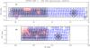Fig. 1 Distribution on the sky of the galaxies with measured redshifts in the VIPERS PDR-1 catalogue within the W1 and W4 fields (blue points). The pattern described by the gaps separating the VIMOS quadrants, as well as the areas not covered by the PDR-1, are clearly visible. Superimposed to the spectroscopic data, we also plot for illustrative purposes the projection of a subset of the spherical cells used to estimate the variance (regular grid on the left) with the typical motif used to estimate the 2-point correlation function of the smoothed density field ξg,R(r) (right). The spheres have a radius of R = 5   h-1   Mpc, and the chosen set is placed at redshift z = 0.66. Note that the distance between the centres of 2 opposite spheres in the motif is exactly equal to the chosen correlation scale r (we show here the case r = 3R). Red circles correspond to spheres that have been rejected in the clustering analysis because they are heavily affected by the survey mask (see discussion in Sect. 5.2.)

Open with DEXTER

3. Method

Here we briefly review the basic features of the clustering ratio cosmological test as proposed by BM13. We then discuss the procedure adopted to estimate it from a redshift survey like VIPERS.

3.1. The clustering ratio

Let δ_g,R(x) be the galaxy overdensity field that is smoothed on a scale R at the real-space position x (In the following, we assume that smoothing is done by convolving the field with a spherical Top Hat window of radius R). Its variance and 2-point correlation function ξ_g,R(r) =  ⟨ δ_g,R(x)δ_g,R(x + r) ⟩ _c (here ⟨ ... ⟩ _c indicates cumulant expectation values) can be combined to define the galaxy clustering ratio (p emphasis the dependency regarding to cosmological parameters). This statistic is a measure of the “slope” of the correlation function, which is smoothed over a particular double kernel structure (cf. Eq. (14) of Bel & Marinoni 2012). What is interesting about this statistic is that the galaxy clustering ratio and the mass clustering ratio in real space, which is defined as (2)coincide, or η_g,R(r,p) = η_R(r,p). This equality follows from the hypothesis that galaxy and mass density fields on a scale R are related via a linear local deterministic biasing scheme (Fry & Gaztañaga 1993). Note that, Ŵ is the Fourier transform of the smoothing window and is the dimensionless linear power spectrum of matter density fluctuations in Eq. (2). Two fundamental observations motivated the definition of the galaxy clustering ratio. Because it is a ratio between clustering at different scales, the clustering ratio is effectively insensitive to linear redshift distortions, which alter the amplitude of clustering in a way that is independent of phase or frequency (Kaiser 1987). We therefore have that (3)where quantities that are evaluated in redshift space are labelled with a tilde. Because the amplitude of the galaxy clustering is not affected by galaxy bias, we use this as the second salient feature of our definition.

The galaxy clustering ratio depends on the cosmological model through both the linear power spectrum in Eq. (2), which alters the right-hand-side (RHS) of Eq. (3) and the conversion applied to convert redshifts into distances, which alters the left-hand-side (LHS). The equivalence expressed by Eq. (3) holds true if and only if the LHS and RHS are both estimated in the “true” cosmological model. This is the basis of the “Alcock-Paczynski” approach to constraining the cosmological geometry (Alcock & Paczynski 1979; Ballinger et al. 1996; Marinoni & Buzzi 2010).

There are a few difficulties for the application of the clustering ratio test to the VIPERS data. The high density and small volume of the VIPERS survey mean that we can only accurately calculate the η statistic on smaller scales (typically R = 5   h^-1   Mpc) when compared to those for which this cosmological indicator was originally conceived. It is therefore necessary to extend the theoretical formalism of the η test to account for the effects of structure formation in the non-linear regimes. Adopting a non-linear power spectrum to predict the amplitude of the clustering ratio on these scales is necessary, but not sufficient. We must also properly incorporate a model for the non-linear redshift space distortion effect induced by the virial motions of galaxies into the theoretical framework, or the so-called Finger-of-God effect. The additional modelling required to extend the linear formalism of BM13 into the quasi-linear regime is presented and tested using simulations of the large scale structure in Sect. 4. Another concern is that results obtained on small scales might be more sensitive to a failure of a fundamental hypothesis on which the η formalism is built, or the locality of the biasing relation. Particular care is thus devoted to demonstrate via the analysis of numerical simulations that even the amplitude of the galaxy clustering ratio is not affected by using VIPERS galaxies as tracers on such small scales as R = 5   h^-1   Mpc. That is, it can be safely predicted without requiring the specification of a biasing scheme.

3.2. Estimating from VIPERS data

The estimation of the clustering ratio as a counts-in-cells statistic was presented in BM13. Here we review the measurement and describe the application to VIPERS data. , where N is the number of galaxies in spheres of radius R and its average value (we compute its value at the radial position r, corresponding to some look-back time t by averaging the cell counts within survey slices r ± 10R). These spheres tessellate the whole VIPERS survey in a regular way; their centres (called hereafter seeds) being located on a lattice of rectangular symmetry and spacing R (see Fig. 1). The 1-point, second order moment is measured as the variance (corrected for shot noise effects) of δ_N. The spheres partially include gaps in the survey due to the spacing of the VIMOS quadrants and to failed observations. Additionally, the sampling rate of the survey varies with the quadrant, as described in Paper I. The impact of these effects is investigated in Sect. 5.2.

To estimate the correlation function of the counts, we add a motif of isotropically distributed spheres around each seed (see right hand side of Fig. 1), and as proper seeds we retain only those for which the spheres of the motifs lie completely within the survey boundaries. The centre j of each new sphere is separated from the proper seed i by the length r = nR (where n is a generic real parameter usually taken without loss of generality to be an integer), and the pattern is designed in such a way as to maximize the number of quasi-non-overlapping spheres at the given distance r (the maximum allowed overlapping between contiguous spheres is 2% in volume). Incidentally, if the galaxy field is correlated on a scale r = 3R = 15   h^-1   Mpc, the number of spheres in a motif, or spheres isotropically placed around each proper seed is 26. ξ_g,R(r) is then estimated as ⟨ δ_Niδ_Nj ⟩, which is by averaging the counts over any cell i and j. In this last statistical quantity, note that we do not need to correct for shot noise since random sampling errors are uncorrelated. In Sect. 5.2, we discuss residual systematic effects arising from the survey geometry and sampling rate.

Considering cells of R = 5   h^-1   Mpc and after removing those cells that fall in bad or masked areas (see Sect. 5.2), the effective number of spheres used to estimate 1-point statistics is 68   667 in W1 and 58 684 in W4. Where 2-point statistics are concerned, the number of proper seeds is 37   814 in W1 and 39 459 in W4. Note that we can place more cells in W1 than in W4, since this last region is characterised by a smaller field of view. On the contrary, the number of proper seeds is larger in W4. This is explained by the angular shape of the field. The shallower extension in declination of W1 limits the number of motifs that we can fit inside the survey area. Since the error budget in the measurement of η_g,R is essentially dominated by the errors of the 2-point statistic, the clustering ratio is thus estimated in W4 with slightly higher precision. In this way, the small aperture of W1 also limits the effective redshift range we can probe. To be able to place an entire motif (see right hand side of top panel of Fig. 1) in W1, we need to restrict the analysis to redshifts above 0.65.

4. The clustering ratio in the non-linear regime

Because of the survey geometry, the galaxy clustering ratio can be precisely estimated from the VIPERS data only on relatively small scales, R < 8   h^-1   Mpc. It is thus necessary to generalize Eq. (3) to non-linear regimes and to test the validity of the hypothesis underlying such modelling. This entails additional assumptions with respect to the simple requirement of a deterministic biasing relation on a given smoothing scale R. Two distinct distortions must be modelled: linear theory over predicts the real space amplitude of the galaxy clustering ratio η_g,R in regimes of strong gravity, and the redshift-space amplitude of the galaxy clustering ratio is biased high with respect to η_g,R because of the Finger-of-God (FoG) effect (Jackson 1972; Tully & Fisher 1978). Concerns about these points can be addressed by using numerical simulations. We create these from the MultiDark simulation (Prada et al. 2012), a large flat ΛCDM simulation containing 2048³ particles, with mass of 8.721 × 10⁸   h^-1M_⊙ within a cube of side 1   h^-1   Gpc. The simulation starts at an initial redshift z_i = 65 with the following parameters: (Ω_m = 0.27,Ω_Λ = 0.73,H₀ = 70   km   s^-1   Mpc^-1,Ω_b = 0.0469,n_s = 0.95,σ₈ = 0.82). We match VIPERS against the time snapshot corresponding to z = 1 (although the sense of our conclusions is unchanged when other time outputs are considered in the analysis). This box (hereafter labelled B_h) contains nearly 14 millions haloes with mass M > 10^11.5   h^-1   M_⊙ and is used to check real-space properties of the clustering ratio with high statistical resolution.

We also consider a suite of 31 nearly independent light-cones, each extends over the redshift range 0.65 < z < 1.2 and covers a cosmological volume similar to that surveyed by the VIPERS PDR-1 data in the W4 field. These light-cones (hereafter indicated as L_h) incorporate redshift distortion effects, contain a total of ~10⁵ haloes each, and have a constant comoving radial density of objects, which is ~5 times higher than the mean effective density of galaxies in the VIPERS sample. These samples allow us to analyse the redshift space properties of the observable with great statistical resolution.

Note that the simulated haloes do not cover the whole range of masses in which the VIPERS galaxies are expected to reside, resulting in a different bias with respect to the real data. This is not expected to affect the realism of the tests performed, given that the η statistic is insensitive to linear galaxy bias. This aspect is discussed in depth in Sect. 4.3.

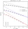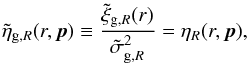
Fig. 2 Impact of non-linear clustering on the measurement and theoretical modelling of the galaxy clustering ratio η. The latter is measured in real space for the halo catalogues of the Bh simulation and compared to both the linear and non-linear predictions, as described respectively by a simple Eisenstein & Hu (1998) linear power spectrum (dot-dashed lines) and after correction through the non-linear HALOFIT prescription of Smith et al. (2003) (solid lines). The clustering ratio is shown as a function of the smoothing scale R adopted to filter the discrete distribution of haloes and for various correlation lengths (r = nR) with n =  { 2,3,4 }. Errors bars are obtained using 64 block-jackknife resampling of the data which excludes a cubic volume of linear size 250   h-1   Mpc each time.

Open with DEXTER

4.1. Non-linear effects in real space

We first explore whether the assumption of a simple phenomenological prescription for the amplitude and scaling of the matter power spectrum provided by Smith et al. (2003) is accurate enough for an effective implementation of the η-test with VIPERS data. We estimate the galaxy clustering ratio in real space (η_g,R(3R)) using the numerical simulations and compare them against the model given by the RHS of Eq. (2), which is calculated using either the linear power spectrum, or the non-linear model of Smith et al. (2003). Figure 2 shows the failure of the predictions based on a simple linear power spectrum model for the B_h halo box at z = 1. The amplitude of the clustering ratio is systematically over predicted on all R-scales and for all correlation lengths investigated. In contrast, the simple non-linear model of Smith et al. (2003) describes the data with greater accuracy over a wider interval of scales. On a scale as small as R = 5   h^-1   Mpc, the typical scale adopted to extract the maximum signal from VIPERS data, or the precision with which the amplitude of η_g,R(3R) is predicted is of order 3.6%,2.5% and 2.8% for the correlation scales n = 2,3, and 4, respectively. On scales R = 8   h^-1   Mpc and for the same correlation lengths, the relative discrepancy between theory and data is of order 1%,1.5%, and 2.5%, respectively.

These figures suggest that the remaining systematic error on the real-space model calculated by adopting the Smith et al. (2003) model is essentially negligible compared to the statistical uncertainty associated with current measurements of the clustering ratio η_g,R from VIPERS data (which is, δη/η ~ 10% at best when the field is filtered on the scale R = 5   h^-1   Mpc). Considering that the clustering ratio recovered on the correlation scale n = 2 and n = 4 is affected respectively by too large theoretical systematics (non-linearities in the power spectrum), by too large observational uncertainties (due to the shape of VIPERS fields), and in agreement with the analysis of BM13, we focus the rest of our analysis to the specific case, where the smoothed field is correlated on a scale r = 3R. Furthermore, we only consider the non-linear matter power spectrum model of Smith et al. (2003) from now on.

We remark that this analysis confirms the accuracy of the approximate relation (3) (upon implementation of a non-linear power spectrum model) even in regimes where σ_g,R is large. This is essentially due to the fact that, even on the small R-scales probed by VIPERS the second order coefficient of the bias relation is small with respect to the linear term.

4.2. Non-linear effects in redshift space

An interesting feature of Eq. (2) is that it is effectively insensitive to redshift distortions, and, therefore, independent of their specific modelling in the linear limit. This simplicity is lost when we consider small scales, R ~ 5   h^-1   Mpc, which are the typical scales probed by VIPERS, where non-linear motions are expected to contaminate the cosmological signal.

The existence of such effects is shown in Fig. 3, where we compare measurements of the galaxy clustering ratio for haloes selected in real space and in redshift space from the L_h simulations (η_g,R and , respectively). The discrepancy between measurements is significant with relative deviations ~14% for R = 4   h^-1   Mpc and ~9% at R = 5   h^-1   Mpc. In the following, we show that theory allows us to account for these distortions in a neat and effective way.

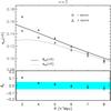Fig. 3 Effect of redshift-space distortions on the measurement and modelling of the clustering ratio. The values estimated in real and redshift space from the Lh halo catalogues (main panel) are compared with the theoretical predictions; these have been named and ηg,R respectively to indicate whether or not redshift-space distortions are included in the modelling. Each point represents the average over 31 mock catalogues (see text), while error bars give the corresponding standard deviation of the mean. The statistic is shown as a function of the filtering radius R and correlates the field on scales r = 3R. To obtain from Eq. (8) (solid line), we adopted a pairwise velocity dispersion σ12 = 200   km   s-1 (Bianchi et al. 2012; Marulli et al. 2012). The model accounts for both cases for non-linear evolution of the power spectrum by including the prescription of (Smith et al. 2003) into Eq. (2). The lower panel shows instead the relative difference between the LHS and left- and right-hand sides of Eq. (8) as a function of the same R. The shaded corridor indicates a ± 5% deviation.

Open with DEXTER

A typical assumption is that the non-linear distortion induced on the 2-point correlation function is driven by random motions and can be described as a convolution of the real-space correlation function with a Gaussian or Exponential kernel f(v₁₂) that describes the distribution of pairwise velocities along the line of sight (Davis & Peebles 1983) 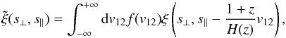(4)where s_∥ and s_⊥ are the separations along and perpendicular to the observer’s line of sight, H(z) is the Hubble parameter at redshift z, and 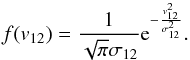With this definition note that the 1D Gaussian pairwise velocity dispersion σ₁₂ is times the dispersion in the pairwise velocity v₁₂ and it induces a dispersion in the radial comoving distance of amplitude σ_x = σ_v(1 + z)/H(z), where σ_v = σ₁₂/2 is the dispersion of galaxy peculiar velocities. Interestingly, this kernel has also been shown to model quasi-linear redshift-space effects (Percival & White 2009). This model can be straightforwardly re-mapped to Fourier space (Peacock & Dodds 1994), where the global (linear coherent + non-linear random) redshift-space distortions can be expressed as 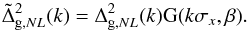In this expression, and give the (non-linear) power spectrum in redshift and real space, respectively, and (5)with β = f/b as the usual redshift space distortion parameter defined as the ratio between the linear growth rate and the linear bias parameter. Since we are essentially interested on scales, where y < 1, we can expand Eq. (5) as (6)where, K is the familiar Kaiser correction factor, while the even coefficients B_2n ~ 1 in the limit β < 1. Under these conditions, (7)With this approximation and G computed from Eq. (5), we can predict with sufficient accuracy the non-linear amplitude of η in redshift space, Interestingly, both the linear bias parameter and the scale-independent Kaiser correction have dropped out of this expression with the above “derivation” isolating the leading order contribution in G(y,β) and at the same time, decoupling the Kaiser model from the random dispersion. For a realistic value of β (≃0.5), assuming σ_v = 175   km   s^-1 and considering the scale R = 5   h^-1   Mpc, the approximation (8) is 1.6% at z = 1.

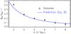	Fig. 4 Relative difference between the clustering ratio in real (ηg,R) and redshift () space. Black diamonds represent measurements from realistic galaxy mock catalogues characterized by a small scale velocity dispersion σ12 = 360 km s-1. The solid line shows predictions obtained by inserting this specific value σ12 into Eq. (8)
Open with DEXTER

Figure 3 shows how well Eq. (8) describes the actual behaviour of haloes in the L_h catalogues. For R = 4   h^-1   Mpc the relative discrepancy between theory and data is reduced from 14% to 4%, while for R = 5   h^-1   Mpc is as small as 2%. As discussed in Sect. 4.1, this level of systematic error (which is less than the statistical errors to be expected from VIPERS) is expected from the limitations of the adopted phenomenological description of the non-linear power spectrum in Eq. (8) (Smith et al. 2003) or from a possible non-local nature of galaxy bias at small R. The accuracy achieved with this simple model over the wide range of filtering scales R is remarkable, especially because it is not the result of fine-tuning the pairwise dispersion σ₁₂. In Fig. 3, the value was fixed to the value σ₁₂ = 200   km   s^-1 as measured from a dark matter simulation with similar mass resolution (Bianchi et al. 2012; Marulli et al. 2012). Such a low value for σ₁₂ is expected since haloes do not sample their own inner velocity dispersion. In Sect. 5.3, we discuss the robustness of Eq. (8) in more detail for a wider range of velocity dispersions. Notwithstanding, we show in Fig. 4 how well the simple model given in Eq. (8) accounts for small scale peculiar velocities in more realistic mock catalogues. To this purpose, we consider a galaxy sample obtained by populating haloes according to the halo occupation distribution (HOD) method. In Sect. 5.1 of de la Torre et al. (2013), they describe step by step how they obtained these mock catalogues from the MultiDark simulation (see Prada et al. 2012).

These results motivate our choice of R = 5   h^-1   Mpc as a smoothing scale for the analysis of the VIPERS data, since it maximises both the accuracy (minimizing the distance between data and theory, see Fig. 3) and the statistical precision of the estimate of η.

Fig. 5 Testing the sensitivity of η to the bias of the adopted tracers. Clustering statistics are estimated from two sub sets of the halo simulated catalogues, known as mid and low sub-samples tant include haloes with masses limited to M < 1013   h-1 M⊙ and M < 1012   h-1 M⊙, respectively. The left and right panels show the relative variation in the variance (upper), correlation function δξ ≡ ξg,R/ξg, R, ref − 1 (central), and clustering ratio δη ≡ ηg,R/ηg, R, ref − 1 with respect to the measurements from the full mock catalogues that contain all haloes with masses up to M = 7 × 1014   h-1 M⊙ for these two catalogues. In the left panel, quantities are measured from the Bh halo catalogues in real space, while the measurements on the right are performed in redshift space using the Lh light-cones. Error bars are estimated using the dispersion among the mock catalogues. For the sake of clarity, a relative shift along the abscissa is applied to the data in the bottom plots.

Open with DEXTER

4.3. Sensitivity to galaxy bias

In the linear regime, Eq. (8) is independent of galaxy biasing, where the clustering ratio does not depend on the particular tracer we use to estimate it. This is clearly only an approximation when non-linear scales are included. Evidence of the inadequacy of the hypothesis of locality, where a scale-dependence of galaxy bias (), emerges naturally on small scales. Similarly, the approximated redshift-space relation (8) explicitly neglects high order β contributions. We now establish the scales where the η statistics remains independent of the choice of the galaxy tracer.

The effects of scale-dependent bias are mitigated by the very definition of the η statistic as a ratio. For example, let’s consider the biasing model with parameters A = 1.7 and Q = 9.6 (Cole et al 2005). The relative variation db²/b² is as high as 32% in the interval 0.01 < k(h/Mpc)< 1, but results in η_R(r) change by less then 7%. Indeed, the clustering ratio on scales (R,r) = (5,15)   h^-1 Mpc roughly measures the relative strength of the power spectra at k_j0 ~ 0.09   h/Mpc and k_W ~ 0.3   h /Mpc, as shown by BM13 (see Sect. 3 of that paper), and, as a consequence, it is only sensitive to the variation in the bias between these two scales. Although useful in appreciating the favourable properties of the η statistic, this simple argument is clearly insufficient to quantify the impact of scale-dependent bias of VIPERS data on η. Analysing galaxy simulations is a more effective way to estimate the amplitude of the remaining systematic error.

We use the B_h (in real space) and L_h (in redshift space) simulated catalogues at z = 1, which contain haloes with masses up to M = 7 × 10¹⁴   h^-1   M_⊙. From these, we select two sub-samples that, have a lower bias compared to the full parent catalogues, by construction. We call these mid and low samples and include, respectively, only haloes with masses M < 10¹³   h^-1   M_⊙ and M < 10¹²   h^-1   M_⊙. The variance and 2-point correlation function of the smoothed density contrast δ_R from these samples are plotted in the upper and middle panels of Fig. 5, as a function of R. These are expressed in terms of their relative difference with respect to the full parent catalogues. The different bias of the two samples is evident on both local and non-local scales, as probed respectively by the two statistics σ_g,R and ξ_g,R. As predicted by theory, the lower panel confirms that, both quantities are biased in similar ways, such that the clustering ratio is essentially insensitive to this: systematic errors are limited to less than 1% (3%) in real (redshift) space with this choice of the mass threshold.

A further indication of the limited impact of a scale-dependent bias on the estimate of η_R from the VIPERS data is provided by a parallel analysis of the data themselves. Marulli et al. (2013) and de la Torre et al. (2013) measure the dependence of the galaxy correlation function on galaxy luminosity. The presence of any differential scale-dependent bias between samples with different luminosities would make us wary of non-local biasing effects entering in the clustering ratio as well. To investigate this, we consider the halo occupation distribution model fits to the measured VIPERS two-point correlations for five samples at ⟨ z ⟩  = 0.8 and luminosity between M_B < −22 and −20 (de la Torre et al. 2013, Fig. 12). Figure 6 shows HOD model power spectra corresponding to the best-fit HOD parameters for these samples. The plot shows that the shapes of the power spectra all follow the HALOFIT prescription, and only begin to diverge at k > 1   h /Mpc, or on scales to which η_R has little sensitivity. A luminosity-dependent scale-independent bias model therefore provides an excellent match to the data. The clustering ratio is sensitive to the power spectrum over two scales probed by the smoothed correlation function and the variance: Ŵ²(kR)j₀(nkR) and Ŵ²(kR). The range of wavenumbers that affect the ratio is determined by the broader top hat kernel Ŵ²(kR) with effective width k_max ~ π/R. From this argument, we see that the clustering ratio is mainly determined by the power spectrum at k < 0.6   h   Mpc^-1 for R = 5, thus by significantly smaller k’s than indicated by the tests of Fig. 6. This is explicitly shown by the right panel of the same figure, where η_R(3R) is computed as a function of R for the VIPERS galaxy samples. At R = 5   h^-1   Mpc, the difference between the Halofit prediction and the values estimated for the VIPERS samples differ by no more than 2%. Given the ~10% random errors expected on the estimates of η from the current PDR-1 VIPERS sample (Sect. 6), this shows that any systematic effect due to scale dependence of galaxy bias is expected to be negligible.

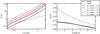Fig. 6 Left:best-fitting galaxy power spectra given the halo occupation distribution model fits for VIPERS galaxies in de la Torre et al. (2013). We examine five luminosity thresholded samples from MB < −22.0 to MB < −20 at z = 0.8. The HALOFIT matter power spectrum (black curve) and linear power spectrum (dashed curve) are overplotted. The galaxy power spectra are consistent with a luminosity-dependent constant bias model with respect to HALOFIT up to k = 1   h /Mpc. Right: values for the clustering ratio ηR(3R) are computed for the VIPERS galaxy power spectra. We find an agreement with the HALOFIT prediction at the 2% level at all scales down to R = 4   h-1 Mpc.

Open with DEXTER

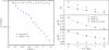Fig. 7 Left: radial number density of galaxies in the simulated W4 field before (diamonds) and after (triangles) implementing the radial selection function of VIPERS PDR-1. Right: estimations of the variance σg,R (upper), correlation function ξg,R(3R) (centre), and clustering ratio ηg,R(3R) (lower) from the true population of galaxies in the W4 field (diamonds) and from the sub-sample with the same VIPERS radial density profile (triangles) are shown as a function of the filtering scale R. Squares show estimates obtained after correcting the relevant statistical quantities for shot noise, using the local Poisson model (Layser 1956).

Open with DEXTER

5. The impact of observational effects on η

In this section, we discuss how observational effects have been accounted for in our analysis, and we test the robustness and limitations in producing an unbiased estimate of η from the VIPERS data.

For this, we use simulated galaxy samples that implement the VIPERS selection effects. We construct artificial galaxy light cones (named L_g hereafter) by populating the L_h simulations with a specific Halo Occupation Distribution (HOD) prescription, which are calibrated using VIPERS observations (de la Torre et al. 2013). The next step in obtaining fully realistic VIPERS mocks is to add the detailed survey selection function. The procedure that we follow is the same discussed in de la Torre et al. (2013): we first apply the magnitude cut i_AB < 22.5, then compute the observed redshift by incorporating the peculiar velocity contribution and a random component that reproduces the VIPERS redshift error distribution. We then add the effect of the colour selection on the radial distribution of the mocks. The latter is obtained by depleting the mocks at z < 0.6, so as to reproduce the Colour Sampling Rate (CSR, see Paper I). The mock catalogues that we obtain are then similar to the VIPERS parent photometric sample. We next apply the slit-positioning algorithm (SPOC, Bottini et al. 2005) with the same setting as for the data. This allows us to reproduce the VIPERS footprint on the sky; the small-scale angular incompleteness is due to spectra collisions and the variation in Target Sampling Rate across the fields. Finally, we deplete each quadrant to reproduce the effect of the Survey Success Rate (SSR). In this way, we end up with a set of 31 and 26 realistic mock catalogues (named L_gV hereafter), which simulate the detailed survey completeness function and observational biases of VIPERS in the W4 and W1 fields, respectively.

It is important to remark that the parent mock galaxy catalogues used here are not precisely the “standard” ones created for VIPERS or those discussed in de la Torre et al. (2013). In the latter, the mass resolution of the original L_h halo catalogues was improved by artificially adding low mass haloes following the prescriptions of de la Torre & Peacock (2013). This method uses the initial halo density field estimated on a regular grid, where the size is set by the mass resolution of the dark matter simulation. For the purpose of extending the halo mass range in the MultiDark simulation and creating VIPERS mock galaxy catalogues, an optimal grid size of 2.5   h^-1 Mpc has been chosen. However, as shown in de la Torre & Peacock (2013), the grid size, or reconstruction scale λ, can have some impact on the accuracy with which galaxy two-point correlations are reproduced. In particular, values of λ larger than the typical halo-halo separation, which are about 1   h^-1 Mpc, can lead to an underestimation of the two-point correlation function of galaxies that populate the reconstructed haloes. In de la Torre & Peacock (2013), they showed that the two-point correlation function on scales around 1   h^-1 Mpc is underestimated by few percents for the faintest galaxies for the adopted reconstruction scale used to create the standard VIPERS mocks. We found that the variance of the smoothed galaxy field measured in the standard mocks is also affected by this effect. For this reason and without loss of generality, we thus decided to use the L_g mock catalogues without the galaxies residing in the reconstructed haloes. Because these galaxies are hosted by haloes, which are systematically more massive than those hosting real VIPERS galaxies, does not affect the amplitude of the clustering ratio, which, as discussed in Sect. 4.3, is independent of the specific mass tracer.

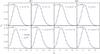Fig. 8 PDF of the number count overdensities δN within spheres of radius R = 5   h-1 Mpc (histograms) are measured from mock surveys that reproduce the full selection functions of the VIPERS W1 and W4 fields (left and right groups of four panels). This is compared with a reference sample drawn from the Poissonian PDF shown by the dashed lines. The four panels of each VIPERS field correspond to the PDF that one obtains when rejecting an increasingly larger number of cells, which depends on whether the fraction of the cells volume affected by the survey mask is smaller than the threshold wth indicated in the insets. The effect of “corrupted” cells is stronger in the W1 field, where it is necessary to reject all cells for which more than 40% of the volume is affected by the survey mask to recover the correct PDF. Error bars are obtained as the standard deviation over 50 distinct random catalogues. In the inset, we also quote the significance level of the Kolmogorov-Smirnov test on the agreement of the two distributions.

Open with DEXTER

5.1. Effects related to the radial selection function: shot noise

One effect of the selection function in a flux-limited sample is the increase in the shot noise as a function of distance due to the corresponding decrease of the mean density. One could correct for this by increasing the size of the smoothing window R, but this would remove the ability to compare fluctuations on the same scale at different redshifts. Rather, we assume that the data represents a local Poisson sampling of the underlying continuous density field and correct for this statistically (Layser 1956) and verify the limits of this assumption using our mock samples.

The right panel of Fig. 7 shows the effect of the shot noise correction on the two-point correlation function, the variance, and the clustering ratio. While the two-point function is insensitive to shot noise by construction, the variance does need to be corrected for the increasing Poisson noise, which is given by the inverse of the average counts in the spherical cells . When subtracted from the observed value, the effect is completely removed (square symbols).

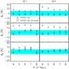Fig. 9 Testing the effectiveness of our correction for the VIPERS angular selection function on the clustering ratio η. From top to bottom, we show (for a smoothing radius R = 5   h-1 Mpc) the impact on the variance, 2-point correlation function, and clustering ratio ηg,R(3R). In each panel, we plot the mean and scatter over the mock samples of the relative difference δ between the “observed” and “true” quantities (multiplied by 100): triangles are for no correction at all, while squares corresponds to measurements using the correction method discussed in the text. The cyan shaded area correspond to a relative deviation smaller than ± 5%. Left and right panels correspond to W1 and W4, respectively.

Open with DEXTER

5.2. Effects related to the angular selection function

The VIPERS redshifts are being collected by tiling the selected sky areas with a uniform mosaic of VIMOS fields. The area covered is not contiguous but presents regular gaps due to the specific footprint of the instrument field of view, as well as to intrinsic unobserved areas due to bright stars or defects in the original photometric catalogue. The VIMOS field of view has four rectangular regions of about 8 × 7 square arcminutes each, which are separated by an unobserved cross (Guzzo et al. 2013; de la Torre et al. 2013). This creates a regular pattern of gaps in the angular distribution of the measured galaxies, which is clearly visible in Fig. 1. Additionally, the Target Sampling Rate and the Survey Success Rate vary among the quadrants, and a few of the latter were lost because of mechanical problems within VIMOS (see Paper I for details). Finally, the slit-positioning algorithm, SPOC, also introduces some small-scale angular selection effects with different constraints along the dispersion and spatial directions of the spectra, as thoroughly discussed in de la Torre et al. (2013). Clearly, this combination of angular selection effects has to be taken properly into account when estimating any clustering statistics.

In our specific case, this issue has been addressed as follows. We simulate a random (Poissonian) distribution of galaxies (hereafter called “parent catalogue”) and apply the global VIPERS angular selection function, which results from the combination of the photometric and spectroscopic masks, the TSR and the SSR.

We test whether the distributions of counts within cells of radius R match the expected Poisson distribution in Fig. 8 using the “parent” L_g (dashed line) and “observed” L_gV (histograms) mocks discussed earlier on. When the probability distribution function (PDF) is reconstructed using all possible cells that can be accommodated within the rectangular footprint of the W1 and W4 fields, the result is severely biased, which indicates that the sampling of the underlying PDF is not random. It is clear that gaps and holes lead to a broadening of the PDF, which is artificially skewed towards low counts and an overestimate of the power in 1- and 2-point statistics. We have demonstrated (Bel et al., in prep.) that this effect is mainly due to the missing full quadrants with a negligible contribution of the smaller gaps produced by the VIMOS footprint, or of the small-scale biases of the SPOC slit-positioning scheme. We also see that the effects are almost independent of the scale R used to compute the clustering statistics within the range explored here (3–8   h   Mpc^-1).

Bel et al. (in prep.) introduce a method to correct for such angular selection effects and recover the correct shape of the PDF and the corresponding moments to all orders. Here, we briefly summarize how we obtained a correct estimate of the variance, which we need for building the clustering ratio. As shown by Fig. 8, the size of the VIPERS PDR-1 sample is such that we can simply reject all spherical cells for which more 40% of the volume is affected by the overall survey mask, which corresponds to regions not covered by the survey. With this threshold, we recover the random sampling regime. Accordingly, we shall reject all the “seeds” for which at least one sphere of the surrounding motif does not satisfy the inclusion condition (see Sect. 3.2) in the computation of the two-point function. Once this selection process is applied, the underlying statistical properties of galaxies are properly reconstructed without any additional de-biasing procedure. The net result on the estimated statistics from the mocks is shown in Fig. 9. The three panels show that the variance, two-point correlation function, and clustering ratio for the “observed” L_gV mocks converge to the “true” value from the parent L_g. Independent of the correction, it is interesting to remark how, η is fairly insensitive to these effects. This happens because η is defined as the ratio of two quantities that are similarly affected. This is particularly impressive in the case of the W4 field, where η is virtually exact even without the correction. The price paid for this increased accuracy is clearly a larger statistical error on η due to the smaller effective survey volume.

5.3. Impact of redshift errors

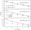Fig. 10 Clustering ratio ηg,R estimated from Lh haloes in real space (diamonds) is shown as a function of the filtering radius R and of the correlation length r = 3R. We also plot the clustering ratio estimated after perturbing the cosmological redshift of haloes with random errors (triangles). These random velocities are drawn from a Gaussian distribution with standard deviation σcz = (1 + z)σu km s-1 with σu as indicated. Also shown is the theoretically predicted value of obtained by inserting into Eq. (8) the corresponding value of σu. The points and error bars correspond to the average and standard deviation of the mean of the measurements over 31Lh catalogues. Such error bars, in practice, would correspond to the typical uncertainty in a survey with 31 times larger volume and 10 times higher galaxy number density than the VIPERS W4 sample.

Open with DEXTER

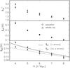Fig. 11 Impact and handling of the VIPERS redshift measurement errors on the usual statistical quantities that enter the definition of η, as plotted as a function of the filtering scale R and tested using the Lg mock catalogues. Triangles correspond to measurements performed after adding a redshift error randomly drawn from a Gaussian distribution with standard deviation σcz = 141(1 + z) to each galaxy position, which is representative of the errors affecting VIPERS redshifts (Guzzo et al. 2013). Diamonds give the reference values and are computed in redshift space without measurement errors. The dotted and solid lines give the clustering ratio predicted by Eq. (8) when a dispersion σv = 100   km   s-1 or (i.e. adding in quadrature the expected redshift error) are used, respectively. Expectation values and error bars are computed from the mocks in the usual way.

Open with DEXTER

Using repeated observations of 1215 objects in the the PDR-1 catalogue, the rms measurement error of VIPERS redshifts has been estimated to be σ_z = 0.00047(1 + z) or σ_cz = 141(1 + z) km s^-1 (see Paper I). At z ~ 1, this translates into an error in the radial comoving distance of ~3   h^-1 Mpc, which is expected in principle to have an impact on counts-in-cell statistics, for comparable cell sizes R.

The net effect of redshift errors is to smooth the galaxy distribution in redshift-space along the radial direction, suppressing the amplitude of 1-point statistics. This is similar to the effect of small-scale random peculiar velocities (although the latter on small scales are better described by an exponential distribution rather than a Gaussian). We therefore model the effect of redshift errors in the expression of η (Eq. (8)) by using an effective dispersion in the Gaussian damping term, or by adding in quadrature the VIPERS rms redshift error to the peculiar velocity dispersion of galaxies. We test the goodness of this description using the L_g mock surveys as described earlier, to which we add a radial displacement drawn from a Gaussian distribution with the appropriate dispersion. The results of measuring the variance , two-point correlation function , and clustering ratio of the smoothed field on the perturbed and unperturbed mocks, as compared to the corrected and uncorrected model, are shown in Fig. 11. As expected, the figure shows that, as expected, the amplitude of the effect (an underestimate of and an overestimate of ) increases for a decreasing smoothing scale R, when the latter becomes comparable to the redshift errors. To test the correction, we have estimated η_g,R in the L_h light cones of haloes in real space after having introduced random errors, which are characterised by the dispersion parameter σ_u (σ_cz = σ_u(1 + z)), in the cosmological redshift. The outcome of this analysis is presented in Fig. 10 and shows that Eq. (8) allows us to account for either small scale peculiar velocities or redshift errors.

5.4. Combined correction of systematic effects

We finally want to compare how well the combination of the different pieces we have developed and implemented into our description to account for non-linear and observational biases is capable of recovering the correct original value of η. This test is performed by comparing the “idealized” L_h mock surveys, which contain a population of dark matter haloes with constant density (no selection function, no mask) within the volume of the VIPERS survey, and the set of L_gV mocks, which contain HOD simulated galaxies that are selected according to the VIPERS selection function. We want to test whether the clustering ratio reconstructed from the VIPERS-like samples of galaxies after the correction for all the survey selection functions traces the clustering ratio reconstructed from the L_h samples. In other words, we want to determine if the clustering ratio is in agreement with catalogues characterized by a different set of tracers (haloes) masses (in the range 3 × 10¹¹ < M   h^-1   M_⊙ < 7 × 10¹⁴) without any VIPERS observational selection function (except from random redshift errors that we add to the haloes according to the techniques explained in Sect. 5.3).

The results of this analysis, as shown in Fig. 12, confirm the robustness of the clustering ratio. The same figure also shows the separate impact of the different effects and how η is particularly insensitive to some of them, due to its definition, as already shown in the previous sections. Specifically, these are all those biases that affect 1- and 2-point clustering statistics in the same sense.

6. Cosmological constraints from the VIPERS PDR-1 data

Using the methodology developed and tested in the previous sections, we are now in the position to apply the clustering ratio test to the VIPERS survey and study how well we can constrain the values of (at least some) cosmological parameters using the current catalogue.

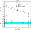Fig. 12 Overall impact and treatment of VIPERS selection effects on the estimate of the galaxy clustering ratio as a function of the smoothing scale R and for a correlation scale n = 3. The reference values of as measured in redshift space from the Lh halo catalogues (diamonds) are compared with those estimated from the realistic VIPERS-like mock samples LgV which include the radial and angular selection functions. The weight of the different corrections is determined by the different sets of points, as indicated in the legend. As usual, the plotted points represent ensemble averages over the mocks. Error bars on the reference Lh measurements (triangles) correspond to the standard deviation of the mean, while errors from the simulated VIPERS mocks give a forecast of the actual errors expected from the VIPERS data analysed in this paper (including cosmic variance). The solid line gives the theoretically predicted value of the clustering ratio from Eq. (8), including a pairwise velocity dispersion of σ12 = 200   km   s-1 (a plausible value, given the resolution of the simulation used see Bianchi et al. 2012; Marulli et al. 2012) and the rms error of the VIPERS redshifts (Guzzo et al. 2013). Note that this theoretical prediction is given as reference and is not the best fit model, as given the data.

Open with DEXTER

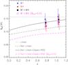Fig. 13 Galaxy clustering ratio on a scale of R = 5   h-1 Mpc and a correlation length n = 3, as estimated from real VIPERS data (squares) in two distinct redshift bins. Measurements for the individual VIPERS fields W1 (diamonds) and W4 (triangle) are also shown. The best fit theoretical model (cf. Eq. (8)) accounting for all non-linear and observational effects is given by the solid line. For comparison, we also display the corresponding linear theory prediction (dotted line) for the best fit cosmological parameters and the non-linear prediction when the corrections for peculiar motions and redshift errors are not included (short-dashed line). Error bars have been estimated from the standard deviation among the 31(/ 26)LgV mock VIPERS surveys of the W1/W4 fields, which include the contribution from cosmic variance. We also plot the observed and predicted values of when a “wrong” cosmology with slightly higher matter density Ωm0 = 0.4 is assumed (open squares and long-dashed curve, respectively). The divergence of observations and theory shows that this is not the best-fitting model, resulting in a low likelihood. For clarity, all data points have been slightly shifted along the abscissa.

Open with DEXTER

6.1. Likelihood definition

Let us first illustrate the procedure to evaluate P(p | η_g,R), which has the likelihood of the unknown set of parameters p = (Ω_m,Ω_X,w,H₀,Ω_bh²,n_s,σ₈,σ₁₂), given the observed value of η_g,R. The probability distribution function of the clustering ratio is not immediately obvious since this observable is defined via a ratio of two non-independent random variables. By using both simulated and real data, BM13 showed that the PDF of η_g,R is very well described by a Gaussian function, meaning that we can apply a standard χ² analysis.

In the analysis of the VIPERS sample we have considered two cases:

• a single redshift bin in the interval 0.65 < z < 1.2 (i.e. N = 1 in Eq. (8));

• two uncorrelated bins, at 0.65 < z < 0.93 and 0.93 < z < 1.2, i.e. with N = 2 in Eq. (8) (see Fig. 13).

In the following, we shall take their mean redshift as centres of these two bins rather than the median of the galaxy distribution. This choice is justified by the fact that this is approximately the redshift at which the accuracy in the estimate of η, as determined by the tradeoff between a decreasing number of objects and an increasing number of cells, has its peak. Note that this choice has no effect on the cosmological results.

In our analysis, we assume a flat cosmology in which the accelerated expansion is caused by a cosmological constant term in Einstein’s field equations (i.e., we fix the dark energy equation of state parameter to w = −1). As in BM13, we assume Gaussian priors on the baryonic matter density parameter Ω_bh² = 0.0213 ± 0.0010, the Hubble constant H₀ = 73.8 ± 2.4   km   s^-1Mpc^-1 and the primordial index n_s = 0.96 ± 0.014, as provided respectively by BBN (Pettini et al. 2008), HST (Riess et al. 2011) and WMAP7 (Larson et al. 2011) determinations. Additionally, we assume Gaussian priors on σ₈, which is re-parameterized as Δ_R(k_wmap)² = (2.208 ± 0.078) × 10^-9 with k_wmap = 0.027 Mpc^-1 (Komatsu et al. 2011) and on the effective pairwise velocity dispersion (σ₁₂ = 2σ_TOT = 514 ± 24   km   s^-1), as estimated from the VIPERS data themselves (priv. comm. by de la Torre). Finally, we underline that we do not include the full WMAP likelihood, which would introduce a strong prior on the matter density parameter Ω_mh².

The clustering ratio η_g,R(r,p) is estimated from the data by re-mapping the observed galaxy angular positions and redshifts into comoving distances, which vary the cosmology on a grid in a 6D space (Ω_m, H₀, Ω_bh², n_s, σ₈, σ₁₂). A consequence of this is that the posterior ℒ does not vary smoothly among the different models because the number of galaxies counted in any given cell that varies from model to model. However, the computation of the observable η_g,R(3R,p) is rather fast, given the counts-in-cells nature of the method. Therefore, shot noise is the price we have decided to pay in order to avoid fixing cosmological parameters at fiducial values and to obtain an unbiased likelihood hyper-surface.

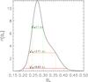	Fig. 14 Normalized 1D posterior probability of the density parameter at the current epoch, Ωm, estimated from the full VIPERS sample that is centred at z = 0.93. The curve is obtained by marginalizing the posterior over the remaining p parameters. The vertical dotted lines define the confidence intervals that correspond to , and .
Open with DEXTER

6.2. Results

In Fig. 13, we show the values of measured from the VIPERS data for (R,n) = (5   h^-1 Mpc,3), which splits the survey in different fashions (points). Note how the scatter between the estimates obtained by analysing the two fields W1 and W4 separately is compatible with the error bars that are estimated from the mock samples, suggesting that cosmic variance largely dominates the error budget. The curves correspond to the model (cf. Eq. (8)), which is computed for the best fit values of the parameters, as obtained for the whole survey. The solid line corresponds to the full model, which accounts for all non-linear corrections, whereas the dotted line gives the expected redshift-independent behaviour if η were measured (with the same derived parameters) on fully linear scales (for larger R as, for example, in BM13). The short-dashed line corresponds instead to only correcting for non-linear clustering but not for redshift-space distortions, while the magenta long-dashed line demonstrates the intrinsic sensitivity to Ω_m, which is further discussed in the following section (Sect. 6.3).

The best fit parameters have been first estimated splitting the data into two redshift bins (0.65 ≤ z < 0.93 and 0.93 < z ≤ 1.2). For these two volumes, the likelihood analysis yields and , respectively. Noticeably, error bars are smaller in the high redshift bin, despite the lower number density of galaxies. This is mainly the result of the 30% larger total volume but also of the smaller fraction of rejected cells in the process of mask correction. When the full redshift range 0.65 < z ≤ 1.2 is analysed at once, we obtain , which is the value used to produce the model curves in Fig. 13.

Figure 14 shows the 1D normalized posterior probability of Ω_m for this case, which is obtained by marginalizing P(p,η_g,R) over the remaining p elements. It is also interesting to note that if each element of the vector p = (Ω_m,H₀,Ω_bh²,n_s,σ₈,σ₁₂) is perturbed by + 10%, the corresponding variation induced in the amplitude of the clustering ratio is (−8.5%, −14.6%, 2.7%, 12%, 3%, 3%). This shows the specific sensitivity of η to the values of Ω_m, h, and n_s, as well as its weak dependence on Ω_bh², σ₈ and σ₁₂. The latter is particularly relevant, as the last two parameters enter into play here only because η is pushed to non-linear scales. The indication is therefore, once again, that the dependence on these specific parameters is weak. By giving a −40% change to the assumed central value of the Gaussian prior on the peculiar velocity dispersion σ_v, we change the estimated value of the matter density parameter by only −7%. This however remains as the biggest potential systematic in our analysis.

For comparison, the η-test to LRG galaxies of the SDSS DR7 sample is applied and (but smoothing the field on larger, more linear scales using R = 14   h^-1 Mpc), BM13 obtain Ω_m = 0.275 ± 0.020. This value is compared to those obtained here in Fig. 15. The roughly comparable uncertainty of the VIPERS and SDSS measurements, despite the smaller volume and number of objects of VIPERS, is explained by the much larger number of cells available to compute the statistic, when the field is smoothed on scales R = 5   h^-1 Mpc, as for VIPERS, rather than on 14  h^-1 Mpc, as used in the SDSS analysis of BM13. The price to be paid in the former case is that of having to handle and model non-linear scales.

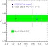Fig. 15 Value of the matter density parameter Ωm as estimated at different redshifts from the SDSS DR7 (Bel & Marinoni 2014) and VIPERS samples; the full sample (blue square) and two non-overlapping redshift bins (grey filled circles) correspond to 0.65 ≤ z < 0.93 and 0.93 < z ≤ 1.2. Both analyses assume a flat ΛCDM model and the same priors on common parameters. The dotted line shows the best fitting value for Ωm, as obtained combining the SDSS and VIPERS measurements.

Open with DEXTER

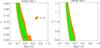Fig. 16 Left:two-dimensional marginalized constraints on Ωm,0 and H0 obtained by fitting the η measurements from VIPERS data with a flat ΛCDM model. Contours are plotted for ℒ−ℒmin < 2.3,6.17. In this case, Ωb   h2, ns, σ8, and σ12 are fixed to the value quoted in the text (i.e. they have a Dirac delta prior). We also draw curves corresponding to degeneracy along the loci Ωm,0h2 = const. (dotted line) and Ωm,0h = const. (dashed line). Right: the same but in the plane [Ωm,0, ns].

Open with DEXTER

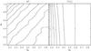Fig. 17 Sensitivity of the clustering ratio to the cosmological model, through left: isocontours of the function displaying the relative variation in the measured galaxy clustering ratio (with respect to the true cosmological model of the simulated data), which are induced by choosing a wrong cosmology in the redshift-distance conversion (i.e. a wrong guess of the cosmological parameters [Ωm,ΩX]). The redshift-space galaxy clustering ratio (left-hand side of Eq. (8)) is measured on scales (R,r) = (5,15)   h-1 Mpc from the stacking of the 31 Lh halo catalogues (which were built in a cosmology with Ωm = 0.27,ΩΛ = 0.73). The isocontours measure the strength of the Alcock-Paczynski geometric distortions, the deformation of the cell within which galaxies are counted. Right: the corresponding variation of the predicted mass clustering ratio (right-hand side of Eq. (8)) with varying cosmology. This panel evidences the sensitivity of η to Ωm through the shape of the transfer function.

Open with DEXTER

The excellent consistency of these measurements over a wide redshift interval (0 < z < 1.2) and from fully independent data sets is remarkable and strongly support the reliability of the measurements made by de la Torre et al. (2013). The combination of SDSS and VIPERS estimates of the matter density parameter gives Ω_m,0 = 0.274 ± 0.017, which improves the precision of the WMAP7 determination (Ω_m = 0.267 ± 0.029, Larson et al. 2011) by 75%, and by more than a factor of two when it is obtained by the joint analysis of the WMAP3 and SDSS DR5 data (Ω_m = 0.259 ± 0.039, Eisenstein et al. 2005). Our precision is comparable to that obtained by Percival et al. (2010; Ω_m = 0.278 ± 0.018) from the combination of BAO measurements from SDSS DR7 and 2dFRGS and the full WMAP5 likelihood (Dunkley et al. 2009). We also note that the most recent analyses of the BOSS data give Ω_m = 0.298 ± 0.017, when using BAO and WMAP7 (Anderson et al. 2012) and Ω_m0 = 0.282 ± 0.015 from the combination of the full correlation function with WMAP7 (Sanchez et al. 2012).

It is important to remark that our estimates of Ω_m using the observed values of η were obtained without including the full CMB likelihood, as this would have forced a very strong prior on Ω_mh². We did, however, include priors on the parameters H₀ and n_s on which the analysis is sensitive, as discussed earlier. The additional degrees of freedom arising when these two priors in the likelihood analysis are relaxed are shown in Fig. 16. At least for the range explored, the degeneracy axis in the (Ω_m,h) plane develops along the line Ω_mh² = const. This is different from measurements in the linear regime, where the degeneracy roughly follows an Ω_mh = const. locus. In principle, a redshift survey larger than (but as dense as) VIPERS could be able to simultaneously constrain Ω_m and h with a single probe by combining measurements of η with small and large smoothing scale R.

We also note that the VIPERS value is only ~7% smaller than the value we obtain from the L_gV mock catalogues in a ΛCDM cosmology. Given that the best fitting and the simulated cosmological models are extremely close, this agreement independently confirms that systematic errors are effectively taken care of.

6.3. Discussion: specific sensitivity of η to cosmological parameters

In Fig. 13, we provide an explicit example of how the η test works by plotting both the measurements (open squares) and the expectation of the full non-linear model (long-dashed line) when a different cosmology is adopted. In this case, Ω_m has been set to 0.4 within the same flat Λ model. The choice of a slightly wrong cosmology makes the data and the model incompatible. On one side, the distortion of the cosmological volume of the cell due to the calculation of distances results in a smaller measured value of . At the same time, the theoretical expectation is even lower due to the different shape of P(k) implied by the higher Ω_m.

In terms of specific cosmological parameters, the right-hand side of Eq. (8) depends on the shape of the matter power spectrum in real space. This means it is directly sensitive to the primordial index n_s and to the parameters determining the size of the horizon scale at matter-radiation equality¹, or Ω_mh² and Ω_bh². Since we pushed the analysis into the weakly non-linear regimes in this case, two additional parameters appear in the theoretical model (8) with respect to the linear analysis of BM13: the normalization of the power spectrum σ₈, which enters the expression of the shape of the quasi-linear power spectrum of Smith et al. (2003) and the galaxy pairwise velocity dispersion σ₁₂, which parameterizes the suppression of small-scale power produced by disordered peculiar velocities. The distance-redshift relation enters the left-hand side of Eq. (8) changing the volume and shape of each sphere and their relative distance in the directions parallel and perpendicular to the observer line’s of sight (Alcock-Paczynski effect). Together, these add some sensitivity to the density parameter, Ω_x, and equation of state, w, of dark energy.

It is interesting to discuss the relative contribution of the geometrical and power spectrum shape, which are shown and compared in Fig. 17. The geometric distortions in η_g,R(r) (for R = 5   h^-1 Mpc and r = 3R) are equally sensitive to both the dark matter and the dark energy densities as indicated by the degeneracy axes (i.e. the isocontours), which are tilted by ~45° in the [Ω_m,Ω_X] plane. The absolute amplitude of the distance-redshift translation, however, is weak. The clustering ratio varies from 10% to −20% around its true value (estimated in the true cosmology) when the matter density parameter goes from 0.2 to 0.8 as shown in Fig. 17. The mass clustering ratio is extremely sensitive to the matter density parameter Ω_m. A change by ~0.1(−0.1) of the true value (in this case Ω_m = 0.27) induces a change in η_R of ~−30%(+60%). Note also the extremely weak dependence of the isocontours on the dark energy parameter. This arises because we parameterize the local normalization σ₈ in terms of the seven-year WMAP normalization prior 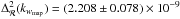, where k_wmap = 0.027 Mpc^-1 (Komatsu et al. 2011). Mapping the primordial (linear) curvature perturbations ℛ into the present day rms of the matter density fluctuations, σ₈, causes the non-linear power spectrum to acquire an extra sensitivity to the dark energy content (and to the gravitational model) of the universe.

In conclusion, we see that the cosmological signal measured by η from the VIPERS data is primarily encoded in the shape of the power spectrum rather than in space geometry. To obtain meaningful limits on Ω_v (or, more directly, the degree of matter domination at z ≃ 1), Fig. 17 indicates that it is necessary to measure Ω_m to a precision of better than about 5%. This is approximately the precision achieved in the current analysis, so it will be worth revisiting the geometrical aspect of the η test when the final VIPERS dataset is complete.

7. Summary

In this paper, we have applied the galaxy clustering ratio proposed by Bel & Marinoni (2014) to a sub set of the new VIPERS PDR-1 redshift catalogue which includes 26 611 galaxies. A large part of the paper has been dedicated to verifying the robustness of applying this statistics to mildly non-linear scales, where non-linear clustering, redshift-space distortions, and scale-dependence of biasing need to be accounted for.

Ideally, η_g,R(r) should be estimated in the linear regime (large R and r values), where its amplitude is theoretically predicted in a straightforward way. Nonetheless, we have shown that a simple, theoretically motivated modelling of the expected non-linear corrections is sufficient to preserve its value as a powerful cosmological probe also in the mildly non-linear regime in this paper. These corrections include: (a) the effect of random peculiar velocities, or non-linear redshift distortions on small scales: we have also shown that the effect of redshift errors can be incorporated within the same scheme once an effective pairwise dispersion is considered. (b) The scale dependence of bias: we have shown that this effect does not introduce a significant systematic error on the measurements of η for realistic dependences. This is not simply a question of assuming a mild dependence on scale of the bias but that its effect can be minimized by a careful choice of the scales of smoothing (R) and correlation (r) in terms of which η is defined.

Based on these results, we have used η to extract cosmological information from the new PDR-1 data of the VIPERS survey, which is limited to z > 0.65. We first split the sample into two redshift slices with a mean redshift z = 0.79 and z = 1.07. This exercise yielded two independent estimates of the matter density parameter at the current epoch, and , respectively. To obtain these estimates, we included external priors on Ω_bh²,h,n_s and , but not the strong one on Ω_mh² from WMAP. We also analysed the full redshift range 0.65 < z < 1.2 as a single sample, obtaining a value .

The two measurements of η from VIPERS with that from the SDSS by BM13 provide us with three independent estimates at three different cosmic epochs based on the same external priors. These allow us to: i) confirm the consistency of the standard ΛCDM cosmological model over a wide redshift baseline, covering almost half the age of the Universe; and ii) obtain a stronger constraint on the local value of Ω_m than allowed by the two redshift surveys alone (~7%), corresponding to a transition redshift between the matter and cosmological-constant dominated epochs of z_md = 0.395 ± 0.04.

It is interesting to compare these figures to those we previously obtained using the angular power spectrum of the full CFHTLS parent galaxy sample (sliced using the same VIPERS colour selection criteria), which are coupled to an earlier VIPERS catalogue (Granett et al. 2012). This sample, assuming flatness and letting the matter density as a free fitting parameter (with Dirac priors on all other relevant cosmological quantities), yielded Ω_m,0 = 0.30 ± 0.06.

The VIPERS measurement of Ω_m,0 is also consistent with the estimate obtained by BM13 using the same technique applied to the SDSS LRG sample at z ~ 0.3, Ω_m,0 = 0.275 ± 0.020. The combination of these two estimates of Ω_m,0, as obtained from data that cover the large range 0 < z < 1.2, gives a best value of Ω_m,0 = 0.274 ± 0.017. For comparison, the recent combination of the Planck TT power spectrum with WMAP polarization gives Ω_m,0 = 0.315 ± 0.017. Note that the apparent tension between those measurements is mainly due to the prior on H₀ coming from the HST measurements. Indeed, a lower value of H₀ would result in a larger matter density.

Acknowledgments

J.B. and C.M. acknowledge useful discussions with F. Bernardeau, E. Gaztañaga, and I. Szapudi. We thank the referee for well-directed comments. We acknowledge the crucial contribution of the ESO staff for the management of service observations. In particular, we are deeply grateful to M. Hilker for his constant help and support of this programme. Italian participation to VIPERS has been funded by INAF through PRIN 2008 and 2010 programmes. L.G. and B.J.G. acknowledges support of the European Research Council through the Darklight ERC Advanced Research Grant (# 291521). O.L.F. acknowledges support of the European Research Council through the EARLY ERC Advanced Research Grant (# 268107). Polish participants have been supported by the Polish Ministry of Science (grant N N203 51 29 38), the Polish-Swiss Astro Project (co-financed by a grant from Switzerland, through the Swiss Contribution to the enlarged European Union), the European Associated Laboratory Astrophysics Poland-France HECOLS and a Japan Society for the Promotion of Science (JSPS) Postdoctoral Fellowship for Foreign Researchers (P11802). G.D.L. acknowledges financial support from the European Research Council under the European Community’s Seventh Framework Programme (FP7/2007-2013)/ERC grant agreement No. 202781. W.J.P. and R.T. acknowledge financial support from the European Research Council under the European Community’s Seventh Framework Programme (FP7/2007-2013)/ERC grant agreement No. 202686. W.J.P. is also grateful for support from the UK Science and Technology Facilities Council through the grant ST/I001204/1. E.B., F.M. and L.M. acknowledge the support from grants ASI-INAF I/023/12/0 and PRIN MIUR 2010-2011. C.M. is grateful for support from specific project funding of the Institut Universitaire de France and the LABEX OCEVU.

References

All Figures

	Fig. 1 Distribution on the sky of the galaxies with measured redshifts in the VIPERS PDR-1 catalogue within the W1 and W4 fields (blue points). The pattern described by the gaps separating the VIMOS quadrants, as well as the areas not covered by the PDR-1, are clearly visible. Superimposed to the spectroscopic data, we also plot for illustrative purposes the projection of a subset of the spherical cells used to estimate the variance (regular grid on the left) with the typical motif used to estimate the 2-point correlation function of the smoothed density field ξg,R(r) (right). The spheres have a radius of R = 5   h-1   Mpc, and the chosen set is placed at redshift z = 0.66. Note that the distance between the centres of 2 opposite spheres in the motif is exactly equal to the chosen correlation scale r (we show here the case r = 3R). Red circles correspond to spheres that have been rejected in the clustering analysis because they are heavily affected by the survey mask (see discussion in Sect. 5.2.)
Open with DEXTER
In the text

	Fig. 2 Impact of non-linear clustering on the measurement and theoretical modelling of the galaxy clustering ratio η. The latter is measured in real space for the halo catalogues of the Bh simulation and compared to both the linear and non-linear predictions, as described respectively by a simple Eisenstein & Hu (1998) linear power spectrum (dot-dashed lines) and after correction through the non-linear HALOFIT prescription of Smith et al. (2003) (solid lines). The clustering ratio is shown as a function of the smoothing scale R adopted to filter the discrete distribution of haloes and for various correlation lengths (r = nR) with n =  { 2,3,4 }. Errors bars are obtained using 64 block-jackknife resampling of the data which excludes a cubic volume of linear size 250   h-1   Mpc each time.
Open with DEXTER
In the text

	Fig. 3 Effect of redshift-space distortions on the measurement and modelling of the clustering ratio. The values estimated in real and redshift space from the Lh halo catalogues (main panel) are compared with the theoretical predictions; these have been named and ηg,R respectively to indicate whether or not redshift-space distortions are included in the modelling. Each point represents the average over 31 mock catalogues (see text), while error bars give the corresponding standard deviation of the mean. The statistic is shown as a function of the filtering radius R and correlates the field on scales r = 3R. To obtain from Eq. (8) (solid line), we adopted a pairwise velocity dispersion σ12 = 200   km   s-1 (Bianchi et al. 2012; Marulli et al. 2012). The model accounts for both cases for non-linear evolution of the power spectrum by including the prescription of (Smith et al. 2003) into Eq. (2). The lower panel shows instead the relative difference between the LHS and left- and right-hand sides of Eq. (8) as a function of the same R. The shaded corridor indicates a ± 5% deviation.
Open with DEXTER
In the text

	Fig. 4 Relative difference between the clustering ratio in real (ηg,R) and redshift () space. Black diamonds represent measurements from realistic galaxy mock catalogues characterized by a small scale velocity dispersion σ12 = 360 km s-1. The solid line shows predictions obtained by inserting this specific value σ12 into Eq. (8)
Open with DEXTER
In the text

	Fig. 5 Testing the sensitivity of η to the bias of the adopted tracers. Clustering statistics are estimated from two sub sets of the halo simulated catalogues, known as mid and low sub-samples tant include haloes with masses limited to M < 1013   h-1 M⊙ and M < 1012   h-1 M⊙, respectively. The left and right panels show the relative variation in the variance (upper), correlation function δξ ≡ ξg,R/ξg, R, ref − 1 (central), and clustering ratio δη ≡ ηg,R/ηg, R, ref − 1 with respect to the measurements from the full mock catalogues that contain all haloes with masses up to M = 7 × 1014   h-1 M⊙ for these two catalogues. In the left panel, quantities are measured from the Bh halo catalogues in real space, while the measurements on the right are performed in redshift space using the Lh light-cones. Error bars are estimated using the dispersion among the mock catalogues. For the sake of clarity, a relative shift along the abscissa is applied to the data in the bottom plots.
Open with DEXTER
In the text

	Fig. 6 Left:best-fitting galaxy power spectra given the halo occupation distribution model fits for VIPERS galaxies in de la Torre et al. (2013). We examine five luminosity thresholded samples from MB < −22.0 to MB < −20 at z = 0.8. The HALOFIT matter power spectrum (black curve) and linear power spectrum (dashed curve) are overplotted. The galaxy power spectra are consistent with a luminosity-dependent constant bias model with respect to HALOFIT up to k = 1   h /Mpc. Right: values for the clustering ratio ηR(3R) are computed for the VIPERS galaxy power spectra. We find an agreement with the HALOFIT prediction at the 2% level at all scales down to R = 4   h-1 Mpc.
Open with DEXTER
In the text

	Fig. 7 Left: radial number density of galaxies in the simulated W4 field before (diamonds) and after (triangles) implementing the radial selection function of VIPERS PDR-1. Right: estimations of the variance σg,R (upper), correlation function ξg,R(3R) (centre), and clustering ratio ηg,R(3R) (lower) from the true population of galaxies in the W4 field (diamonds) and from the sub-sample with the same VIPERS radial density profile (triangles) are shown as a function of the filtering scale R. Squares show estimates obtained after correcting the relevant statistical quantities for shot noise, using the local Poisson model (Layser 1956).
Open with DEXTER
In the text

	Fig. 8 PDF of the number count overdensities δN within spheres of radius R = 5   h-1 Mpc (histograms) are measured from mock surveys that reproduce the full selection functions of the VIPERS W1 and W4 fields (left and right groups of four panels). This is compared with a reference sample drawn from the Poissonian PDF shown by the dashed lines. The four panels of each VIPERS field correspond to the PDF that one obtains when rejecting an increasingly larger number of cells, which depends on whether the fraction of the cells volume affected by the survey mask is smaller than the threshold wth indicated in the insets. The effect of “corrupted” cells is stronger in the W1 field, where it is necessary to reject all cells for which more than 40% of the volume is affected by the survey mask to recover the correct PDF. Error bars are obtained as the standard deviation over 50 distinct random catalogues. In the inset, we also quote the significance level of the Kolmogorov-Smirnov test on the agreement of the two distributions.
Open with DEXTER
In the text

	Fig. 9 Testing the effectiveness of our correction for the VIPERS angular selection function on the clustering ratio η. From top to bottom, we show (for a smoothing radius R = 5   h-1 Mpc) the impact on the variance, 2-point correlation function, and clustering ratio ηg,R(3R). In each panel, we plot the mean and scatter over the mock samples of the relative difference δ between the “observed” and “true” quantities (multiplied by 100): triangles are for no correction at all, while squares corresponds to measurements using the correction method discussed in the text. The cyan shaded area correspond to a relative deviation smaller than ± 5%. Left and right panels correspond to W1 and W4, respectively.
Open with DEXTER
In the text

	Fig. 10 Clustering ratio ηg,R estimated from Lh haloes in real space (diamonds) is shown as a function of the filtering radius R and of the correlation length r = 3R. We also plot the clustering ratio estimated after perturbing the cosmological redshift of haloes with random errors (triangles). These random velocities are drawn from a Gaussian distribution with standard deviation σcz = (1 + z)σu km s-1 with σu as indicated. Also shown is the theoretically predicted value of obtained by inserting into Eq. (8) the corresponding value of σu. The points and error bars correspond to the average and standard deviation of the mean of the measurements over 31Lh catalogues. Such error bars, in practice, would correspond to the typical uncertainty in a survey with 31 times larger volume and 10 times higher galaxy number density than the VIPERS W4 sample.
Open with DEXTER
In the text

	Fig. 11 Impact and handling of the VIPERS redshift measurement errors on the usual statistical quantities that enter the definition of η, as plotted as a function of the filtering scale R and tested using the Lg mock catalogues. Triangles correspond to measurements performed after adding a redshift error randomly drawn from a Gaussian distribution with standard deviation σcz = 141(1 + z) to each galaxy position, which is representative of the errors affecting VIPERS redshifts (Guzzo et al. 2013). Diamonds give the reference values and are computed in redshift space without measurement errors. The dotted and solid lines give the clustering ratio predicted by Eq. (8) when a dispersion σv = 100   km   s-1 or (i.e. adding in quadrature the expected redshift error) are used, respectively. Expectation values and error bars are computed from the mocks in the usual way.
Open with DEXTER
In the text

	Fig. 12 Overall impact and treatment of VIPERS selection effects on the estimate of the galaxy clustering ratio as a function of the smoothing scale R and for a correlation scale n = 3. The reference values of as measured in redshift space from the Lh halo catalogues (diamonds) are compared with those estimated from the realistic VIPERS-like mock samples LgV which include the radial and angular selection functions. The weight of the different corrections is determined by the different sets of points, as indicated in the legend. As usual, the plotted points represent ensemble averages over the mocks. Error bars on the reference Lh measurements (triangles) correspond to the standard deviation of the mean, while errors from the simulated VIPERS mocks give a forecast of the actual errors expected from the VIPERS data analysed in this paper (including cosmic variance). The solid line gives the theoretically predicted value of the clustering ratio from Eq. (8), including a pairwise velocity dispersion of σ12 = 200   km   s-1 (a plausible value, given the resolution of the simulation used see Bianchi et al. 2012; Marulli et al. 2012) and the rms error of the VIPERS redshifts (Guzzo et al. 2013). Note that this theoretical prediction is given as reference and is not the best fit model, as given the data.
Open with DEXTER
In the text

	Fig. 13 Galaxy clustering ratio on a scale of R = 5   h-1 Mpc and a correlation length n = 3, as estimated from real VIPERS data (squares) in two distinct redshift bins. Measurements for the individual VIPERS fields W1 (diamonds) and W4 (triangle) are also shown. The best fit theoretical model (cf. Eq. (8)) accounting for all non-linear and observational effects is given by the solid line. For comparison, we also display the corresponding linear theory prediction (dotted line) for the best fit cosmological parameters and the non-linear prediction when the corrections for peculiar motions and redshift errors are not included (short-dashed line). Error bars have been estimated from the standard deviation among the 31(/ 26)LgV mock VIPERS surveys of the W1/W4 fields, which include the contribution from cosmic variance. We also plot the observed and predicted values of when a “wrong” cosmology with slightly higher matter density Ωm0 = 0.4 is assumed (open squares and long-dashed curve, respectively). The divergence of observations and theory shows that this is not the best-fitting model, resulting in a low likelihood. For clarity, all data points have been slightly shifted along the abscissa.
Open with DEXTER
In the text

	Fig. 14 Normalized 1D posterior probability of the density parameter at the current epoch, Ωm, estimated from the full VIPERS sample that is centred at z = 0.93. The curve is obtained by marginalizing the posterior over the remaining p parameters. The vertical dotted lines define the confidence intervals that correspond to , and .
Open with DEXTER
In the text

	Fig. 15 Value of the matter density parameter Ωm as estimated at different redshifts from the SDSS DR7 (Bel & Marinoni 2014) and VIPERS samples; the full sample (blue square) and two non-overlapping redshift bins (grey filled circles) correspond to 0.65 ≤ z < 0.93 and 0.93 < z ≤ 1.2. Both analyses assume a flat ΛCDM model and the same priors on common parameters. The dotted line shows the best fitting value for Ωm, as obtained combining the SDSS and VIPERS measurements.
Open with DEXTER
In the text

	Fig. 16 Left:two-dimensional marginalized constraints on Ωm,0 and H0 obtained by fitting the η measurements from VIPERS data with a flat ΛCDM model. Contours are plotted for ℒ−ℒmin < 2.3,6.17. In this case, Ωb   h2, ns, σ8, and σ12 are fixed to the value quoted in the text (i.e. they have a Dirac delta prior). We also draw curves corresponding to degeneracy along the loci Ωm,0h2 = const. (dotted line) and Ωm,0h = const. (dashed line). Right: the same but in the plane [Ωm,0, ns].
Open with DEXTER
In the text

	Fig. 17 Sensitivity of the clustering ratio to the cosmological model, through left: isocontours of the function displaying the relative variation in the measured galaxy clustering ratio (with respect to the true cosmological model of the simulated data), which are induced by choosing a wrong cosmology in the redshift-distance conversion (i.e. a wrong guess of the cosmological parameters [Ωm,ΩX]). The redshift-space galaxy clustering ratio (left-hand side of Eq. (8)) is measured on scales (R,r) = (5,15)   h-1 Mpc from the stacking of the 31 Lh halo catalogues (which were built in a cosmology with Ωm = 0.27,ΩΛ = 0.73). The isocontours measure the strength of the Alcock-Paczynski geometric distortions, the deformation of the cell within which galaxies are counted. Right: the corresponding variation of the predicted mass clustering ratio (right-hand side of Eq. (8)) with varying cosmology. This panel evidences the sensitivity of η to Ωm through the shape of the transfer function.
Open with DEXTER
In the text

References

- Alcock, C., & Paczynski, B. 1979, Nature, 281, 358 [NASA ADS] [CrossRef] [Google Scholar]
- Amendola, L., Appleby, S., Bacon, D., et al. 2013, Liv. Rev. Relativ., 16, 6 [NASA ADS] [CrossRef] [Google Scholar]
- Anderson, L., Aubourg, E., Bailey, S., et al. 2012, MNRAS, 427, 3435 [Google Scholar]
- Ballinger, W. E., Peacock, J. A., & Heavens, A. F. 1996, MNRAS, 282, 877 [NASA ADS] [CrossRef] [Google Scholar]
- Bel, J., & Marinoni, C. 2012, MNRAS, 424, 971 [NASA ADS] [CrossRef] [Google Scholar]
- Bel, J., & Marinoni, C. 2014, A&A, 563, A36 [NASA ADS] [CrossRef] [EDP Sciences] [Google Scholar]
- Bianchi, D., Guzzo, L., Branchini, E., et al. 2012, MNRAS, 427, 2420 [NASA ADS] [CrossRef] [Google Scholar]
- Blake, C., Glazebrook, K., Davis, T. M., et al. 2011, MNRAS, 418, 1707 [NASA ADS] [CrossRef] [MathSciNet] [Google Scholar]
- Bottini, D., Garilli, B., Maccagni, D., et al. 2005, PASP, 117, 996 [NASA ADS] [CrossRef] [Google Scholar]
- Cole, S., Percival, W., & Peacock, J., et al. 2005, MNRAS, 362, 505 [NASA ADS] [CrossRef] [Google Scholar]
- Colless, M., Dalton, G., Maddox, S., et al. 2001, MNRAS, 328, 1039 [NASA ADS] [CrossRef] [Google Scholar]
- Cooray, A., & Sheth, R. 2002, Phys. Rep., 372, 1 [NASA ADS] [CrossRef] [Google Scholar]
- Dekel, A., & Lahav, O. 1999, ApJ, 520, 24 [NASA ADS] [CrossRef] [MathSciNet] [Google Scholar]
- de la Torre, S., & Peacock, J. 2013, MNRAS, 435, 743 [NASA ADS] [CrossRef] [Google Scholar]
- de la Torre, S., Guzzo, L., Kovac, K., et al. (the ZCOSMOS collaboration) 2010, MNRAS, 409, 867 [NASA ADS] [CrossRef] [Google Scholar]
- de la Torre, S., Guzzo, L., Peacock, J. A., et al. (VIPERS team) 2013, A&A, 557, A54 [NASA ADS] [CrossRef] [EDP Sciences] [Google Scholar]
- Drinkwater, M. J., Jurek, R. J., Blake, C., et al. 2010, MNRAS, 401, 1429 [Google Scholar]
- Dunkley, J., Spergel, D. N., Komatsu, E., et al. 2009, ApJS, 180, 306 [NASA ADS] [CrossRef] [Google Scholar]
- Eisenstein, D. J., & Hu, W. 1998, ApJ, 496, 605 [NASA ADS] [CrossRef] [Google Scholar]
- Eisenstein, D., Zehavi, I., Hogg, D. W., et al. 2005, ApJ, 633, 560 [NASA ADS] [CrossRef] [Google Scholar]
- Eisenstein, D. J., Weinberg, D. H., Agol, E., et al. 2011, AJ, 142, 72 [Google Scholar]
- Fry, J. N., & Gaztañaga, E. 1993, ApJ, 413, 447 [NASA ADS] [CrossRef] [Google Scholar]
- Gao, L., & White, S. D. M. 2007, MNRAS, 377, L5 [NASA ADS] [CrossRef] [Google Scholar]
- Garilli, B., Le Fèvre, O., Guzzo, L., et al. (the VVDS collaboration) 2008, A&A, 486, 683 [NASA ADS] [CrossRef] [EDP Sciences] [Google Scholar]
- Garilli, B., Paioro, L., Scodeggio, M., et al. 2012, PASP, 124, 1232 [NASA ADS] [CrossRef] [Google Scholar]
- Granett, B. R., Guzzo, L., Coupon, J., et al. 2012, MNRAS, 421, 251 [NASA ADS] [Google Scholar]
- Guzzo, L., Pierleoni, M., Meneux, B., et al. (the VVDS team) 2008, Nature, 451, 541 [NASA ADS] [CrossRef] [PubMed] [Google Scholar]
- Guzzo, L., Scodeggio, M., Garilli, B., et al. (the VIPERS team) 2013, A&A, submitted [arXiv:1303.2623] [Google Scholar]
- Heitmann, K., White, M., Wagner, C., Habib, S., & Higdon, D. 2010, ApJ, 715, 104 [NASA ADS] [CrossRef] [Google Scholar]
- Jackson, J. C. 1972, MNRAS, 156 [Google Scholar]
- Kaiser, N. 1984, ApJ, 284, 9 [Google Scholar]
- Kaiser, N. 1987, MNRAS, 227, 1 [NASA ADS] [CrossRef] [Google Scholar]
- Komatsu, E., Smith, K. M., Dunkley, J., et al. 2011, ApJS, 192, 18 [NASA ADS] [CrossRef] [Google Scholar]
- Kovac, K., Porciani, C., Lilly, S. J., et al. 2011, ApJ, 731, 102 [NASA ADS] [CrossRef] [Google Scholar]
- Kron, R. C. 1980, ApJ, 241, 25 [NASA ADS] [CrossRef] [Google Scholar]
- Larson, D., Dunkley, J., Hinshaw, G., et al. 2011, ApJS, 192, 16 [NASA ADS] [CrossRef] [Google Scholar]
- Laureijs, R., Amiaux, J., Arduini, S., et al. (the EUCLID collaboration) 2011 [arXiv:1110.3193] [Google Scholar]
- Layser, D. 1956, ApJ, 61, 1243 [Google Scholar]
- Le Fèvre, O., Prieto, E., & Posselt, W. 2000, ASPC, 207, 313L [NASA ADS] [Google Scholar]
- Le Fèvre, O., Saisse, M., Mancini, D., et al. 2003, Proc. SPIE, 4841, 1670 [NASA ADS] [CrossRef] [Google Scholar]
- Le Fèvre, O., Vettolani, G., Garilli, B., et al. 2005, A&A, 439, 845 [NASA ADS] [CrossRef] [EDP Sciences] [Google Scholar]
- Lilly, S. J., Le Brun, V., Maier, C., et al. (the ZCOSMOS collaboration) 2009, ApJS, 184, 218 [Google Scholar]
- Marchetti, A., Granett, B. R., Guzzo, L., et al. (the VIPERS team) 2013, MNRAS, 428, 1424 [NASA ADS] [CrossRef] [Google Scholar]
- Marinoni, C. & Buzzi, A. 2010, Nature, 468, 539 [NASA ADS] [CrossRef] [PubMed] [Google Scholar]
- Marinoni, C., Le Fèvre, O., Meneux, B., et al. 2005, A&A, 442, 801 [NASA ADS] [CrossRef] [EDP Sciences] [Google Scholar]
- Marinoni, C., Bel, J., & Buzzi, A. 2012, JCAP, 10, 36 [Google Scholar]
- Marulli, F., Bianchi, D., Branchini, E., et al. 2012, MNRAS, 426, 2566 [NASA ADS] [CrossRef] [Google Scholar]
- Marulli, F., Bolzonella, M., Branchini, E., et al. (the VIPERS team) 2013, A&A, 557, 17A [Google Scholar]
- Mellier, Y., Bertin, E., Hudelot, P., et al. 2008, The CFHTLS T0005 Release, http://terapix.iap.fr/cplt/oldSite/Descart/CFHTLS-T0005-Release.pdf [Google Scholar]
- Mo, H. J., & White, S. D. M. 1996, MNRAS, 282, 347 [NASA ADS] [CrossRef] [Google Scholar]
- Newman, J. A., Cooper, M. C., Davis, M., et al. (the DEEP2 collaboration) 2013, ApJS, 208, 5 [Google Scholar]
- Oke, J. B., & Gunn, J. E. 1983, ApJ, 266, 713 [NASA ADS] [CrossRef] [Google Scholar]
- Peacock, J. A. 1992, MNRAS, 258, 581 [NASA ADS] [Google Scholar]
- Peacock, J. A., & Dodds, S. J. 1994, MNRAS, 267, 1020 [NASA ADS] [Google Scholar]
- Peacock, J. A., Cole, S., Norberg, P., et al. 2001, Nature, 410, 169 [NASA ADS] [CrossRef] [PubMed] [Google Scholar]
- Percival, W. J., & White, M. 2009, MNRAS, 393, 297 [NASA ADS] [CrossRef] [Google Scholar]
- Percival, W. J., Reid, B. A., Eisenstein, D. J., et al. 2010, MNRAS, 401, 2148 [NASA ADS] [CrossRef] [Google Scholar]
- Pettini, M., Zych, B., Murphy, M. T., Lewis, A., & Steidel, C. C. 2008, MNRAS, 391, 1499 [NASA ADS] [CrossRef] [MathSciNet] [Google Scholar]
- Prada, F., Klypin, A. A., Cuesta, A. J., Betancort-Rijo, J. E., & Primack, J. 2012, MNRAS, 423, 3018 [NASA ADS] [CrossRef] [Google Scholar]
- Riess, A. G., Macri, L., Casertano, S., et al. 2011, ApJ, 730, 119 [NASA ADS] [CrossRef] [Google Scholar]
- Sanchez, A. G., Scoccola, C. G., Ross, A. J., et al. 2012, MNRAS, 425, 415 [NASA ADS] [CrossRef] [Google Scholar]
- Schlegel, D., Abdalla, F., Abraham, T., et al. (the BigBOSS Collaboration) 2011 [arXiv:1106.1706] [Google Scholar]
- Scodeggio, M., Franzetti, P., Garilli, B., et al. 2009, The Mesenger, 135, 13 [Google Scholar]
- Sheth, R. K., & Tormen, G. 1999, MNRAS, 308, 119 [NASA ADS] [CrossRef] [Google Scholar]
- Sigad, Y., Branchini, E., & Dekel, A. 2000, ApJ, 540, 62 [NASA ADS] [CrossRef] [Google Scholar]
- Smith, R. E., Peacock, J. A., Jenkins, A., et al. 2003, MNRAS, 341, 1311 [NASA ADS] [CrossRef] [Google Scholar]
- Tully, B., & Fisher, J. R. 1978, IAU Symp., 79, 31 [NASA ADS] [CrossRef] [Google Scholar]
- Verde, L., Heavens, A. F., Percival, W. J., et al. 2002, MNRAS, 335, 432 [Google Scholar]
- Wild, V., Peacock, J., Lahav, O., et al. (the 2dFGRS team) 2005, MNRAS, 356, 247 [NASA ADS] [CrossRef] [Google Scholar]
- Zhang, P., Liguori, M., Bean, R., & Dodelson, S. 2007, Phys. Rev. Lett., 99, 141302 [NASA ADS] [CrossRef] [PubMed] [Google Scholar]