| Issue |
A&A
Volume 562, February 2014
|
|
|---|---|---|
| Article Number | A117 | |
| Number of page(s) | 9 | |
| Section | Stellar structure and evolution | |
| DOI | https://doi.org/10.1051/0004-6361/201322627 | |
| Published online | 18 February 2014 | |
Young stellar object jet models: From theory to synthetic observations
1
“Horia Hulubei” National Institute of Physics and Nuclear
Engineering, 30 Reactorului
Str., 077125
Bucureşti-Mãgurele,
Romania
e-mail:
This email address is being protected from spambots. You need JavaScript enabled to view it.
2
CEA, IRAMIS,
Service Photons, Atomes et Molécules 91191
Gif-sur-Yvette,
France
3
Laboratoire AIM, CEA/DSM – CNRS – Université Paris Diderot,
IRFU/Service d’Astrophysique, CEA Saclay, Orme des Merisiers, 91191
Gif-sur-Yvette,
France
4
IASA & Sect. of Astrophysics, Astronomy and Mechanics,
Dept. of Physics, University of Athens, 15784 Zografos, Athens, Greece
5
Dipartimento di Fisica, Università degli Studi di
Torino, via Pietro Giuria
1, 10125
Torino,
Italy
6
INAF/Osservatorio Astronomico di Torino, via Osservatorio 20,
10025
Pino Torinese,
Italy
7
Institute for Astronomy and Astrophysics, Section Computational
Physics, Eberhard Karls Universität Tübingen, auf der Morgenstelle 10, 72076
Tübingen,
Germany
8
LUTh, Observatoire de Paris, UMR 8102 du CNRS, Université Paris
Diderot, 92190
Meudon,
France
9
LERMA, Observatoire de Paris, Université Pierre et Marie Curie,
Ecole Normale Supérieure, Université Cergy-Pontoise, CNRS, France
Received:
8
September
2013
Accepted:
12
December
2013
Abstract
Context. Astronomical observations, analytical solutions, and numerical simulations have provided the building blocks to formulate the current theory of young stellar object jets. Although each approach has made great progress independently, it is only during the past decade that significant efforts have been made to bring the separate pieces together.
Aims. Building on previous work that combined analytical solutions and numerical simulations, we apply a sophisticated cooling function to incorporate optically thin energy losses in the dynamics. On one hand, this allows a self-consistent treatment of the jet evolution, and on the other hand, it provides the necessary data to generate synthetic emission maps.
Methods. Firstly, analytical disk and stellar outflow solutions are properly combined to initialize numerical two-component jet models inside the computational box. Secondly, magneto-hydrodynamical simulations are performed in 2.5D, correctly following the ionization and recombination of a maximum of 29 ions. Finally, the outputs are post-processed to produce artificial observational data.
Results. The values for the density, temperature, and velocity that the simulations provide along the axis are within the typical range of protostellar outflows. Moreover, the synthetic emission maps of the doublets [O i], [N ii], and [S ii] outline a well-collimated and knot-structured jet, which is surrounded by a less dense and slower wind that is not observable in these lines. The jet is found to have a small opening angle and a radius that is also comparable to observations.
Conclusions. The first two-component jet simulations, based on analytical models, that include ionization and optically thin radiation losses demonstrate promising results for modeling specific young stellar object outflows. The generation of synthetic emission maps provides the link to observations, as well as the necessary feedback for further improvement of the available models.
Key words: stars: evolution / ISM: jets and outflows / magnetohydrodynamics (MHD) / methods: numerical
© ESO, 2014
1. Introduction
Young stellar object (YSO) jets have been extensively studied over the past decades, because they are a key element to understanding the principles of star formation. Three main approaches have been followed to address the phenomenon: high angular resolution observations to pinpoint their properties, analytical treatment to formulate the appropriate physical context, and numerical simulations to explore their complicated time-dependent dynamics. Although several studies have linked any two of the above approaches, namely, theory and observations (e.g., Cabrit et al. 1999; Ferreira et al. 2006; Sauty et al. 2011), simulations and observations (e.g., Massaglia et al. 2005; Teşileanu et al. 2009; 2012; Staff et al. 2010), and theory and simulations (e.g., Gracia et al. 2006; Stute et al. 2008; Čemeljić et al. 2008; Matsakos et al. 2008; 2009; 2012; Sauty et al. 2012), there has not yet been any significant effort to combine all three of them.
The basic YSO jet properties have been well known since more than a decade. They are accretion powered (e.g., Cabrit et al. 1990; Hartigan et al. 1995), they propagate for thousands of AU (e.g., Hartigan et al. 2004) and have a velocity of a few hundred km s-1 (e.g. Eislöffel & Mundt 1992; Eislöffel et al. 1994). Such outflows are collimated well (e.g., Ray et al. 1996) with a jet radius of 50 AU (e.g., Dougados et al. 2000) and a structure that consists of several knots (termed HH objects), which are shocks occurring from speed variabilities (see Reipurth & Bally 2001, for a review). YSO jets, among other mechanisms, are capable of removing a significant amount of angular momentum from both the disk and the star. The former is crucial for accretion (e.g., Lynden-Bell & Pringle 1974) and the latter for the protostellar spin-down (Sauty et al. 2011; Matt et al. 2012). These two processes are needed to allow the star to enter the main sequence. Moreover, jet ejection takes place close to the central object (e.g., Ray et al. 2007, and references therein) with evidence of being either of a disk or a stellar origin or a combination of the two (e.g., Edwards et al. 2006; Kwan et al. 2007).
Numerical simulations have studied the launching, collimation, and propagation mechanisms of YSO outflows in detail, adopting two main approaches. The first one assumes that the ejection takes place below the computational box, so the flow properties are specified as boundary conditions on the lower ghost zones. This approach is appropriate to modeling the large scale jet structure and allows a wide parameter space to be explored (Ouyed & Pudritz 1997a,b, 1999; Krasnopolsky et al. 1999; Anderson et al. 2005; Pudritz et al. 2006; Fendt 2006; 2009; Matt & Pudritz 2008; Matsakos et al. 2008; 2009; 2012; Staff et al. 2010; Teşileanu et al. 2012). The second approach has the flow evolve together with the dynamics of the disk, and thus is very demanding computationally. Even though it cannot follow the flow on large scales, it does provide a self-consistent treatment of the YSO-jet system by linking mass loading with accretion (Casse & Keppens 2002; 2004; Meliani et al. 2006; Zanni et al. 2007; Tzeferacos et al. 2009; 2013; Sheikhnezami et al. 2012; Fendt & Sheikhnezami 2013). These two approaches are not competing; on the contrary, they are both necessary and complementary to each other for the study of jets. Here, we adopt the former because we focus on the propagation scales.
From the theoretical point of view, Vlahakis & Tsinganos (1998) have derived the possible classes of analytical steady-state and axisymmetric magneto-hydrodynamical (MHD) outflow solutions based on the assumption of radial or meridional self-similarity. Two families have emerged, each one appropriate to describing disk or stellar jets. In the following, we refer to them as analytical disk outflows (ADO) and analytical stellar outflows (ASO), respectively. In fact, the Parker’s solar wind (1958), the Blandford & Payne model (1982), and other previously known solutions (e.g., Sauty & Tsinganos 1994; Trussoni et al. 1997), were all found to be specific cases within that framework.
One implication of self-similarity is that the shape of the critical surfaces of the flow is either conical or spherical for the ADO or ASO solutions, respectively. For instance, for the ADO models, this reflects the assumption that the outflow variables have a scaling such that the launching mechanism does not depend on any specific radius of a Keplerian disk. If the flow quantities are known for one fieldline, the whole solution can be reconstructed. Within this context, self-collimated outflows can be derived and appropriately parameterized to match most of the observed properties, such as velocity and density profiles (see Tsinganos 2007, for a review). However, a physically consistent treatment of the energy equation cannot be easily incorporated in self-similar models. Consequently, either a polytropic flow is assumed or the heating/cooling source term is derived a posteriori. Moreover, the symmetry assumptions make the ADO solutions diverge on the axis, whereas the ASO models become inappropriate for describing disk winds. Nevertheless, this makes the two families of solutions complementary to each other, with their numerical combination naturally addressing their shortcomings.
Various physical and numerical aspects of each of the ADO and ASO solutions have been studied separately (Gracia 2006; Matsakos et al. 2008; Stute et al. 2008), proving the robustness of their stability. Subsequently, several two-component jet models have been constructed and simulated by examining the parameter space of their combination. Velocity variabilities were also included and were found to produce knots that resemble real jet structures (Matsakos et al. 2009; 2012). On the other hand, Teşileanu et al. (2009; 2012) specified typical YSO flow variables on the lower boundary of the computational box and applied optically thin radiation losses during the numerical evolution. They studied shocks in the presence of a realistic cooling function, and also created emission maps and line ratios, directly comparing them with observations.
The present work combines both of the above approaches. It initializes a steady-state two-component jet throughout the computational domain (from Matsakos et al. 2012) while imposing a physically consistent treatment of the energy equation (as in Teşileanu et al. 2012). Apart from calculating optically thin radiation losses, the coevolution of the ionization also allows generating synthetic emission maps that we discuss in the context of typical YSO jets. Stute et al. (2010) were the first to compare numerically modified analytical models to observed jets. They simulated truncated ADO solutions and then post-processed the outputs to calculate the emission. Comparison with observed jet radii provided a good match for the several cases they examined.
The structure of this paper is as follows. Section 2 presents the theoretical framework and describes the technical part of the numerical setup. Section 3 discusses the results and Sect. 4 reports our conclusions.
2. Setup
2.1. MHD equations
The ideal MHD equations written in quasi-linear form are
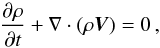 (1)
(1) (2)
(2) (3)
(3) (4)where ρ, P, V, and
B denote the density, gas pressure,
velocity, and magnetic field, respectively. The factor (4π)−1/2 is absorbed
into the definition of B, which of course is divergence free,
∇·B = 0. The gravitational potential is
given by Φ = −GM/R,
where G the
gravitational constant, M the mass of the central object, and R the spherical radius.
Finally, Γ = 5/3 is the ratio of the specific heats, and
Λ represents optically thin
radiation losses, which are presented in detail in Sect. 2.3. Even though the simulations are performed in code units, our results are
presented directly in physical units.
(4)where ρ, P, V, and
B denote the density, gas pressure,
velocity, and magnetic field, respectively. The factor (4π)−1/2 is absorbed
into the definition of B, which of course is divergence free,
∇·B = 0. The gravitational potential is
given by Φ = −GM/R,
where G the
gravitational constant, M the mass of the central object, and R the spherical radius.
Finally, Γ = 5/3 is the ratio of the specific heats, and
Λ represents optically thin
radiation losses, which are presented in detail in Sect. 2.3. Even though the simulations are performed in code units, our results are
presented directly in physical units.
2.2. Numerical models
We take several steps to set up the initial conditions of the two-component jet simulations. In summary, analytical MHD outflow solutions are employed, normalized to each other, and then properly combined. A low resolution simulation is carried out, and the final steady state saved. The output data are used to initialize our main simulations, in which we apply a velocity variability at the base, and employ optically thin radiation losses and adaptive mesh refinement (AMR), that significantly increases the effective resolution.
The ADO solution is adopted from Vlahakis et al. (2000) and describes a magneto-centrifugally accelerated disk wind that successfully crosses all three magnetosonic critical surfaces. The ASO model is taken from Sauty et al. (2002) and is a pressure-driven solution with a large lever arm capable of spinning down the protostar (see Matsakos et al. 2009, for more details on implementing the solutions).
The two-component jets are initialized with the stellar outflow replacing the inner regions of the disk wind. The normalization and combination of the solutions is based on the following numerical and physical arguments, which is an approach adopted from Matsakos et al. (2012). First, the solutions are scaled to correspond to the same central mass. Then, a matching surface is chosen at an appropriate location such that the shape of the magnetic field of the disk wind approximately matches the geometry of the ASO fieldlines. Finally, we require that the magnitude of B, which is provided by each of the analytical models on that surface, has a similar value.
The transition between the two solutions is based on the magnetic flux function
A, which
essentially labels the fieldlines of each solution (see Vlahakis et al. 2000; and Sauty et al. 2002). Initially, we create the variable A1 = AD + AS + Ac,
simply by adding the flux functions of the ADO and ASO components, with Ac a
normalization constant. We then create the variable A2 by
exponentially smoothing out the solutions around the matching surface, Amix, such that
the stellar solution dominates close to the axis and the disk wind at the outer regions;
i.e. ![Mathematical equation: \begin{equation} A_2 = \left\{1-\exp \left[-\left(\frac{A_1}{A_\mathrm{mix}}\right)^2\right]\right\} A_\mathrm{D} + \exp \left[-\left(\frac{A_1}{A_\mathrm{mix}}\right)^2 \right] A_\mathrm{S}\,. \end{equation}](/articles/aa/full_html/2014/02/aa22627-13/aa22627-13-eq26.png) (5)This new magnetic
flux function, A2, is used to initialize most of the
physical quantities U, namely ρ, P, V, A and Bφ, with the help of the
following formula:
(5)This new magnetic
flux function, A2, is used to initialize most of the
physical quantities U, namely ρ, P, V, A and Bφ, with the help of the
following formula: ![Mathematical equation: \begin{equation} U = \left\{1-\exp \left[-\left(\frac{A_2}{A_\mathrm{mix}}\right)^2\right]\right\} U_\mathrm{D} + \exp \left[-\left(\frac{A_2}{A_\mathrm{mix}}\right)^2 \right] U_\mathrm{S}\,. \end{equation}](/articles/aa/full_html/2014/02/aa22627-13/aa22627-13-eq29.png) (6)Finally, the
poloidal magnetic field is derived from the magnetic flux function; i.e.,
(6)Finally, the
poloidal magnetic field is derived from the magnetic flux function; i.e.,
 ,
hence divergent-free by definition.
,
hence divergent-free by definition.
At this stage, the two-component jet model is evolved adiabatically in time until it reaches a steady state. For efficiency, we perform the simulation on a low resolution grid, i.e., 128 zones in the radial direction and 1024 in the vertical. We point out that the level of refinement does not affect the final outcome of the simulation. On the contrary, the final configuration is a well maintained steady state, and it is obtained independently of the resolution or the mixing parameters; see Matsakos et al. (2009). The use of AMR is required for correct treatment of the cooling, as explained later, and does not affect the steady state of the adiabatic jet simulation.
This steady state is then used as initial conditions for the simulation that includes
optically thin radiation cooling, also imposing fluctuations in the flow. The variability
in the velocity is achieved by multiplying its longitudinal component with a sinusoidal
dependence in time and Gaussian in space, i.e. Vz → fSVz,
with ![Mathematical equation: \begin{equation} f_\mathrm{S}(r, t) = 1 + p\exp\left[-\left(\frac{r}{r_\mathrm{var}}\right)^2\right] \sin\left(\frac{2\pi t}{t_\mathrm{var}}\right)\,, \end{equation}](/articles/aa/full_html/2014/02/aa22627-13/aa22627-13-eq34.png) (7)where p = 20%, r is the cylindrical
radius, rvar = 50 AU, and tvar = 3.7 yr.
The variability of the velocity is chosen small enough that we can assume a constant
pre-ionization of the shocked material (Cox & Raymond 1985).
(7)where p = 20%, r is the cylindrical
radius, rvar = 50 AU, and tvar = 3.7 yr.
The variability of the velocity is chosen small enough that we can assume a constant
pre-ionization of the shocked material (Cox & Raymond 1985).
2.3. Cooling function
We take advantage of the multi-ion non-equilibrium (MINEq) cooling module developed by Teşileanu et al. (2008), which includes an ionization network and a five-level atom model for radiative transitions. Previous approaches followed the evolution in time of only the ionization of hydrogen, assuming equilibrium ionization states for the other elements of interest. In the context of strong shocks propagating and heating the plasma, as encountered in variable stellar jets, the assumption of equilibrium limited the accuracy and reliability of the simulation results.
The MINEq cooling function includes a network of a maximum of 29 ion species, selected appropriately to capture most of the radiative losses in YSO jets up to temperatures of 200 000 K. These ion species represent the first five ionization states (from I to V) of C, N, O, Ne, and S, as well as H i, H ii, He i, and He ii. In more recent versions, the cooling function implementation allows the user to select the number of ionization states required for each simulation. Depending on shock strength, some of the upper-lying ionization states may be disabled. In the present work, the first three ionization states were used, a choice that is adequate for the physical conditions developing in the areas of interest.
For each ion, one additional equation must be solved: 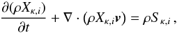 (8)coupled to the original
system of MHD equations. In this equation, the first index (κ) describes the element,
while the second index (i) corresponds to the ionization state. Specifically,
Xκ,i ≡ Nκ,i/Nκ
is the ion number fraction, Nκ,i the number
density of the i-th ion of element κ, and Nκ the element number
density. The source term Sκ,i accounts for the
effect of the ionization and recombination processes.
(8)coupled to the original
system of MHD equations. In this equation, the first index (κ) describes the element,
while the second index (i) corresponds to the ionization state. Specifically,
Xκ,i ≡ Nκ,i/Nκ
is the ion number fraction, Nκ,i the number
density of the i-th ion of element κ, and Nκ the element number
density. The source term Sκ,i accounts for the
effect of the ionization and recombination processes.
For each ion, the collisionally excited line radiation is computed, and the total line emission from these species enters in the source term Λ of Eq. (3). This provides an adequate approximation of radiative cooling for the conditions encountered in YSO jets. Depending on the conditions, more ion species may be included.
Cooling introduces an additional timescale in MHD numerical simulations, together with the dynamical one. In regions where sudden compressions/heating of the gas occur, the timescale for cooling and ionization of the gas becomes much smaller and thus dominates the simulation timestep. Consequently, a larger number of integration steps are needed, and the total duration of the simulations increases considerably.
Finally, another aspect to consider is the numerical resolution. This is required for a sufficiently accurate and reliable physical description of the processes occurring in the post-shock zone behind a shock front, especially concerning the ionization state of the plasma. As discussed in previous work, a resolution higher than 1012 cm (~0.07AU) per integration cell is needed to adequately resolve the physical parameters after the shock front (Mignone et al. 2009). Therefore, AMR is necessary in order to treat correctly the dynamics/cooling while retaining high efficiency for the simulation.
2.4. Numerical setup
We use PLUTO, a numerical code for computational astrophysics1, to carry out the MHD simulations (Mignone et al. 2007). We choose cylindrical coordinates (r,z) in 2.5D, assuming axisymmetry to suppress the third dimension. Integration is performed with the HLL solver with second order accuracy in both space and time, whereas the condition ∇·B = 0 is ensured with hyperbolic divergence cleaning. Since the jet kinematics involve length and time scales much larger that those controlled by optically thin radiation losses (e.g. the post-shock regions), AMR is adopted (Mignone et al. 2012). The refinement strategy is based on the second derivative error norm (see Mignone et al. 2012) taken for the quantity defined by the product of the temperature with radius. Such a criterion is appropriate for resolving the shocks, as well as the region around the axis.
We performed two simulations, one using the detailed MINEq cooling function and another that only evolves the ionization of H: SNEq (Simplified Non-Equilibrium cooling). Our computational box spans [0, 80] AU in the radial direction and [100, 740] AU in the longitudinal. For the model employing SNEq, the base grid is 64 × 512 with five levels of refinement that provides an effective resolution of 16 384 zones along the axis, equivalent to one cell for each 0.04 AU. For the more computationally expensive cooling module MINEq, our base grid is 32 × 256 also with five levels of refinement, equivalent to one cell per 0.08 AU. We prescribe outflow conditions on the top and right boundaries, axisymmetry on the left, and we keep fixed all quantities to their initial values on the bottom boundary. We note that the two-component jet model is initialized everywhere inside the computational box, so we do not model the bow shock or the acceleration regions, but rather a part of the outflow in between. Ionization is initialized throughout the entire integration domain with equilibrium values resulting from the local physical conditions (temperature and density).
Finally, we comment on the location of the lower edge of the computational box. Apart from the fact that the paper focuses and attempts to address the propagation scales, the choice for the height of the bottom boundary is based on the following two reasons. Firstly, the high resolution required to properly treat the launching regions of the stellar and disk outflows combined together with distances of hundreds of AU is prohibitive from the point of view of computational time. Secondly, the source term in the energy equation close to the base of the jet is complex and not well-known. The mass loading of the field lines and, in some cases, the acceleration, requires some sort of heating that involves extra assumptions and additional parameters. Instead, we have decided to take advantage of the available analytical solutions and start the computation at a large distance where such heating terms are not present.
2.5. Post-processing and emission maps
As output the code provides the maps of all physical quantities at specified intervals of time. Further treatment of the data is required before they can be directly compared to observations.
The first post-processing routine is to calculate 2D emission maps from the simulation output. The collisionally excited emission lines of observational interest treated in the present work are the forbidden emission line doublets of N ii (6584 + 6548 Å), O i (6300 + 6363 Å), and S ii (6717 + 6727 Å). Next, the 3D integration of this axially symmetric output is performed, to account for the particular geometry encountered for each source. At this stage, a tilt angle of the simulated jet with respect to the line of sight may be applied. Then, the 3D object is projected on a surface perpendicular to the line of sight (equivalent to the “plane of sky”), and the distance to the object is taken into consideration in order to convert all data to the same units as observations. A point spread function (PSF) is also applied in the simplified form of a Gaussian function with a user-defined width, in order to simulate the effect of the observing instrument2.
3. Results
3.1. Dynamics
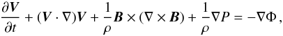
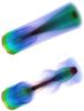 |
Fig. 1 3D representation of the density distribution of the initial conditions (top) and at a later time during evolution (bottom). Blue/red corresponds to low/high density, the thin blue lines denote the magnetic field and the thick red lines the flow. |
The initial conditions correspond to a steady-state, magnetized self-collimated jet, a configuration that is reached after the combination and adiabatic evolution of the two wind components, see top panel of Fig. 1. Its inner part represents a hot stellar outflow that is collimated by the hoop stress provided by the magnetic field of the surrounding disk wind. The longitudinal velocity decreases with radius, i.e. the flow consists of a fast jet close to the axis and a slow wind at the outer radii. During the first steps of the simulation, the cooling function lowers the temperature of the plasma, especially in the inner hot regions. Owing to the pressure drop, the collimating forces squeeze the jet, and in turn the jet radius is decreased (see bottom panel of Fig. 1 and Sect. 3.5 for a discussion). Moreover, the variability applied on the bottom boundary produces shocks that propagate along the axis and lead to the formation of a knot-structured jet. These internal shocks locally heat the gas, and in turn the post-shock regions are susceptible to larger energy losses and strong emission.
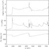 |
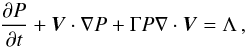
Fig. 2 Logarithmic number density (top), temperature (middle), and velocity (bottom) profiles along the axis, for the model adopting SNEq. The jet is moving from left to right and the displayed moment corresponds to t = 12 yr. |
 |
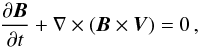
Fig. 3 Logarithmic density (top), temperature (middle), and velocity (bottom) profiles along the axis, for the model adopting MINEq. The instance corresponds to t = 12 yr. |
Figure 2 shows the average values of the number density, temperature, and velocity of the outflow around the axis (for r ≤ 0.5 AU), for the simulation performed with the SNEq module. Figure 3 displays the same quantities for the model that adopts the MINEq cooling function. The number density ranges from 104 to 105 cm-3, with higher local values at overdensities produced by the variability of the flow. A strong shock can be observed approximately at 450 AU, in accordance with the negative slope of the velocity profile. The jet temperatute is on the order of 10 000 K, but may exceed 20 000 K at the post-shock regions. The jet velocity is on average 380 km s-1, whereas the speed of the shocks relative to the bulk flow is ~100 km s-1. In general, both models correctly capture the typical values of observed YSO jets.
Even though the two simulations incorporate different cooling functions, the dynamics between the two simulations are roughly similar. This suggests that the simpler SNEq module is a good approximation for treating the energy losses during the temporal evolution. For this reason, this module is employed in a future work that studies the full 3D jet structure (Matsakos et al., in prep.). However, the aim of the present paper is to calculate line emissions, therefore in the following we focus on the simulation that adopts the MINEq cooling function.
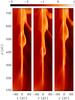 |
Fig. 4 Logarithmic maps of the density in normalized units of 104 cm-3 (left axis of each panel), and the temperature in 104 K (right axis of each panel), for the model employing the MINEq cooling. From left to right, three moments of the temporal evolution are shown, i.e., 16.8, 19.2, and 21.6 years. The jet is propagating upward, and specifically, the high density region located between 200 and 300 AU in the left panel, is found between 400 and 500 AU in the middle, and between 600 and 700 AU in the right panel. |
Figure 4 shows the 2D logarithmic distribution of the density and temperature at three evolutionary moments separated by 2.4 years. The higher density jet material defines the positions of the propagating knots. For instance, a knot that can be seen at ~250 AU in the left panel is located at ~450 AU in the central panel, and at ~650 AU in the right one. The surface close to the axis that separates the inner hot outflow from the outer cooler gas is a weak oblique shock. It forms due to the recollimation of the flow and causally disconnects the jet from its launching region since no information can propagate backwards (Matsakos et al. 2008; 2009).
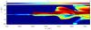 |
Fig. 5 Comparison of the logarithmic temperature distribution and jet radius for an adiabatic evolution (top) and with the MINEq cooling module (bottom). The snapshot corresponds to t = 21.6. |
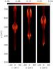 |
Fig. 6 Maps of the total ionization fraction of the jet material for the three moments in the evolution shown in Fig. 4. |
To estimate the effects of the energy losses on the dynamics of the jet, we plot in Fig. 5 the temperature distribution of an adiabatic evolution (top), together with that of the simulation adopting MINEq (bottom). Optically thin radiation reduces the pressure of the inner hot flow, so the radius of the emitting jet is found by a factor of 2 to be smaller than the adiabatic one because of the unbalanced collimating forces. On the other hand, the predicted temperature of the adiabatic model can be an order of magnitude higher, which in turn may lead to overestimating the emission.
Since the final configuration of the adiabatic simulation shows a different morphology than the one with the imposed cooling, we should examine the bottom boundary conditions for consistency. Namely, we should check whether the quantities imposed at the lower edge of the MINEq simulation, which are given by the adiabatic model, affect or enforce the evolution of the system. However, the effects of the optically thin radiation cooling are significant mainly where the outflow is hot, i.e. close to the axis (Fig. 5). In turn, both at the base of the computational box and at outer radii, the adiabatic evolution is very similar to the one with cooling. Therefore, we argue that the bottom boundary conditions are consistent with the MINEq simulation.
3.2. Ionization
In the analytical models employed here, no pre-existing condition of ionization of the jet material was set. Ionization is self-consistently computed during the evolution, snapshots of which are shown in Fig. 6. The flow is locally ionized when the temperature rises, and as a result, the jet ionization is very low close to the origin and gets higher within the knots (~34%). The degree of pre-ionization may affect the line emission, as discussed in Teşileanu et al. (2012).
3.3. Emission maps
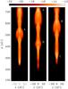 |
Fig. 7 Logarithmic maps of the surface brightness of the forbidden doublet [S ii], convolved with the PSF, for the three moments shown in Fig. 4. The image is in units of erg cm-2 arcsec-2 s-1 and has been projected with a declination angle of 80° with respect to the line of sight. The knots are labeled with letters. |
Post-processing was applied to the simulation employing the sophisticated cooling function MINEq. In Fig. 7, surface brightness maps of [S ii] are shown for the corresponding three outputs of Fig. 4, after having also applied a declination angle of 80°. The outflow appears as a prominent well-collimated jet with a small opening angle. In fact, the overall emission seems to originate in the region enclosed by the weak oblique shock discussed in Sect. 3.1. For our model, this suggests that the mechanism responsible for heating the bulk of the flow at the temperatures required for an observable emission is the effect of recollimation, which compresses the flow around the axis. The presence of the less dense and slower surrounding wind cannot be seen in this emission line. Nevertheless, it fills up the rest of the computational domain and is considered to emanate from the outer disk radii, contributing to the mass and angular momentum loss rates.
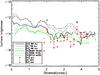 |
Fig. 8 Logarithmic surface brightness profiles of the forbidden doublets along the axis [S ii], [N ii], and [O i], for two observed YSO jets (RW Aurigae and HH 30) and the MINEq simulation. The image is in units of erg cm-2 arcsec-2 s-1 and corresponds to t = 21.6 yr. |
Moreover, emission knots are observed along the jet axis, which correspond to high-density and temperature regions produced by the propagating shocks. The knots have an enhanced surface brightness that can be ten times higher than the bulk flow (see Fig. 8). The introduced variability has been intentionally chosen to be a few years, producing knot structures every few hundred AU. This is the typical length scale observed in YSO jets, such as in the systems HH 1&2, HH 34, and HH 47, for which high angular resolution astronomical data are available (e.g., Hartigan et al. 2011).
Furthermore, Fig. 8 directly compares the line emissions given by the simulation with those of two observed jets, RW Aur and HH 30. The plot suggests good agreement in the intensities at large distances from the origin of the outflow. In fact, the emission coming from the bulk flow of this model is closer to observations than the earlier work of Teşileanu et al. (2012). The improvement is attributed to the heating provided by the recollimation of the flow. Moreover, a pre-existing ionization would provide higher emissivity in the regions between the knots, bringing the model closer to observations.
The discrepancy close to the source might be evidence that there are additional mechanisms in the first part of the jet propagation, such as a pre-existing heating and ionization of the gas that can increase emissivity (e.g., Teşileanu et al. 2012). On the other hand, the flow has to propagate for a certain distance before the induced sinusoidal time dependence can form shocks. In addition, the jet is initially expanding before it recollimates and heats the gas. Low emission close to the central object is also found observationally, for instance, in the jets HH 34, HH 211, and HH 212 (Correira et al. 2009). However, the length of the low emissivity region of those objects is larger at least by an order of magnitude than here, and also the corresponding mechanisms and/or the parameters used in the present simulation may be different.
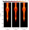 |
Fig. 9 Logarithmic maps of the surface brightness, processed as described in Fig. 7, for the three forbidden doublets of [O i], [N ii], and [S ii] (from left to right), in units of erg cm-2 arcsec-2 s-1. The snapshot corresponds to t = 21.6 yr. |
Finally, Fig. 9 displays the surface brightness maps for the three forbidden doublets of [O i], [N ii], and [S ii] for the last evolutionary moment displayed in Fig. 4. All three panels highlight the same structure. The two knots, located slightly above ~300 AU and ~600 AU, emit more strongly than the rest of the flow and can be clearly seen in all three emission lines. We have not simulated the bow shock where the outflow interacts with the interstellar medium, since our initial conditions did not include it.
3.4. PV diagram
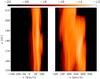 |
Fig. 10 Position–velocity diagrams for a declination angle with the line of sight of 80° (left) and 45° (right), for the forbidden doublet of [S ii]. Units in erg cm-2 arcsec-2 s-1. |
Figure 10 displays examples of the position–velocity (PV) contours, a diagram that is widely used for representing the observational data of YSO jets. It shows the distribution of the brightness with respect to the position along the spectrometer slit and the velocity along the line of sight. We chose two declination angles for the reconstructed 3D distribution and an arbitrary slit width of 20 AU positioned along the central jet axis. In the case of a jet almost perpendicular to the line of sight (80°, left panel), the projection of the longitudinal speed is small, so that a value of ~60 km s-1 is recovered at all heights, with deviations of a few tenths of km s-1. However, when the angle between the line of sight and the outflow axis is smaller (45°, right panel) the projected component is larger, around ~250 km s-1. The distribution of velocities is also wider, ~50 km s-1, since the flow fluctuations can now be observed. In addition, the figure brings out those parts of the flow that propagate faster and the speed distribution can thus be inferred and associated with the observed knot structures.
For the latter case of a lower declination angle with respect to the line of sight, the surface brightness maps in the emission lines of interest are similar to Fig. 9, apart from the distance between the knots, which seems shorter due to projection effects.
3.5. Jet radius
We proceed to calculate the jet radius from Fig. 9. We follow a simple approach based on the full width half maximum method. The maximum at each height of the emission map is calculated, and then the radius where the distribution takes half that value is determined. Since the plot is logarithmic, the background emission is required in order to correctly compute the height of the distribution over the radius. We considered this parameter to be 10-26 erg cm-2 arcsec-2 s-1, but we note that values that are different by a few orders of magnitude provide almost the same result.
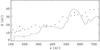 |
Fig. 11 Jet radius (solid line), R, as computed from the average of the doublets O i, N ii, and S ii for t = 21.6. Diamonds denote observations of RW Aur, stars of HH 30, and triangles of HL Tau. |
Figure 11 plots the jet radius, R, as computed from the average of the doublets O i, N ii, and S ii. Data points of the jets RW Aur, HH 30, and HL are also shown for comparison. The plot suggests a jet width of 40 to 60 AU, in good agreement with observations (Ray et al. 2007, and references therein). The variations in R along the axis is due to the applied speed variability. However, this does not seem to disrupt the average width, even though it introduces local deviations. Apart from the jet radius, the opening angle is also comparable and is a few degrees.
Stute et al. (2010) find similar jet radii for their truncated disk-wind solution. The radii for the untruncated cases were much larger than in the present study, mostly because of the absence of the cooling term in the energy equation, which resulted in much higher temperatures.
4. Summary and conclusions
In this paper, we started from a combination of two analytical outflow solutions, a stellar jet and a disk wind; we simulated the two-component jet; and we then generated synthetic emission maps. We carried out 2.5D axisymmetric numerical simulations that adopt a sophisticated cooling function that follows the ionization and optically thin radiation losses of several ions. We also applied a velocity variability at the base of the outflow in order to produce shocks and knots along the axis.
Our conclusions can be summarized as follows:
-
1.
The dynamical evolution of the two-component jet model is similar whether a simplified or a detailed cooling function is adopted. However, the adiabatic case leads to the overestimation of the jet radius by a factor of 2 and the temperature by an order of magnitude.
-
2.
The density, temperature, and velocity along the axis are within the typical value range of observed astronomical sources.
-
3.
Apart from the above physical parameters, the jet radius, as well as the opening angle, is also found to be close to typical YSO jets.
-
4.
The dense and hot inner part of the jet emits strongly, with the synthetic emission maps showing a well-collimated outflow that closely resembles real observations. The emission knots propagate along the axis and demonstrate enhanced emission because they are dense post-shock regions.
-
5.
The predicted emission lines match the observations of YSO jets at high altitudes, but they have lower values close to the source. We speculate that by taking heating and pre-ionization into account at the base of the flow might reduce this discrepancy.
Our results are very encouraging and prompt for further investigation. By closing the gap between analytical solutions, numerical simulations, and observations, valuable feedback is provided that will help improve the outflow models further, and help understand the jet phenomenology more deeply. The simulations reported here are axisymmetric and may be expanded to allow nonaxisymmetric perturbations. However, the recent 3D simulations of disk-winds crossing the FMSS have shown that the analytical MHD solutions behave well even when the basic assumption of axisymmetry is relaxed (Stute et al. 2014).
In a future work, we plan to model specific YSO jets in an attempt to recover their properties and understand their dynamics. Further work will also focus on introducing pre-existing ionization of the jet material, which will probably improve the agreement of the simulation results with observations. From the point of view of synthetic observations, the present results seem to be complemented by the ones previously published in Teşileanu et al. (2012) for the first part of jet propagation (the first 2 arcsec).
Freely available at http://plutocode.ph.unito.it
All post-processing routines are included in user-friendly templates in the current distribution of the PLUTO code.
Acknowledgments
We are grateful to the anonymous referee whose constructive report resulted in improving and clarifying several parts of the paper. This research was supported by a Marie Curie European Reintegration Grant within the 7th European Community Framework Program, (“TJ-CompTON”, PERG05-GA-2009-249164), and also partly by the ANR STARSHOCK project ANR-08-BLAN-0263-07-2009/2013. The numerical simulations were performed on the cluster at the Laboratory of Computational Astrophysics at the Faculty of Physics, University of Bucharest. The contribution of OT is based on the research performed during the project financed by contract CNCSIS-RP no. 4/1.07.2009 (2009-2011) in the Romanian PNII framework.
References
- Anderson, J., Li, Z.-Y., Krasnopolsky, R., & Blandford, R. 2005, ApJ, 630, 945 [NASA ADS] [CrossRef] [Google Scholar]
- Blandford, R. D., & Payne, D. G. 1982, MNRAS, 199, 883 [NASA ADS] [CrossRef] [Google Scholar]
- Cabrit, S., Edwards, S., Strom, S. E., & Strom, K. M. 1990, ApJ, 354, 687 [NASA ADS] [CrossRef] [Google Scholar]
- Cabrit, S., Ferreira, J., & Raga, A. C. 1999, A&A, 343, L61 [Google Scholar]
- Casse, F., & Keppens, R. 2002, ApJ, 581, 988 [NASA ADS] [CrossRef] [Google Scholar]
- Casse, F., & Keppens, R. 2004, ApJ, 601, 90 [NASA ADS] [CrossRef] [Google Scholar]
- Čemeljić, M., Gracia, J., Vlahakis, N., & Tsinganos, K. 2008, MNRAS, 389, 1022 [NASA ADS] [CrossRef] [Google Scholar]
- Correia, S., Zinnecker, H., Ridgway, S. T., & McCaughrean, M. J. 2009, A&A, 505, 673 [NASA ADS] [CrossRef] [EDP Sciences] [Google Scholar]
- Cox, D., & Raymond, J. 1985, ApJ, 298, 651 [NASA ADS] [CrossRef] [Google Scholar]
- Dougados, C., Cabrit, S., Lavalley, C., & Ménard, F. 2000, A&A, 357, L61 [NASA ADS] [Google Scholar]
- Edwards, S., Fischer, W., Hillenbrand, L., & Kwan, J. 2006, ApJ, 646, 319 [NASA ADS] [CrossRef] [Google Scholar]
- Eislöffel, J., & Mundt, R. 1992, A&A, 263, 292 [NASA ADS] [Google Scholar]
- Eislöffel, J., Mundt, R., & Böhm, K.-H. 1994, AJ, 108, 1042 [NASA ADS] [CrossRef] [Google Scholar]
- Fendt, C. 2006, ApJ, 651, 272 [NASA ADS] [CrossRef] [Google Scholar]
- Fendt, C. 2009, ApJ, 692, 346 [NASA ADS] [CrossRef] [Google Scholar]
- Fendt, C., & Sheikhnezami, S. 2013, ApJ, 774, 12 [NASA ADS] [CrossRef] [Google Scholar]
- Ferreira, J., Dougados, C., & Cabrit, S. 2006, A&A, 453, 785 [NASA ADS] [CrossRef] [EDP Sciences] [Google Scholar]
- Gracia, J., Vlahakis, N., & Tsinganos, K. 2006, MNRAS, 367, 201 [NASA ADS] [CrossRef] [Google Scholar]
- Hartigan, P., Edwards, S., & Ghandour, L. 1995, ApJ, 452, 736 [NASA ADS] [CrossRef] [Google Scholar]
- Hartigan, P., Edwards, S., & Pierson, R. 2004, ApJ, 609, 261 [NASA ADS] [CrossRef] [Google Scholar]
- Hartigan, P., Frank, A., Foster, J. M., et al. 2011, ApJ, 736, 29 [Google Scholar]
- Krasnopolsky, R., Li, Z.-Y., & Blandford, R. 1999, ApJ, 526, 631 [NASA ADS] [CrossRef] [Google Scholar]
- Kwan, J., Edwards, S., & Fischer, W. 2007, ApJ, 657, 897 [NASA ADS] [CrossRef] [Google Scholar]
- Lynden-Bell, D., & Pringle, J. E. 1974, MNRAS, 168, 603 [NASA ADS] [CrossRef] [Google Scholar]
- Massaglia, S., Mignone, A., & Bodo, G. 2005, A&A, 442, 549 [NASA ADS] [CrossRef] [EDP Sciences] [Google Scholar]
- Matsakos, T., Tsinganos, K., Vlahakis, N., et al. 2008, A&A, 477, 521 [NASA ADS] [CrossRef] [EDP Sciences] [Google Scholar]
- Matsakos, T., Massaglia, S., Trussoni, E., et al. 2009, A&A, 502, 217 [NASA ADS] [CrossRef] [EDP Sciences] [Google Scholar]
- Matsakos, T., Vlahakis, N., Tsinganos, K., et al. 2012, A&A, 545, A53 [NASA ADS] [CrossRef] [EDP Sciences] [Google Scholar]
- Matt, S., & Pudritz, R. 2008, ApJ, 678, 1109 [Google Scholar]
- Matt, S., Pinzón, G., Greene, T., & Pudritz, R. 2012, ApJ, 745, 101 [NASA ADS] [CrossRef] [Google Scholar]
- Meliani, Z., Casse, F., & Sauty, C. 2006, A&A, 460, 1 [NASA ADS] [CrossRef] [EDP Sciences] [Google Scholar]
- Mignone, A., Bodo, G., Massaglia, S., et al. 2007, ApJS, 170, 228 [Google Scholar]
- Mignone, A., Teşileanu, O., & Zanni, C. 2009, ASP Conf. Ser., 406, 105 [NASA ADS] [Google Scholar]
- Mignone, A., Zanni, C., Tzeferacos, P., et al. 2012, ApJS, 198, 7 [Google Scholar]
- Ouyed, R., & Pudritz, R. 1997a, ApJ, 482, 712 [NASA ADS] [CrossRef] [Google Scholar]
- Ouyed, R., & Pudritz, R. 1997b, ApJ, 484, 794 [Google Scholar]
- Ouyed, R., & Pudritz, R. 1999, MNRAS, 309, 233 [NASA ADS] [CrossRef] [Google Scholar]
- Parker, E. N. 1958, ApJ, 128, 664 [Google Scholar]
- Pudritz, R., Rogers, C., & Ouyed, R. 2006, MNRAS, 365, 1131 [NASA ADS] [CrossRef] [Google Scholar]
- Ray, T. P., Mundt, R., Dyson, J. E., Falle, S. A. E. G., & Raga, A. C. 1996, ApJ, 468, L103 [NASA ADS] [CrossRef] [Google Scholar]
- Ray, T. P., Dougados, C., Bacciotti, F., et al. 2007, in Protostars and Planets V, eds. B. Reipurth, D. Jewitt, & K. Keil (University of Arizona Press), 231 [Google Scholar]
- Reipurth, B., & Bally, J. 2001, ARA&A, 39, 403 [NASA ADS] [CrossRef] [Google Scholar]
- Sauty, C., & Tsinganos, K. 1994, A&A, 287, 893 [NASA ADS] [Google Scholar]
- Sauty, C., Trussoni, E., & Tsinganos, K. 2002, A&A, 389, 1068 [NASA ADS] [CrossRef] [EDP Sciences] [Google Scholar]
- Sauty, C., Meliani, Z., Lima, J. J. G., et al. 2011, A&A, 533, A46 [NASA ADS] [CrossRef] [EDP Sciences] [Google Scholar]
- Sauty, C., Cayatte, V., Lima, J. J. G., Matsakos, T., & Tsinganos, K. 2012, ApJ, 759, L1 [NASA ADS] [CrossRef] [Google Scholar]
- Sheikhnezami, S., Fendt, C., Porth, O., Vaidya, B., & Ghanbari, J. 2012, ApJ, 757, 65 [NASA ADS] [CrossRef] [Google Scholar]
- Staff, J., Niebergal, B., Ouyed, R., Pudritz, R., & Cai, K. 2010, ApJ, 722, 1325 [NASA ADS] [CrossRef] [Google Scholar]
- Stute, M., Tsinganos, K., Vlahakis, N., Matsakos, T., & Gracia, J. 2008, A&A, 491, 339 [NASA ADS] [CrossRef] [EDP Sciences] [Google Scholar]
- Stute, M., Gracia, J., Tsinganos, K., & Vlahakis, N. 2010, A&A, 516, A6 [NASA ADS] [CrossRef] [EDP Sciences] [Google Scholar]
- Stute, M., Gracia, J., Vlahakis, et al. 2014, MNRAS, submitted [arXiv:1402.0002] [Google Scholar]
- Teşileanu, O., Mignone, A., & Massaglia, S. 2008, A&A, 488, 429 [NASA ADS] [CrossRef] [EDP Sciences] [Google Scholar]
- Teşileanu, O., Massaglia, S., Mignone, A., Bodo, G., & Bacciotti, F. 2009, A&A, 507, 581 [NASA ADS] [CrossRef] [EDP Sciences] [Google Scholar]
- Teşileanu, O., Mignone, A., Massaglia, S., & Bacciotti, F. 2012, ApJ, 746, 96 [NASA ADS] [CrossRef] [Google Scholar]
- Trussoni, E., Tsinganos, K., & Sauty, C. 1997, A&A, 325, 1099 [NASA ADS] [Google Scholar]
- Tsinganos, K. 2007, in Jets from Young Stars: Models and Constraints, Lecture Notes in Physics, eds. J. Ferreira, C. Dougados, & E. Whelan (Springer Verlag), 723, 117 [Google Scholar]
- Tzeferacos, P., Ferrari, A., Mignone, A., et al. 2009, MNRAS, 400, 820 [NASA ADS] [CrossRef] [Google Scholar]
- Tzeferacos, P., Ferrari, A., Mignone, A., et al. 2013, MNRAS, 428, 3151 [NASA ADS] [CrossRef] [Google Scholar]
- Vlahakis, N., & Tsinganos, K. 1998, MNRAS, 298, 777 [NASA ADS] [CrossRef] [Google Scholar]
- Vlahakis, N., Tsinganos, K., Sauty, C., & Trussoni, E. 2000, MNRAS, 318, 417 [NASA ADS] [CrossRef] [Google Scholar]
- Zanni, C., Ferrari, A., Rosner, R., Bodo, G., & Massaglia, S. 2007, A&A, 469, 811 [NASA ADS] [CrossRef] [EDP Sciences] [Google Scholar]
All Figures
|
Fig. 1 3D representation of the density distribution of the initial conditions (top) and at a later time during evolution (bottom). Blue/red corresponds to low/high density, the thin blue lines denote the magnetic field and the thick red lines the flow. |
| In the text | |
|
Fig. 2 Logarithmic number density (top), temperature (middle), and velocity (bottom) profiles along the axis, for the model adopting SNEq. The jet is moving from left to right and the displayed moment corresponds to t = 12 yr. |
| In the text | |
|
Fig. 3 Logarithmic density (top), temperature (middle), and velocity (bottom) profiles along the axis, for the model adopting MINEq. The instance corresponds to t = 12 yr. |
| In the text | |
|
Fig. 4 Logarithmic maps of the density in normalized units of 104 cm-3 (left axis of each panel), and the temperature in 104 K (right axis of each panel), for the model employing the MINEq cooling. From left to right, three moments of the temporal evolution are shown, i.e., 16.8, 19.2, and 21.6 years. The jet is propagating upward, and specifically, the high density region located between 200 and 300 AU in the left panel, is found between 400 and 500 AU in the middle, and between 600 and 700 AU in the right panel. |
| In the text | |
|
Fig. 5 Comparison of the logarithmic temperature distribution and jet radius for an adiabatic evolution (top) and with the MINEq cooling module (bottom). The snapshot corresponds to t = 21.6. |
| In the text | |
|
Fig. 6 Maps of the total ionization fraction of the jet material for the three moments in the evolution shown in Fig. 4. |
| In the text | |
|
Fig. 7 Logarithmic maps of the surface brightness of the forbidden doublet [S ii], convolved with the PSF, for the three moments shown in Fig. 4. The image is in units of erg cm-2 arcsec-2 s-1 and has been projected with a declination angle of 80° with respect to the line of sight. The knots are labeled with letters. |
| In the text | |
|
Fig. 8 Logarithmic surface brightness profiles of the forbidden doublets along the axis [S ii], [N ii], and [O i], for two observed YSO jets (RW Aurigae and HH 30) and the MINEq simulation. The image is in units of erg cm-2 arcsec-2 s-1 and corresponds to t = 21.6 yr. |
| In the text | |
|
Fig. 9 Logarithmic maps of the surface brightness, processed as described in Fig. 7, for the three forbidden doublets of [O i], [N ii], and [S ii] (from left to right), in units of erg cm-2 arcsec-2 s-1. The snapshot corresponds to t = 21.6 yr. |
| In the text | |
|
Fig. 10 Position–velocity diagrams for a declination angle with the line of sight of 80° (left) and 45° (right), for the forbidden doublet of [S ii]. Units in erg cm-2 arcsec-2 s-1. |
| In the text | |
|
Fig. 11 Jet radius (solid line), R, as computed from the average of the doublets O i, N ii, and S ii for t = 21.6. Diamonds denote observations of RW Aur, stars of HH 30, and triangles of HL Tau. |
| In the text | |
Current usage metrics show cumulative count of Article Views (full-text article views including HTML views, PDF and ePub downloads, according to the available data) and Abstracts Views on Vision4Press platform.
Data correspond to usage on the plateform after 2015. The current usage metrics is available 48-96 hours after online publication and is updated daily on week days.
Initial download of the metrics may take a while.