| Issue |
A&A
Volume 562, February 2014
|
|
|---|---|---|
| Article Number | A42 | |
| Number of page(s) | 10 | |
| Section | Stellar structure and evolution | |
| DOI | https://doi.org/10.1051/0004-6361/201321383 | |
| Published online | 04 February 2014 | |
Phase-resolved X-ray spectroscopy and spectral energy distribution of the X-ray soft polar RS Caeli⋆
1 Leibniz-Institut für Astrophysik Potsdam (AIP), An der Sternwarte 16, 14482 Potsdam, Germany
e-mail: This email address is being protected from spambots. You need JavaScript enabled to view it.
2 Institut für Astrophysik, Georg-August-Universität Göttingen, Friedrich-Hund-Platz 1, 37077 Göttingen, Germany
3 Department of Physics and Astronomy, Stony Brook University, Stony Brook, NY 11794-3800, USA
4 Max-Planck-Institut für extraterrestrische Physik, PO Box 1312, 85741 Garching, Germany
Received: 28 February 2013
Accepted: 6 December 2013
Abstract
Context. RS Cae is the third target in our series of XMM-Newton observations of soft X-ray-dominated polars.
Aims. Our observational campaign aims to better understand and describe the multiwavelength data, the physical properties of the system components, and the short- and long-term behavior of the component fluxes in RS Cae.
Methods. We employ stellar atmosphere, stratified accretion-column, and widely used X-ray spectral models. We fit the XMM-Newton spectra, model the multiband light curves, and opt for a mostly consistent description of the spectral energy distribution.
Results. Our XMM-Newton data of RS Cae are clearly dominated by soft X-ray emission. The X-ray light curves are shaped by emission from the main accretion region, which is visible over the whole orbital cycle, interrupted only by a stream eclipse. The optical light curves are formed by cyclotron and stream emission. The XMM-Newton X-ray spectra comprise a black-body-like and a plasma component at mean temperatures of 36 eV and 7 keV. The spectral fits give evidence of a partially absorbing and a reflection component. Multitemperature models, covering a broader temperature range in the X-ray emitting accretion regions, reproduce the spectra appropriately well. Including archival data, we describe the spectral energy distribution with a combination of models based on a consistent set of parameters and derive a lower limit estimate of the distance d ≳ 750 pc.
Conclusions. The high bolometric soft-to-hard flux ratios and short-term variability of the (X-ray) light curves are characteristic of inhomogeneous accretion. RS Cae clearly belongs in the group of polars that show a very strong soft X-ray flux compared to their hard X-ray flux. The different black-body fluxes and similar hard X-ray and optical fluxes during the XMM-Newton and ROSAT observations show that soft and hard X-ray emission are not directly correlated.
Key words: novae, cataclysmic variables / stars: fundamental parameters / stars: individual: RS Caeli / X-rays: binaries / accretion, accretion disks
Based on observations obtained with XMM-Newton, an ESA science mission with instruments and contributions directly funded by ESA Member States and NASA.
© ESO, 2014
1. Introduction
Thirty X-ray soft polars with negative hardness ratios1 HR1 have been identified in the ROSAT all-sky survey (RASS) source catalog (Voges et al. 1999) by Thomas et al. (1998), Beuermann et al. (1999), and Schwope et al. (2002). They are potential members of the subgroup of AM Her-type systems that show a “soft X-ray excess”, i.e., a significant dominance of soft X-ray (E ≲ 0.5 keV) over hard X-ray (E ≳ 0.5 keV) luminosity, reviewed for example by Ramsay et al. (1994), Beuermann & Schwope (1994), and Beuermann & Burwitz (1995). Ramsay & Cropper (2004) demonstrated the dependence of the soft-to-hard luminosity ratios on calibration, geometrical effects, and spectral models. Using accretion-column models (Cropper et al. 1999) for recalibrated ROSAT and XMM-Newton spectra, they came to the conclusion that fewer systems show a distinct soft X-ray excess than originally estimated from the ROSAT detections.
RS Caeli was among the softest X-ray sources at the epoch of the RASS observations, with a hardness ratio of HR1 = −1.00(1). It was detected as an extreme ultraviolet source in the ROSAT/WFC and in the EUVE surveys (Pounds et al. 1993; Bowyer et al. 1994). Burwitz et al. (1996) published the first pointed X-ray and additional optical observations of RS Cae. They derived an optical apparent magnitude of mV ~ 19m, an X-ray flux on the order of 10-11 erg cm-2 s-1 in the ROSAT energy band, a distance to the binary of at least 440 pc, and a magnetic field strength B = 36(1) MG for the white-dwarf primary. The pronounced phase-dependent cyclotron harmonics in the optical spectra could be modeled for two possible accretion geometries: a binary inclination of i ~ 60° and a colatitude of the accretion region of β ~ 25°, or i ~ 25° and β ~ 60°. In the first case, stream absorption dips should be seen in the X-ray light curves. They found two candidate orbital periods of  or
or  , giving preference to the longer one. The optical spectra showed no clear signature of the M-star secondary.
By exploiting new XMM-Newton data of polars that had not been observed in X-rays since ROSAT, we are studying their system properties and the energy balance, in particular during high states (AI Tri, Traulsen et al. 2010, RS Cae, this work) and intermediate high states of accretion (AI Tri, QS Tel, Traulsen et al. 2010, 2011). In this paper, we present our third pointed XMM-Newton observation of a soft X-ray selected polar. Section 2 introduces the X-ray and optical data of RS Cae on which our analysis is based. In Sect. 3, we describe the multiwavelength light curves and confirm the orbital binary period of  . Section 4 is dedicated to the X-ray spectra, the spectral models, and the derived parameters. The whole spectral energy distribution (SED), an approach to a consistent modeling of spectra and light curves, and the implications on the system geometry are presented in Sect. 5. We close the paper with a discussion of the component fluxes and the energy budget of RS Cae in Sect. 6.
2. Observations and data reduction
RS Cae was scheduled for a 50 ks observation with XMM-Newton on March 12/13, 2009 (observation ID 0554740801). Owing to background radiation, the EPIC/pn and MOS exposures had to be stopped after 35 ks and 39 ks, respectively. All three EPIC detectors were operated in full frame mode with the thin filter. Using standard sas v9.0 tasks, we extracted light curves and spectra from circular source regions on the EPIC chips with a radius of 27.5 arcsec for EPIC/pn and of 22.5 arcsec for EPIC/MOS. We used large circular background regions with radii between 75 and 100 arcsec on the same chip as the source for the background correction. Spectra were taken from the first 28 ks of the exposure, excluding the high-background intervals. During our pointing, the source reached net peak count rates2 of 1.64 ± 0.04 cts s-1 for EPIC/pn, 0.16 ± 0.01 cts s-1 for MOS1, and 0.24 ± 0.02 cts s-1 for MOS2, which is in the range that can be expected from the ROSAT All-Sky Survey results (Voges et al. 1999) for a high-state observation. The net source count rate measured with RGS was consistent with zero.
With the optical monitor OM, we performed fast-mode photometry consecutively in the 3000−3900 Å band using the U filter (mean net count rate3 1.06 ± 0.02 cts s-1), in the 2450−3200 Å band using the UVW1 (0.53 ± 0.02 cts s-1), and in the 2050−2450 Å band using the UVM2 filter (0.13 ± 0.01 cts s-1). The exposure times of 8.2 ks per light-curve segment corresponded to about 1.3 orbital cycles. We extracted fast-mode light curves using the sas v10.0 version of the source detection algorithm and the task omfchain and took the background information from the imaging data. The UVM2 data were mostly affected by the increased background. For the rest of the visit, the optical monitor was operated with the grism1 filter (2000−3500 Å). This part of the observation fell completely in the time interval of high background radiation. Three of the fourteen scheduled 800 s exposures were taken, but are unusable due to a low signal-to-noise ratio.
Barycentric timings and 1σ errors of the dip centers in the XMM-Newton light curves of RS Cae.
To trigger the XMM-Newton observation, we repeatedly obtained optical photometry of RS Cae between December 2008 and March 2009 at the CTIO 1.3 m telescope/ANDICAM, operated by the SMARTS consortium. Two of the B-band light curves cover more than one orbital period: one taken on September 22, 2008 during a low state of accretion and one taken simultaneously to the last part of the XMM-Newton observations. Each of them comprises 32 data points with integration times of 180 s and a time resolution of 226−227 s. Photometry was done relative to stars in the field as described in Gerke et al. (2006).
We converted the ground-based data from UTC to terrestrial time TT, consistently with the satellite data, and corrected all times used in this paper to the barycenter of the solar system using the JPL ephemeris (Standish 1998).
3. Multiband light curves and photometric period
Figure 1 gives a synopsis of the X-ray, ultraviolet, and optical light curves of RS Cae. The corresponding X-ray light-curve profiles are shown in Fig. 2. Our phase convention refers to the centers of the pronounced X-ray dips and is derived in Sect. 3.1.
The XMM-Newton X-ray light curves (Figs. 1a, b, and 2) show clear periodicity that could not be detected in the 1992 ROSAT/PSPC light-curve segments presented by Burwitz et al. (1996). With EPIC/pn, about 21 400 source counts were collected in the soft X-ray band at energies below 0.5 keV and about 760 in the hard X-ray band at energies above 0.5 keV. Correspondingly, the hardness ratios HRXMM = (HX − SX)/(HX + SX) between hard (HX,0.5−10.0 keV) and soft (SX,0.1−0.5 keV) counts are remarkably low (Fig. 1c). During a sharp recurring light-curve dip, the EPIC count rates almost drop to zero for 0.07 in phase, and the hardness ratios increase. This dip is visible in all X-ray bands and coincides with ultraviolet and optical light-curve minima. The optical and ultraviolet light curves (Figs. 1d and e) are double-humped with semi-amplitudes between 0.5 and 0.7 mag, showing similar shapes during high and low states of accretion (Fig. 3). A minimum with a depth of about Δmag ~ 0.8 occurs at the time of maximum X-ray flux. They resemble the double-humped white light curves of Burwitz et al. (1996), taken in October 1992 and September 1993.
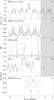 |
Fig. 1 September 2009 light curves of RS Cae in time bins of 100 s, folded on the orbital period with the center of the X-ray dips defining phase zero (Eq. (1)). The grey area marks the interval of high background activity during the XMM-Newton pointing. a)–b) Energy-resolved EPIC/pn light curves. c) Corresponding hardness ratios HRXMM = (HX − SX)/(HX + SX). d) Optical and ultraviolet light curves measured subsequently with three filters at the optical monitor. e) Optical B-band light curve with a time resolution of about 227 s, plotted twice and shifted by − 3 and − 2 orbital cycles, respectively. |
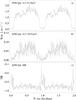 |
Fig. 2 Phase-averaged X-ray light curves, excluding the high-background interval, in time bins of 60 s and with the same phase convention and energy ranges as in Fig. 1. a–b) Energy-resolved EPIC/pn light curves. c) Corresponding hardness ratios. |
3.1. X-ray ephemeris
Burwitz et al. (1996) determined a spectroscopic ephemeris for the system and referred to the times of minimum spectral flux as phase zero. Using the recurrent X-ray dips to constrain the binary period, we can confirm their preferred period of Porb = 102 min = 0.071 d independently by Lomb-Scargle analysis, epoch folding, and a least-squares method to compute the maximum of 1/Σ(O − C)2 (observed minus calculated dip times). Observed dip times and 1σ errors are derived by Gaussian fits to Δϕ ~ 0.2 segments in the 10 s-binned EPIC/pn light curve (Table 1). The photometric ephemeris is calculated by an error-weighted fit to the observed dip times using 1ms-spaced trial periods within a ± 3σ search interval around the longer period of Burwitz et al. (1996).  (1)defines phase zero throughout the paper. The uncertainties of the last digit, given in parentheses, are 1σ errors of the O − C method.
3.2. The nature of the soft X-ray dip
Light-curve dips may occur due to an eclipse by the secondary star, a self-eclipse of the accretion region, or stream absorption. A self-eclipse is unlikely for a geometry with i + β < 90°, which is expected for RS Cae. The dips in the optical and UV light curves around phase zero resemble a (partial) eclipse feature. In Sect. 5.3, however, we show that the modulation of these light curves is mostly due to cyclotron emission and that their minima can be explained without assuming an eclipse by the secondary. We conclude that the sharp dip in the X-ray light curves is caused by absorption in the accretion stream when it crosses our line of sight towards the accretion region: (i) the hardness ratios increase rapidly at dip times, where photons at lower X-ray energies are more strongly absorbed than those at higher energies; (ii) the depth of the minima varies slightly from cycle to cycle; (iii) accretion-stream and absorption models for RS Cae following Silva et al. (2011) reproduce the X-ray dip. The X-ray dip appears to be broader toward higher energies (Fig. 4). The energy dependence may indicate that more extended, cooler parts of the accretion region are still visible, while the harder emission region is absorbed by the dense core of the stream.
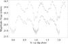 |
Fig. 3 SMARTS B-band light curves of RS Cae obtained at 2008/09/22 during a low state and at 2009/03/12 during a high state of accretion, each folded on a period of |

4. X-ray spectroscopy
From the first 28 ks of our XMM-Newton exposure, we extract EPIC/pn, MOS1, and MOS2 spectra as described in Sect. 2, excluding the phases around the X-ray light curve dips ϕX−ray ~ 0.9−1.1, and fit them simultaneously to derive general system parameters such as temperatures in the accretion region, plasma abundances, and the amount of intrinsic absorption. The EPIC spectra show the typical components of ROSAT-discovered polars: (i) the black-body like, X-ray soft emission, which can be attributed to the accretion-heated surface of the white dwarf (Sect. 4.1); and (ii) the bremsstrahlung-like, X-ray hard component, which can be attributed to the hot accretion column above the white-dwarf surface (Sect. 4.2). Since a very strong soft X-ray component was seen in the ROSAT/PSPC spectra and almost 97% of the EPIC/pn source counts are measured at energies below 0.5 keV, we are investigating in particular the soft and hard X-ray fluxes that we derive from the different spectral model approaches and discuss in Sect. 6.
Our models in xspec v12.6 (Arnaud 1996; Dorman et al. 2003) consist of two additive spectral components and up to two absorption terms: (i) the black-body-like component to describe the soft part of the spectrum, dominating at energies up to about 0.5 keV; and (ii) the plasma component to describe the hard part of the spectrum, dominating from energies around 0.5 − 0.7 keV onward. Plasma abundances are given with respect to the solar abundances of Asplund et al. (2009). In addition, absorption by material on our line of sight is expected to affect the emitted spectra: (i) absorption by the interstellar medium. We fit it with a tbnew4 component and employ the abundances of Wilms et al. (2000) and cross-sections of Verner & Ferland (1996) and Verner et al. (1996) for it; (ii) absorption by diffuse gas around the X-ray emitting accretion regions, whose amount can vary over the orbital cycle. We fit it with the partially covering absorption model pcfabs. Reflection from the white-dwarf surface may also contribute to the flux at higher energies. We consider it optionally in the fits in Sect. 4.2.
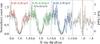 |
Fig. 4 The dip in phase-averaged, energy-resolved X-ray light curves. Left to right: light curves extracted from soft X-ray energy intervals of constant width, compared to the harder 0.5−10.0 keV band. The data are binned into a time resolution of 150 s and normalized to their nondip median count rates. Right panel: corresponding ratios of X-ray soft to X-ray hard light curves, binned into a time resolution of 300 s. |
4.1. The black-body-like component
The soft X-ray component is fitted by an absorbed single-temperature black body at a temperature of  . The tbnew absorption term of
  stays below the upper limit of interstellar hydrogen absorption on our line of sight, NH = 1.2 − 1.6 × 1020 cm-2 (Kalberla et al. 2005; Dickey & Lockman 1990). Using a mekal component for the harder part of the spectrum (cf. Sect. 4.2), we achieve a reduced
  of 1.23 at 199 degrees of freedom over the whole XMM-Newton energy range. Residuals remain around the energies of the emission lines of helium-like C V, N VI, and O VII (Fig. 5).
Single-temperature models approximate a time and spatially averaged temperature of a rather complex accretion area, which is expected to be extended, comprising a wider spread of temperatures, and not necessarily circular (cf. Milgrom & Salpeter 1975; Kuijpers & Pringle 1982; Ferrario & Wickramasinghe 1990). Aiming at a better description of the temperature gradient in the accretion region on the white dwarf, we tested multitemperature black-body models. A fit with a second black body shows that the resolution of the data allows for the application of multicomponent models. It results in a reduced of 1.22 (197 d.o.f., mekal plasma component) and an F-test probability of 75% that the fit is improved. In the fits with multiple black bodies, we employed models that have been successfully used for other polars: black-body components whose effective emitting surface areas obey an exponential distribution over temperatures (AM Her, Beuermann et al. 2012) or whose individual temperatures obey a Gaussian distribution over emitting radii (AI Tri, Traulsen et al. 2010). The model with a Gaussian temperature distribution reproduces the low-energy continuum better, without changing the reduced  over the full 0.1 − 10.0 keV range.
Best-fit parameters for the non-dip EPIC spectra of RS Cae, employing single-temperature components tbnew(bbody+ plasma).
 |
Fig. 5 Nondip EPIC spectra of RS Cae and the xspec black-body plus plasma fits. Small panel: corresponding unabsorbed model fluxes. |
To test the quality of the fits independently of the χ2 fit statistics, we performed a runs test for randomness for each model and determined the probability that the residuals of the fit are randomly distributed around zero. It increases from Prandom = 35% for the single-temperature black body to 45% for the two black-body components and to 76% for the Gaussian temperature distribution, mainly triggered by a low number of residuals changing sign and indicating a somewhat higher preference for the multitemperature approach5. It yields temperatures up to  with highest flux at 34.5 eV and an interstellar absorption term of
 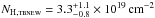 . Owing to the wider temperature range covered, the bolometric model flux
  is about 50% higher than for the single temperature.
4.2. The plasma component
The hard X-ray component is fitted by a mekal plasma model (cf. Mewe et al. 1985; Liedahl et al. 1995), comprising continuum and line emission. Table 2 summarizes the parameters of our three main mekal fits, which we now describe. The pure mekal model is not sufficient to reproduce the observed iron emission around 6.7 keV. Underestimating the continuum flux, it results in an unrealistically high element abundance of several times the solar values. We include a partially covering absorber pcfabs as the simplest approach to the complex absorption spectrum expected for the accretion emission (cf. Done & Magdziarz 1998; Cropper et al. 1998). The best fit yields a mean plasma temperature of  at solar element abundances and intrinsic absorption of
  , covering
  of the emission region. The bolometric model flux of the mekal component increases by a factor of about three when adding the absorption term, as obvious from the plot of the unabsorbed model components in Fig. 5.
In addition, we test the spectra for a neutral Compton reflection component. Reflection features were detected, for example, by Beardmore et al. (1995) for AM Her, by Done & Magdziarz (1998) for BY Cam, or by Bernardini et al. (2012) for hard X-ray selected polars, and theoretically investigated by van Teeseling et al. (1996); Matt (2004); McNamara et al. (2008). In the EPIC spectra of RS Cae, there is no direct evidence of a Fe Kα fluorescent line at 6.4 keV, since the components of the line complex are not resolved. We find an upper limit on the order of 2 × 10⁻⁵ photons cm-2 s-1 in a Gaussian emission line component at 6.4 keV. To test for a reflection continuum, we employed the model by Nandra et al. (2007), developed for Compton reflection by neutral gas in AGN with a power law as incident spectrum, which is based on a model by Magdziarz & Zdziarski (1995) and implemented as pexmon in xspec. A higher runs-test probability of Prandom = 56%, compared to 38% for bbody+pcfabs(mekal), indicates that a reflection component might be present.
As described for the accretion region on the white dwarf, a physically realistic model for the post-shock accretion column needs to include its temperature, density, and velocity structure (cf. Cropper et al. 1999; Fischer & Beuermann 2001). We are employing multitemperature accretion-column models that are based on the models of Fischer & Beuermann (2001) and described by Traulsen et al. (2010) for AI Tri. They fit the spectra of RS Cae well, without improving the χ2 statistical values of the fit significantly. We refer to them in the discussion of the energy balance in Sect. 6. Models with a magnetic field strength of B = 36 MG (Burwitz et al. 1996) and different specific mass flow rates ṁ result in similar values of reduced  to the single-temperature models, but different probabilities Prandom in the runs test for randomness. Best fits are reached for ṁ = 5−10 g cm-2 s-1 in combination with the single-temperature black body at Prandom = 68%, and for ṁ = 0.1 g cm-2 s-1 in combination with the multitemperature black bodies at a high Prandom = 89%. This multi-black body and mekal best-fit model results in essentially the same black-body temperatures as described in Sect. 4.1 and a wide range of plasma temperatures between 2.6 and 62 keV with a flux-weighted mean of
  at a total unabsorbed flux of
  and higher intrinsic absorption of
  .
.
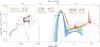 |
Fig. 6 Spectral energy distribution of RS Cae during high and low states of accretion from 1992 to 2010: archival data of various missions from the infrared to the X-ray bands and our 2009 observations. The optical and UV spectroscopic and photometric data are given as orbital minimum and maximum, and 2MASS H- and K-band fluxes as upper limits. The X-ray spectra are shown with the models (solid lines) and their components (dashed and dotted). The shaded areas mark the confidence ranges of the ROSAT temperatures. The gray lines represent stellar and cyclotron model spectra (light gray), and their sum (dark gray, details are given in the text). |
5. Towards a combined SED model
5.1. The spectral energy distribution
Aiming for a physically realistic description of the whole system, we inspected the SED of RS Cae and studied the contributions of the individual system components over the whole energy range. Figure 6 shows the SED in a synopsis of high- and low state observations between 1992 and 2010, including our SMARTS and XMM-Newton data. The ROSAT/WFC count rates of Pye et al. (1995) have been converted into fluxes using the conversion factors according to Hodgkin & Pye (1994), and the EUVE Survey data according to Bowyer et al. (1996). From the first XMM-Newton observation in 2002, obtained during a low state of the system, the Optical-Monitor measurements are included in the plot, while RS Cae was too faint to be detected by the EPIC and RGS instruments (observation ID 0109464301, Ramsay et al. 2004). Since it has low infrared and optical fluxes even during high states of accretion, the WISE data are low signal-to-noise data taken from the reject catalog, and the 2MASS data are “B” quality data (detection valid to 80% − 90%). The survey data (WISE, 2MASS, EUVE, WFC) are snapshots of RS Cae at unknown orbital phase, while the ESO, SMARTS, and XMM-Newton/OM fluxes are given as orbital minimum and maximum during high states and as orbital means during low states. The X-ray spectra are shown unfolded with their respective best-fit models: the XMM-Newton/EPIC data with the absorbed black-body plus mekal fit as described in Sect. 4, and the archival PSPC data with black-body plus bremsstrahlung fits. With the bremsstrahlung temperature being fixed to kTbrems: = 5 keV, they yield  ,
,  for the 1992 January data and
  ,
,  for the 1992 September data. These values are mostly independent of the bremsstrahlung temperature, varying only on a sub-percent level within an 1 − 20 keV interval of kTbrems, but poorly constrained.
We compare the observed data points with models for the different system components and theoretical expectations.
5.2. Spectral models and parameters
In addition to our X-ray spectral fits, we apply three models for the cooler emission in the infrared to the ultraviolet range:
-
(i)
emission from the secondary M-dwarf atmosphere,
-
(ii)
cyclotron emission from the cooling post-shock accretion flow, and
-
(iii)
emission from the unheated white-dwarf atmosphere.
The spectral contribution of the preshock accretion stream is not considered in the plot. We include
-
(i)
a PHOENIX model (Hauschildt &Baron 1999), as employed by Helleret al. (2011) in their analyses ofwhite-dwarf M-star binaries. It depends on temperature, surfacegravity, and chemical composition of the M-dwarf;
-
(ii)
a cyclotron model spectrum by Fischer & Beuermann (2001). It depends on the magnetic field strength, the mass of the white dwarf, and the local mass-flow densities in the accretion column; and
-
(iii)
a non-LTE model atmosphere of a hydrogen-helium white dwarf, using routines of the Tübingen NLTE Model-Atmosphere Package (Werner 1986; Werner & Dreizler 1999). It depends on temperature, surface gravity (or: mass and age), and chemical composition of the white dwarf.
In the following, we describe the parameter set we use for the three models.
Parameters that are constant in time are taken from the literature. For the system geometry, we assume a binary inclination i ~ 60° and a colatitude β ~ 25° of the accretion region on the white dwarf, following the stream-eclipse scenario of Burwitz et al. (1996). For the secondary star (i), we estimate the parameters via the empirical relations by Knigge (2006, 2007) for Porb = 1.7 h: the effective temperature to Teff,2 = 3000 K, the surface gravity to log g2 = 5.0 [cm s-2], and the radius to R2 = 0.166 R⊙. For the white dwarf (ii and iii), we use the magnetic field strength B = 36 MG of Burwitz et al. (1996) and typical values of white dwarfs in polars as reviewed, for example, by Sion (1999); Kawka et al. (2007); Townsley & Gänsicke (2009): Teff,WD = 15 000 K, log gWD = 8.0 [cm s-2], and MWD = 0.6 M⊙, corresponding to a radius of about RWD ~ 0.012 R⊙ (Koester & Schoenberner 1986). In all models, we assume solar element abundances.
The distance to the system cannot be derived directly from the optical spectra, because they lack the features of the secondary star. The models (i to iii) are fully consistent with the ultraviolet, optical, and infrared measurements shown in Fig. 6 if we scale them to a distance of 750 pc. At this value, the M-star model coincides with the ground-based JHK measurements, which serve as an upper limit for the stellar contribution and, thus, as lower limit for the distance estimate. The low J-to-H magnitude ratio supports the interpretation that the 2008 data are M-star-dominated and represent a low state of accretion, while the steeper 2MASS measurements include significant cyclotron emission during a high state. The 750 pc agree with the lower limit of 440 pc given by Burwitz et al. (1996) and with the determination of  of Pretorius et al. (2013). It mainly depends on the stellar radii of the white dwarf and the M-star. A distance less than 750 pc would require smaller radii for both stars in order not to exceed the data; a longer distance would require larger stellar radii to match the observed data. These radii would conflict with the empirical values of Knigge (2006).
Time-variable parameters are mass-flow rates, accretion temperatures, and emitting areas. They have to be fitted per observational epoch. X-ray temperatures, emitting surface areas, and column densities are derived from the X-ray spectral fits (Sects. 4 and 5.1). The mass-flow density in the accretion column is a free parameter of the models of Fischer & Beuermann (2001). We estimate it by scaling the models to approximately match the shape of the ESO spectra observed in 1993: two local mass-flow densities in the accretion column, ṁ1 = 0.01 g cm-2 s-1 with a column base area A1 = 1016 cm2 and ṁ2 = 0.1 g cm-2 s-1 with A2 = 1.3 × 1015 cm2. The bremsstrahlung flux of the Fischer & Beuermann (2001) models are also in accordance with the hard X-ray fluxes in the XMM-Newton/EPIC observation and their upper limits in the ROSAT/PSPC observations, when using a partially covering absorber on the same order as in the spectral fits in Sect. 4.
5.3. Application to the multiband light curves
From the combined spectral models, we derived model light curves in optical, ultraviolet, and soft X-ray bands, aiming at a physical interpretation of the light curves and a consistency check for our models. This is the first effort to model the multiwavelength light curves of a polar, combining photometric with spectroscopic information during high and low states of accretion. For simulating the low-energy light curves, we consider cyclotron emission from the accretion column, accretion-stream emission, and white-dwarf emission. The contribution of the secondary star is negligible in the wave bands of our photometry (cf. Fig. 6).
We calculate the cyclotron light curves from the phase-resolved column spectra (model ii in Sect. 5.2), folding them with the transmission curves of the Johnson-Cousins and XMM-Newton/OM filters. They show a double-humped structure that has been observed and attributed to cyclotron beaming in other polars, as in AM Her (Gänsicke et al. 2001), AR UMa (Howell et al. 2001), and HU Aqr (Schwope et al. 2003). In our models, the phasing of the deepest minimum changes from ϕX − ray = 0.0 in the infrared, U, and B light curves to ϕX − ray = 0.5 in the VRI light curves. The white-dwarf fluxes are given by the atmosphere model (iii) of Sect. 5.2. The flux modulation of the preshock accretion stream with the orbital phase is calculated within a 3D binary model for a constant temperature along the stream (Staude et al. 2001), which means the same relative stream-flux modulation in all filters. The absolute stream flux is guessed per filter from the light curve minima as measured flux minus cyclotron and white-dwarf flux.
To combine the different light curve components, we need their relative phasing, i. e., information on the system geometry. The spectroscopic ephemeris is not accurate enough to be extrapolated to 2009 and to independently determine the orbital phasing. We therefore estimate the phase shifts between the components directly from the observed light curves: the shift between X-ray (dip) phase and cyclotron (magnetic) phase from the primary optical light-curve minimum to ϕX − ray − ϕcycl ~ −0.04, and the shift between cyclotron and stream flux via the color dependence of the secondary minimum and the asymmetric shape of the optical and UV light curves to ϕcycl − ϕstream ~ −0.055. Figure 7 shows our 2009 UVW1, U, and B observations, along with the final simulations.
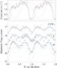 |
Fig. 7 Observed (2009) and simulated light curves of RS Cae. Upper panel: phase-averaged soft X-ray light curve in the black-body-dominated 0.1 keV ≤ E ≤ 0.5 keV band plus simulated light curves of a flat circular (dashed green) and a cylindrical (red) accretion region. The solid curve includes the absorption-dip fit described in the text. EPIC/pn time bins are 100 s. Lower panel: optical monitor UVW1 filter (shifted by − 0.7 mag), U filter, and SMARTS B-band. The dashed and dotted lines represent the cyclotron and the accretion-stream contribution to the B-band simulation, respectively. OM time bins are 300 s. |
In addition, we model the soft X-ray light curves as orbital projections of emitting black-body surface areas, to which the measured black-body flux is proportional. We employ the same binary inclination i ~ 60° and colatitude β ~ 25° of the accretion region as in Sect. 5.2. We start with the simplest approach of a flat circular accretion region (Fig. 7), which results in a significantly higher light-curve amplitude than measured for RS Cae. The observed amplitude could only be explained by a flat emission region if both inclination i and colatitude β were on the order of 25°, which is inconsistent with the optical data of Burwitz et al. (1996). In fact, the soft X-ray and EUV emitting regions are expected to be bulging and arc-shaped rather than flat and circular, corresponding to extended, arc-shaped bases of the post-shock accretion columns (cf. Cropper 1989; Ferrario & Wickramasinghe 1990; Potter et al. 1997). Observationally, evidence of more complexity was found, for example, by Vennes et al. (1995); Sirk & Howell (1998); Gänsicke et al. (1998); Szkody et al. (1999). We tested for a three-dimensional shape of the accretion region of RS Cae with the projection of a cylindrical emission region. The flux from an extended cylinder with a height of 1.25 times its diameter reproduces the soft EPIC/pn light curve reasonably well (Fig. 7). We derive a phase shift of about ϕX − ray − ϕsoftX ~ − 0.2 from the light curves, where ϕsoftX denotes maximum soft X-ray flux, i.e., maximum visibility of the accretion region. This shift means that the centers of accretion region and accretion column might be offset.
To account for the stream-absorption dip in our simulations of the soft X-ray light curves, we use phase-resolved spectral models of the dip phase. We extract EPIC/pn spectra at energies below 0.5 keV in a ± 0.225 phase range around the dip center with a phase resolution of Δϕ = 0.05 and fit them simultaneously with absorbed black-body models. Since the Δϕ = 0.05 spectra during dip phase comprise only a few bins, we repeat the fit with spectra extracted for overlapping Δϕ = 0.1 intervals, centered at ϕX − ray = 0.00,0.05,0.10, etc., similar to the approach that Girish et al. (2007) use to fit the iron lines of AM Her. We use identical black-body temperatures for all phase intervals and couple the normalizations (i.e., emitting surface areas) according to the projected areas of the cylindrical emission region. The hydrogen absorption on the line of sight increases in our fits up to NH,tbabs ~ 8 × 1022 cm-2, including interstellar absorption, during the dip phase. With a reduced  of the simultaneous black-body fit, modeling the emission region as a three-dimensional cylinder is significantly more appropriate than as a flat circle, but still lacking. We convert the Δϕ = 0.05 model fluxes in the 0.1 − 0.5 keV interval to absorption factors by dividing the absorbed fluxes by the fluxes for a constant interstellar (nondip) absorption of NH = 2.1 × 1019 cm-2 and multiply the simulated X-ray light curves by them. The results are shown in the upper panel of Fig. 7 and give a reasonable description of the absorption dip. Deficits of the model manifest themselves in particular between ϕX − ray = 0.1 and 0.2, where the count rate is underestimated because of the simplifications made in modeling the emitting areas and the phase shifts.
5.4. Results
With our SED and light curve models, we separate the contributions of the different system components to the SED and derive a new lower limit estimate of the distance to RS Cae. In the infrared range, a large part of the total flux can be attributed to the M-type secondary, plus cyclotron emission during high states of accretion. The cyclotron component is dominating the stellar emission in the optical and near-infrared range. In particular, large parts of the B-band modulation can be attributed to cyclotron emission (Fig. 7). The color dependence of the light-curve minima is explained by the decreasing contribution of the cyclotron flux and increasing contribution of accretion-stream flux from the optical toward the ultraviolet. The cyclotron model spectra reproduce the high-state data in 1993 and 2009, and the 2MASS data indicate that even higher infrared fluxes may be reached at other epochs. The unheated white dwarf contributes little to the high-state flux, with the low-state UV flux serving as upper limit for the white dwarf.
6. The energy balance of RS Cae
Since RS Cae was discovered at a hardness ratio close to − 1.0 during the ROSAT All-Sky Survey (Thomas et al. 1998), it has been considered to be one of the soft X-ray dominated polars. In these systems, the soft X-ray luminosity exceeds the 50% of the total luminosity predicted by the standard model of accretion (King & Lasota 1979; Lamb & Masters 1979). Former ROSAT results are biased towards soft energies, since the energy range was limited to 0.1 − 2.5 keV, and have to be verified over a broader energy range. With our fits to the XMM-Newton spectra, we investigate the energy balance of RS Cae on the basis of data in the 0.1 − 0.5 keV and 0.5 − 10.0 keV bands, and with our SED models on the basis of the optical and ultraviolet measurements.
6.1. XMM-Newton fluxes and X-ray flux ratios
From the absorbed single-temperature model described in Sect. 4, we have derived bolometric fluxes of Fbol(bbody) =  and Fbol(mekal) =
  , and a soft-to-hard flux ratio of
  during non-dip phases. For the cyclotron component, we estimate a bolometric flux of about Fbol,cycl ~ 5 × 10-13 erg cm-2 s-1 from the accretion-column model presented in Sect. 5.2.
The flux values strongly depend on the choice of the spectral model (cf. Table 2). Ramsay & Cropper (2004) present flux and luminosity ratios based on single-temperature black-body and multitemperature column models. Multitemperature models typically result in higher bolometric fluxes: since the flux in the instrumental energy window is scaled to the observed flux, the fluxes toward the (unobserved) lower and higher energies are raised compared to a single-temperature continuum owing to the broader temperature range (cf. small panel in Fig. 5). Our fits indicate that the spectra reflect the multitemperature nature both of accretion region and accretion column, while higher spectral resolution and sensitivity would be needed to derive the parameter distributions directly from the observed data. In the combined multicomponent fit with predefined temperature distributions, the bolometric fluxes of both the multi-bbodyrad and the multi-mekal component increase by a factor of 1.5, respectively, leaving the flux ratio essentially unchanged.
The soft X-ray excess of polars that was measured from ROSAT data increases with magnetic field strength (Beuermann & Schwope 1994; Ramsay et al. 1994). The excess in RS Cae is comparable to the XMM-Newton results for polars of similar field strengths: EK UMa (B ~ 35 MG) with a moderate luminosity ratio of six for single-temperature models during a short 5 ks exposure (Ramsay & Cropper 2004); AI Tri (B ~ 38 MG) with moderate to high flux ratios of 6 to at least 70, depending on the accretion state (Traulsen et al. 2010); HU Aqr (B ~ 35 MG) with low flux ratios during a low state of accretion, balanced fluxes or a slight excess during an intermediate state, and a strong excess during a high state (Schwarz et al. 2009).
6.2. XMM-Newton and optical luminosities
We convert the bolometric fluxes to luminosities as L = ηπFd2, where η denotes the geometric correction factor. Typically, for the hard component a factor of 3π (considering reflection effects) up to 4π is chosen, while King & Watson (1987) emphasize that a factor of 2π for column emission into one half space would be more appropriate. For the soft emission of a flat accretion region, a factor of 2π or πcos-1ϑ, depending on the viewing angle ϑ, is used, and of 4π for blobby accretion when accretion mounds form at the impact area due to the heating of the photosphere (Hameury & King 1988; Beuermann & Schwope 1989). Having shown the evidence of a three-dimensional structure of the accretion region in RS Cae, we choose the same geometric factor of 4π for the X-ray soft and for the X-ray hard component, and 2π for the cyclotron component. For the multitemperature model, we thus obtain LsoftX = 7.7 × 1032 erg s-1, LhardX = 7.3 × 1031 erg s-1, Lcycl ~ 1.7 × 1031 erg s-1 for a distance of d = 750 pc, and soft-to-hard luminosity ratios on the same order of 10 as the flux ratios.
The accretion-induced luminosities of soft X-ray, hard X-ray, and cyclotron component add to Laccr = 8.6 × 1032 erg s-1, without the (unknown) contribution of the preshock accretion stream. For a white-dwarf mass of MWD = 0.6 M⊙ and radius of RWD ~ 0.012 R⊙, this corresponds to a mass-accretion rate on the order of Ṁ = Laccr RWD/(G MWD) ~ 10-10 M⊙ yr-1, within the typical range of high-state accretion rates of polars.
6.3. Long-term characteristics of soft and hard emission
The SED plot in Fig. 6 shows the distinct soft X-ray components in the ROSAT and XMM-Newton observations. They changed significantly from 1992 to 2009, seen in the emitting black-body areas, which represent the area at the mean temperature of the accretion region, and, correspondingly, in the (bolometric) fluxes of the black-body fits (Table 3): the soft X-ray fluxes during the ROSAT observation of September 1992 are by a factor of at least 5.5 higher than during the 2009 XMM-Newton observation. The hard X-ray and cyclotron fluxes, on the other hand, are on the same order of magnitude during the 2009 observations as in 1992/93. Both hard X-ray and cyclotron emission are assumed to arise from the accretion column, so the similar flux levels may indicate similar physical properties of the column at both epochs. Although the ROSAT fit results are poorly constrained, they show clearly that the long-term characteristics of soft and hard X-ray component are not correlated. Gänsicke et al. (1995) demonstrated for AM Her that the bremsstrahlung and cyclotron flux are balanced by the (reprocessed) UV flux both during high and low states of accretion, independently of the soft X-ray component, which arises from blobby accretion. Correspondingly, the soft stages of RS Cae and its decoupled soft and hard X-ray fluxes may indicate inhomogeneous accretion processes.
Emitting black-body areas and bolometric fluxes of RS Cae during the high-state observations by ROSAT in 1992 and XMM-Newton in 2009, together with their 90% confidence intervals.
7. Summary and conclusions
Our pointed XMM-Newton observation of RS Cae, covering 4.5 orbital cycles, provides the first opportunity to investigate its energy balance on the basis of data at energies up to 10 keV. RS Cae was clearly in a high state of accretion at the epoch of our observations. Archival infrared and X-ray data indicated that still higher and potentially softer states might be possible. Almost 97% of the EPIC/pn photons were detected in the soft range, yielding hardness ratios close to − 1 in the X-ray light curves. The light curves gave evidence of a three-dimensional shape of the accretion region and inhomogeneous accretion events, as is typical of soft polars. We identified the sharp, recurring light-curve dips as stream absorption and used them to derive a photometric period of 0.0709(3) days, confirming the preferred period of Burwitz et al. (1996) and placing RS Cae among the short-period polars. The energy dependence of the width of the dip, becoming broader towards higher energies, indicated different spatial extents of the X-ray emitting regions.
Using SED modeling, we consistently connected the multiwavelength spectra and light curves of the different system components. SEDs constructed of nonsimultaneous observations provide insight into long-term behavior and accretion-stage changes in the system, but have a limited ability to model the SED. This successful approach shows the potential of SED modeling and simultaneous multiwavelength observations of polars.
Using single- and multitemperature fits to the EPIC spectra, we find a soft X-ray excess with soft-to-hard luminosity ratios of about ten. Our multitemperature spectral models give physically plausible descriptions of the structure of the accretion region and column and the respective X-ray and low-energy spectra and light curves. They result in the same soft-to-hard flux ratios as the single-temperature models.
Up to now, we have studied three systems with a clear soft X-ray excess during (intermediate) high states of accretion in the ROSAT and in our pointed XMM-Newton observations: AI Tri (Traulsen et al. 2010), QS Tel (Traulsen et al. 2011), and RS Cae. Their soft X-ray luminosity correlates with their accretion state and can change drastically on time scales as short as days, in agreement with the dependence of the soft-to-hard luminosity ratio on the accretion state as described by Ramsay & Cropper (2004). The three systems augment the number of polars whose ROSAT-detected soft X-ray excess could be confirmed over the broader energy range of XMM-Newton. Which fraction of AM Her-type systems actually shows a soft X-ray excess is hard to determine from the currently available data. One limiting factor has been instrumental biases. With higher sensitivity in particular in the hard X-ray regime, an increasing number of X-ray hard and low accretion rate polars are being detected. Another limiting factor is observational biases. In untriggered observations, a substantial number of polars are caught during low states, so their soft stages would be missed. Considering the selection effects and our observational results, we expect that the fraction of 25% X-ray soft polars among ROSAT detections might overestimate the actual number, but that the soft systems form a significant group among the polars.
Hardness ratio HR1ROSAT = (HR − SR)/(HR + SR) of count rates in the 0.1−0.5 keV (SR) and 0.5−2.5 keV (HR) energy bands, respectively.
Maximum rate and Poissonian error derived from 1 ks light-curve segments.
Corrected count rates and errors given by the OM source-detection tasks.
Most recent version of tbvarabs in xspec. See http://pulsar.sternwarte.uni-erlangen.de/wilms/research/tbabs/
Probabilities of the two-tailed runs test have been calculated as twice the single-tail values of a normalized Normal distribution. If the data are described well by the model, we expect a random distribution, while systematic deviations manifest themselves as longer sequences of positive or of negative residuals and a lower probability value.
Acknowledgments
This research has been supported by the DLR under project numbers 50 OR 0501, 50 OR 0807, and 50 OR 1011. We thank René Heller for providing the M-star spectrum shown in Fig. 6 and Karleyne Silva for calculating accretion-column light curves and for fruitful discussions. FWM’s access to the SMARTS observatory is supported in part by a NASA grant NNX10AE51G to Stony Brook University. Figure 6 includes data from the High Energy Astrophysics Science Archive Research Center (HEASARC), provided by NASA’s Goddard Space Flight Center; data products from the Two Micron All Sky Survey, which is a joint project of the University of Massachusetts and the Infrared Processing and Analysis Center/California Institute of Technology, funded by the National Aeronautics and Space Administration and the National Science Foundation; and data products from the Wide-field Infrared Survey Explorer, which is a joint project of the University of California, Los Angeles, and the Jet Propulsion Laboratory/California Institute of Technology, funded by the National Aeronautics and Space Administration.
References
- Arnaud, K. A. 1996, in Astronomical Data Analysis Software and Systems V, eds. G. H. Jacoby & J. Barnes, ASP Conf. Ser., 101, 17 [Google Scholar]
- Asplund, M., Grevesse, N., Sauval, A. J., & Scott, P. 2009, ARA&A, 47, 481 [NASA ADS] [CrossRef] [Google Scholar]
- Beardmore, A. P., Done, C., Osborne, J. P., & Ishida, M. 1995, MNRAS, 272, 749 [NASA ADS] [Google Scholar]
- Bernardini, F., de Martino, D., Falanga, M., et al. 2012, A&A, 542, A22 [NASA ADS] [CrossRef] [EDP Sciences] [Google Scholar]
- Beuermann, K., & Burwitz, V. 1995, in Magnetic Cataclysmic Variables, eds. D. A. H. Buckley & B. Warner, ASP Conf. Ser., 85, 99 [Google Scholar]
- Beuermann, K., & Schwope, A. D. 1989, A&A, 223, 179 [NASA ADS] [Google Scholar]
- Beuermann, K., & Schwope, A. D. 1994, in Interacting Binary Stars, ed. A. W. Shafter, ASP Conf. Ser., 56, 119 [Google Scholar]
- Beuermann, K., Thomas, H.-C., Reinsch, K., et al. 1999, A&A, 347, 47 [NASA ADS] [Google Scholar]
- Beuermann, K., Burwitz, V., & Reinsch, K. 2012, A&A, 543, A41 [NASA ADS] [CrossRef] [EDP Sciences] [Google Scholar]
- Bowyer, S., Lieu, R., Lampton, M., et al. 1994, ApJS, 93, 569 [NASA ADS] [CrossRef] [Google Scholar]
- Bowyer, S., Lampton, M., Lewis, J., et al. 1996, ApJS, 102, 129 [NASA ADS] [CrossRef] [Google Scholar]
- Burwitz, V., Reinsch, K., Schwope, A. D., et al. 1996, A&A, 305, 507 [NASA ADS] [Google Scholar]
- Cropper, M. 1989, MNRAS, 236, 935 [NASA ADS] [Google Scholar]
- Cropper, M., Ramsay, G., & Wu, K. 1998, MNRAS, 293, 222 [NASA ADS] [CrossRef] [Google Scholar]
- Cropper, M., Wu, K., Ramsay, G., & Kocabiyik, A. 1999, MNRAS, 306, 684 [NASA ADS] [CrossRef] [Google Scholar]
- Dickey, J. M., & Lockman, F. J. 1990, ARA&A, 28, 215 [NASA ADS] [CrossRef] [MathSciNet] [Google Scholar]
- Done, C., & Magdziarz, P. 1998, MNRAS, 298, 737 [NASA ADS] [CrossRef] [Google Scholar]
- Dorman, B., Arnaud, K. A., & Gordon, C. A. 2003, in Bull. Am. Astron. Soc., 35, 641 [Google Scholar]
- Ferrario, L., & Wickramasinghe, D. T. 1990, ApJ, 357, 582 [NASA ADS] [CrossRef] [Google Scholar]
- Fischer, A., & Beuermann, K. 2001, A&A, 373, 211 [NASA ADS] [CrossRef] [EDP Sciences] [Google Scholar]
- Gänsicke, B. T., Beuermann, K., & de Martino, D. 1995, A&A, 303, 127 [NASA ADS] [Google Scholar]
- Gänsicke, B. T., Hoard, D. W., Beuermann, K., Sion, E. M., & Szkody, P. 1998, A&A, 338, 933 [NASA ADS] [Google Scholar]
- Gänsicke, B. T., Fischer, A., Silvotti, R., & de Martino, D. 2001, A&A, 372, 557 [NASA ADS] [CrossRef] [EDP Sciences] [Google Scholar]
- Gerke, J. R., Howell, S. B., & Walter, F. M. 2006, PASP, 118, 678 [NASA ADS] [CrossRef] [Google Scholar]
- Girish, V., Rana, V. R., & Singh, K. P. 2007, ApJ, 658, 525 [NASA ADS] [CrossRef] [Google Scholar]
- Hameury, J. M., & King, A. R. 1988, MNRAS, 235, 433 [NASA ADS] [Google Scholar]
- Hauschildt, P. H., & Baron, E. 1999, J. Comp. Appl. Math., 109, 41 [Google Scholar]
- Heller, R., Schwope, A. D., & Østensen, R. H. 2011, in Evolution of Compact Binaries, eds. L. Schmidtobreick, M. R. Schreiber, & C. Tappert, ASP Conf. Ser., 447, 177 [Google Scholar]
- Hodgkin, S. T., & Pye, J. P. 1994, MNRAS, 267, 840 [NASA ADS] [Google Scholar]
- Howell, S. B., Gelino, D. M., & Harrison, T. E. 2001, AJ, 121, 482 [NASA ADS] [CrossRef] [Google Scholar]
- Kalberla, P. M. W., Burton, W. B., Hartmann, D., et al. 2005, A&A, 440, 775 [NASA ADS] [CrossRef] [EDP Sciences] [Google Scholar]
- Kawka, A., Vennes, S., Schmidt, G. D., Wickramasinghe, D. T., & Koch, R. 2007, ApJ, 654, 499 [NASA ADS] [CrossRef] [Google Scholar]
- King, A. R., & Lasota, J. P. 1979, MNRAS, 188, 653 [NASA ADS] [CrossRef] [Google Scholar]
- King, A. R., & Watson, M. G. 1987, MNRAS, 227, 205 [NASA ADS] [Google Scholar]
- Knigge, C. 2006, MNRAS, 373, 484 [NASA ADS] [CrossRef] [Google Scholar]
- Knigge, C. 2007, MNRAS, 382, 1982 [NASA ADS] [Google Scholar]
- Koester, D., & Schoenberner, D. 1986, A&A, 154, 125 [NASA ADS] [Google Scholar]
- Kuijpers, J., & Pringle, J. E. 1982, A&A, 114, L4 [NASA ADS] [Google Scholar]
- Lamb, D. Q., & Masters, A. R. 1979, ApJ, 234, L117 [NASA ADS] [CrossRef] [Google Scholar]
- Liedahl, D. A., Osterheld, A. L., & Goldstein, W. H. 1995, ApJ, 438, L115 [NASA ADS] [CrossRef] [Google Scholar]
- Magdziarz, P., & Zdziarski, A. A. 1995, MNRAS, 273, 837 [NASA ADS] [CrossRef] [Google Scholar]
- Matt, G. 2004, A&A, 423, 495 [NASA ADS] [CrossRef] [EDP Sciences] [Google Scholar]
- McNamara, A. L., Kuncic, Z., Wu, K., Galloway, D. K., & Cullen, J. G. 2008, MNRAS, 383, 962 [NASA ADS] [CrossRef] [Google Scholar]
- Mewe, R., Gronenschild, E. H. B. M., & van den Oord, G. H. J. 1985, A&AS, 62, 197 [NASA ADS] [Google Scholar]
- Milgrom, M., & Salpeter, E. E. 1975, ApJ, 196, 583 [NASA ADS] [CrossRef] [Google Scholar]
- Nandra, K., O’Neill, P. M., George, I. M., & Reeves, J. N. 2007, MNRAS, 382, 194 [NASA ADS] [CrossRef] [Google Scholar]
- Potter, S. B., Cropper, M., Mason, K. O., Hough, J. H., & Bailey, J. A. 1997, MNRAS, 285, 82 [NASA ADS] [CrossRef] [Google Scholar]
- Pounds, K. A., Allan, D. J., Barber, C., et al. 1993, MNRAS, 260, 77 [NASA ADS] [Google Scholar]
- Pretorius, M. L., Knigge, C., & Schwope, A. D. 2013, MNRAS, 432, 570 [NASA ADS] [CrossRef] [Google Scholar]
- Pye, J. P., McGale, P. A., Allan, D. J., et al. 1995, MNRAS, 274, 1165 [NASA ADS] [Google Scholar]
- Ramsay, G., & Cropper, M. 2004, MNRAS, 347, 497 [NASA ADS] [CrossRef] [Google Scholar]
- Ramsay, G., Mason, K. O., Cropper, M., Watson, M. G., & Clayton, K. L. 1994, MNRAS, 270, 692 [NASA ADS] [CrossRef] [Google Scholar]
- Ramsay, G., Cropper, M., Wu, K., et al. 2004, MNRAS, 350, 1373 [NASA ADS] [CrossRef] [Google Scholar]
- Schwarz, R., Schwope, A. D., Vogel, J., et al. 2009, A&A, 496, 833 [NASA ADS] [CrossRef] [EDP Sciences] [Google Scholar]
- Schwope, A. D., Brunner, H., Buckley, D., et al. 2002, A&A, 396, 895 [NASA ADS] [CrossRef] [EDP Sciences] [Google Scholar]
- Schwope, A. D., Thomas, H.-C., Mante, K.-H., Haefner, R., & Staude, A. 2003, A&A, 402, 201 [NASA ADS] [CrossRef] [EDP Sciences] [Google Scholar]
- Silva, K. M. G., Rodrigues, C. V., & Costa, J. E. R. 2011 [arXiv:1101.5568] [Google Scholar]
- Sion, E. M. 1999, PASP, 111, 532 [NASA ADS] [CrossRef] [Google Scholar]
- Sirk, M. M., & Howell, S. B. 1998, ApJ, 506, 824 [NASA ADS] [CrossRef] [Google Scholar]
- Standish, E. M. 1998, JPL IOM, 312.F-98-048 [Google Scholar]
- Staude, A., Schwope, A. D., & Schwarz, R. 2001, A&A, 374, 588 [NASA ADS] [CrossRef] [EDP Sciences] [Google Scholar]
- Szkody, P., Vennes, S., Schmidt, G. D., et al. 1999, ApJ, 520, 841 [NASA ADS] [CrossRef] [Google Scholar]
- Thomas, H.-C., Beuermann, K., Reinsch, K., et al. 1998, A&A, 335, 467 [NASA ADS] [Google Scholar]
- Townsley, D. M., & Gänsicke, B. T. 2009, ApJ, 693, 1007 [NASA ADS] [CrossRef] [Google Scholar]
- Traulsen, I., Reinsch, K., Schwarz, R., et al. 2010, A&A, 516, A76 [NASA ADS] [CrossRef] [EDP Sciences] [Google Scholar]
- Traulsen, I., Reinsch, K., Schwope, A. D., et al. 2011, A&A, 529, A116 [NASA ADS] [CrossRef] [EDP Sciences] [Google Scholar]
- van Teeseling, A., Kaastra, J. S., & Heise, J. 1996, A&A, 312, 186 [NASA ADS] [Google Scholar]
- Vennes, S., Szkody, P., Sion, E. M., & Long, K. S. 1995, ApJ, 445, 921 [NASA ADS] [CrossRef] [Google Scholar]
- Verner, D. A., & Ferland, G. J. 1996, ApJS, 103, 467 [NASA ADS] [CrossRef] [Google Scholar]
- Verner, D. A., Ferland, G. J., Korista, K. T., & Yakovlev, D. G. 1996, ApJ, 465, 487 [NASA ADS] [CrossRef] [Google Scholar]
- Voges, W., Aschenbach, B., Boller, T., et al. 1999, A&A, 349, 389 [NASA ADS] [Google Scholar]
- Werner, K. 1986, A&A, 161, 177 [NASA ADS] [Google Scholar]
- Werner, K., & Dreizler, S. 1999, J. Comp. Appl. Math., 109, 65 [Google Scholar]
- Wilms, J., Allen, A., & McCray, R. 2000, ApJ, 542, 914 [NASA ADS] [CrossRef] [Google Scholar]
All Tables
Barycentric timings and 1σ errors of the dip centers in the XMM-Newton light curves of RS Cae.
Best-fit parameters for the non-dip EPIC spectra of RS Cae, employing single-temperature components tbnew(bbody+ plasma).
Emitting black-body areas and bolometric fluxes of RS Cae during the high-state observations by ROSAT in 1992 and XMM-Newton in 2009, together with their 90% confidence intervals.
All Figures
|
Fig. 1 September 2009 light curves of RS Cae in time bins of 100 s, folded on the orbital period with the center of the X-ray dips defining phase zero (Eq. (1)). The grey area marks the interval of high background activity during the XMM-Newton pointing. a)–b) Energy-resolved EPIC/pn light curves. c) Corresponding hardness ratios HRXMM = (HX − SX)/(HX + SX). d) Optical and ultraviolet light curves measured subsequently with three filters at the optical monitor. e) Optical B-band light curve with a time resolution of about 227 s, plotted twice and shifted by − 3 and − 2 orbital cycles, respectively. |
| In the text | |
|
Fig. 2 Phase-averaged X-ray light curves, excluding the high-background interval, in time bins of 60 s and with the same phase convention and energy ranges as in Fig. 1. a–b) Energy-resolved EPIC/pn light curves. c) Corresponding hardness ratios. |
| In the text | |
|
Fig. 3 SMARTS B-band light curves of RS Cae obtained at 2008/09/22 during a low state and at 2009/03/12 during a high state of accretion, each folded on a period of |
| In the text | |
|
Fig. 4 The dip in phase-averaged, energy-resolved X-ray light curves. Left to right: light curves extracted from soft X-ray energy intervals of constant width, compared to the harder 0.5−10.0 keV band. The data are binned into a time resolution of 150 s and normalized to their nondip median count rates. Right panel: corresponding ratios of X-ray soft to X-ray hard light curves, binned into a time resolution of 300 s. |
| In the text | |
|
Fig. 5 Nondip EPIC spectra of RS Cae and the xspec black-body plus plasma fits. Small panel: corresponding unabsorbed model fluxes. |
| In the text | |
|
Fig. 6 Spectral energy distribution of RS Cae during high and low states of accretion from 1992 to 2010: archival data of various missions from the infrared to the X-ray bands and our 2009 observations. The optical and UV spectroscopic and photometric data are given as orbital minimum and maximum, and 2MASS H- and K-band fluxes as upper limits. The X-ray spectra are shown with the models (solid lines) and their components (dashed and dotted). The shaded areas mark the confidence ranges of the ROSAT temperatures. The gray lines represent stellar and cyclotron model spectra (light gray), and their sum (dark gray, details are given in the text). |
| In the text | |
|
Fig. 7 Observed (2009) and simulated light curves of RS Cae. Upper panel: phase-averaged soft X-ray light curve in the black-body-dominated 0.1 keV ≤ E ≤ 0.5 keV band plus simulated light curves of a flat circular (dashed green) and a cylindrical (red) accretion region. The solid curve includes the absorption-dip fit described in the text. EPIC/pn time bins are 100 s. Lower panel: optical monitor UVW1 filter (shifted by − 0.7 mag), U filter, and SMARTS B-band. The dashed and dotted lines represent the cyclotron and the accretion-stream contribution to the B-band simulation, respectively. OM time bins are 300 s. |
| In the text | |
Current usage metrics show cumulative count of Article Views (full-text article views including HTML views, PDF and ePub downloads, according to the available data) and Abstracts Views on Vision4Press platform.
Data correspond to usage on the plateform after 2015. The current usage metrics is available 48-96 hours after online publication and is updated daily on week days.
Initial download of the metrics may take a while.