| Issue |
A&A
Volume 562, February 2014
|
|
|---|---|---|
| Article Number | A52 | |
| Number of page(s) | 19 | |
| Section | Extragalactic astronomy | |
| DOI | https://doi.org/10.1051/0004-6361/201220455 | |
| Published online | 06 February 2014 | |
Lyman α line and continuum radiative transfer in a clumpy interstellar medium
1
Department of AstronomyStockholm University,
Oscar Klein Center, AlbaNova,
106 91
Stockholm,
Sweden
e-mail:
This email address is being protected from spambots. You need JavaScript enabled to view it.
2
Observatoire de Genève, Université de Genève,
51 Ch. des
Maillettes, 1290
Versoix,
Switzerland
3
CNRS, IRAP, 14
avenue E. Belin, 31400
Toulouse,
France
4
Dark Cosmology Centre, Niels Bohr Institute, University of
Copenhagen, Juliane Maries Vej
30, 2100
Cøpenhagen,
Denmark
Received:
27
September
2012
Accepted:
10
May
2013
Abstract
Aims. We study the effects of an inhomogeneous interstellar medium (ISM) on the strength and the shape of the Lyman alpha (Lyα) line in starburst galaxies.
Methods. Using our 3D Monte Carlo Lyα radiation transfer code, we have studied the radiative transfer of Lyα, UV, and optical continuum photons in homogeneous and clumpy shells of neutral hydrogen and dust surrounding a central source. Our simulations predict the Lyα and continuum escape fraction, the Lyα equivalent width EW(Lyα), the Lyα line profile, and their dependence on the geometry of the gas distribution and the main input physical parameters.
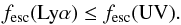
Results. The ISM clumpiness is found to have a strong impact on the Lyα line radiative transfer, leading to a strong dependence of the emergent features of the Lyα line (escape fraction, EW(Lyα)) on the ISM morphology. Although a clumpy and dusty ISM appears more transparent to radiation (both line and continuum) compared to an equivalent homogeneous ISM of equal dust optical depth, we find that the Lyα photons are, in general, still more attenuated than UV continuum radiation. As a consequence, the observed equivalent width of the Lyα line (EWobs(Lyα)) is lower than the intrinsic one (EWint(Lyα)) for nearly all clumpy ISM configurations being considered. There are, however, special conditions under which Lyα photons escape more easily than the continuum, resulting in an enhanced EWobs(Lyα). The requirement for this to happen is that the ISM is almost static (galactic outflows ≤200 km s-1), extremely clumpy (with density contrasts >107 in HI between clumps and the interclump medium), and very dusty (E(B − V) > 0.30). When these conditions are fulfilled, the emergent Lyα line profile generally shows no velocity shift and little asymmetry. Otherwise, the Lyα line profile is very similar to the one expected for homogeneous media.
Conclusions. Given the asymmetry and velocity shifts generally observed in star-forming galaxies with Lyα emission, we therefore conclude that clumping is unlikely to significantly enhance their relative Lyα/UV transmission.
Key words: galaxies: starburst / galaxies: ISM / galaxies: high-redshift / ultraviolet: galaxies / radiative transfer / line: profiles
© ESO, 2014
1. Introduction
As the intrinsically brightest spectral signature of remote young galaxies (Partridge & Peebles 1967; Schaerer 2003), and because it possesses a rest wavelength of 1216 Å that makes it accessible to optical/near-infrared ground-based telescopes for redshifts z ≥ 2, the Lyman alpha (Lyα) line has become the most powerful emission-line probe of the distant young universe. The potential of the Lyα emission line for detection and redshift confirmation of distant galaxies, for derivation of the star formation rate (SFR), and for probing the ionization state of the intergalactic medium (IGM; Malhotra & Rhoads 2004; Kashikawa et al. 2006) and the reionization epoch (Fan et al. 2002; Santos 2004) is enormous, but necessarily relies on a good astrophysical understanding of the processes that regulate the emergent Lyα emission from a galaxy.
The importance of the Lyα line in the cosmological context was first proposed by Partridge & Peebles (1967), who suggested that young high-z galaxies, which are undergoing their first star-forming event, should be detectable thanks to their strong Lyα emission line. Unfortunately, the first attempts to detect high-redshift galaxies in Lyα gave quite meager results. The observed Lyα fluxes appeared fainter than those predicted, and only a few Lyα emitters (LAEs) had been detected until the late 1990 s (cf. Djorgovski & Thompson 1992; Pritchet 1994). This lack of Lyα emission has nevertheless triggered several studies that have highlighted the high complexity of the resonant Lyα line radiative transfer in starburst galaxies (Meier & Terlevich 1981; Neufeld 1990; Charlot & Fall 1993; Kunth et al. 1998; Tenorio-Tagle et al. 1999; Mas-Hesse et al. 2003; Östlin et al. 2009). While the faint measured Lyα fluxes were originally attributed to the dust attenuation (Pritchet 1994), it has turned out that many physical effects could strongly modify or suppress the Lyα line within galaxies (metallicity, neutral hydrogen kinematics, geometry of the interstellar medium – ISM). It is only during this past decade, and after the development of deep and wide surveys, that many Lyα-emitting galaxies have been detected (Hu et al. 1998, 2004; Cowie & Hu 1998; Kudritzki et al. 2000; Rhoads et al. 2000; Taniguchi et al. 2003, 2005; Shimasaku et al. 2006; Gronwall et al. 2007; Nilsson et al. 2007; Guaita et al. 2010; Ouchi et al. 2003, 2008, 2010).
Because of the factors that contribute to the Lyα radiative transfer, the Lyα line features (line profile, equivalent width EW(Lyα), offset from other emission/absorption lines) encode much information on the properties of individual galaxies: gas kinematics, gas geometry, and stellar population. For instance, the detection of unusually strong Lyα line in the spectra of high-z galaxies could indicate the presence of population III stars within them (Schaerer 2003), whereas the asymmetry of the line profiles would suggest the presence of strong galactic outflows (Kunth et al. 1998). The derivation of this precious information, however, requires an accurate interpretation of the Lyα line features, which also implies a complete understanding of the Lyα radiative transfer in the ISM of galaxies. This is one of the aims of this paper.
Owing to the importance of the Lyα line for cosmology, several studies have attempted to understand the physical process governing the escape of Lyα photons from galaxies. Among the parameters that influence the visibility of the Lyα line, the dust content, neutral gas kinematics, and the geometry of the neutral gas seem to play the most important roles. Dust was originally invoked to explain the absence or the faint Lyα emission from galaxies at high redshift (e.g. Meier & Terlevich 1981). However, Giavalisco et al. (1996) studied a local sample of star-forming galaxies observed with the IUE space telescope and found no clear correlation between Lyα/Hβ or EW(Lyα) and the reddening E(B − V).
Other studies have also led to a lack of correlation between the dust attenuation and the strength of the Lyα line, suggesting that other parameters govern the escape of Lyα photons (Kunth et al. 1994; Thuan et al. 1997; Atek et al. 2008). Among them, the role of the neutral gas kinematics was revealed in the 1990 s by Kunth et al. (1994) and Lequeux et al. (1995). For eight local galaxies observed with the Goddard High Resolution Spectrograph (GHRS), Kunth et al. (1998) found that when Lyα line appeared in emission, there was a systematic blueshift of low ionization states (LIS) metal absorption lines with respect to Lyα, indicative of outflows in the neutral medium. Furthermore, the shape of the Lyα line profiles proved to be asymmetric. Galaxies showing Lyα in absorption showed significantly smaller relative shifts of LIS lines and Lyα. This result clearly shows that the Lyα escape fraction and line shape are strongly affected by the kinematical configuration in the ISM. Phenomenologically it is easy to understand that an outflow in the neutral ISM would promote the escape of Lyα photons and create asymmetric line profiles, since the motion Doppler shifts the line out of resonance and more so for the red side of the line. Finally, several studies of the resonant Lyα transfer have emphasized the importance of the ISM clumpiness on the escape of the Lyα (Neufeld 1991; Giavalisco et al. 1996). In particular, Neufeld (1991) showed that it could be possible to observe an emergent EW(Lyα) higher than the intrinsic one in a dusty and clumpy ISM. Since the clumpiness of the ISM is well established in our galaxy (Stutzki & Guesten 1990; Marscher et al. 1993), this parameter must therefore be taken into account in the study of the Lyα radiative transfer.
With the increased number of Lyα radiative transfer codes developed recently (Ahn et al. 2001, 2002; Cantalupo et al. 2005; Verhamme et al. 2006; Pierleoni et al. 2007; Laursen et al. 2009a; Forero-Romero et al. 2011), the transfer of Lyα photons has intensively been investigated in the framework of galaxy simulations. In particular, such simulations allow us to compare the observed Lyα line properties of individual galaxies, both nearby and distant ones (Ahn et al. 2003; Verhamme et al. 2008; Atek et al. 2009). However, although most studies have treated the Lyα radiative transfer in either static or expanding media, the main effects of a multiphase ISM on the Lyα radiative transfer has been the object of a few numerical studies (Haiman & Spaans 1999; Richling 2003; Hansen & Oh 2006; Laursen et al. 2013). The aim of this paper is to carry out a detailed study of both the Lyα and the UV continuum radiative transfer in a wide range of dusty, moving, homogeneous, and clumpy ISMs. This will allow us to examine the effects of the ISM clumpiness on the features of the Lyα line in detail (Lyα escape fraction, EW(Lyα), Lyα line profiles).
One of the main motivations of our study is also to understand the anomalously strong EW(Lyα) revealed by several observations of LAEs at high-z (Kudritzki et al. 2000; Malhotra & Rhoads 2002; Rhoads et al. 2003; Shimasaku et al. 2006; Kashikawa et al. 2012). While normal stellar population models predict a maximum value of ~240 Å for the intrinsic EW(Lyα) within starburst galaxies (i.e. assuming population I/II stars, Charlot & Fall 1993; Schaerer 2003), it is not rare to observe higher EW(Lyα) from high-redshift sources. Several physical possibilities have already been investigated to explain these high EW(Lyα), such as the presence of either population III stars or active galactic nuclei (AGNs) in the host galaxies. But none of them have proven to be consistent with the observations (Dawson et al. 2004; Wang et al. 2004; Gawiser et al. 2006). Another possibility is that the high EW(Lyα) values found are due to the combined effect of IGM absorption (lowering the continuum on the blue side of Lyα at high z) and observational errors biasing the average EW(Lyα) to higher values (Hayes & Östlin 2006). The most popular explanation seems, however, to be the relative boost of Lyα photons result in a clumpy ISM, as originally suggested by Neufeld (1991). In this scenario, Lyα and UV continuum photons propagate in a clumpy ISM, where all neutral hydrogen and dust are mixed together in clumps. While Lyα photons would scatter off of the surface of clumps, thus having their journey confined to the dustless interclump medium, the UV continuum photons would penetrate the clumps and suffer greater extinction. Such a scenario would thus produce larger EW(Lyα) than the intrinsic ones, allowing the anomalously high EW(Lyα) observed in some high-z galaxies to be explained.
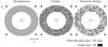 |
Fig. 1 Representation of some 3D homogeneous and clumpy geometries studied in this paper. The star distribution is always localized in the centre of the shell, whereas the dust and the H i content are distributed around. The dust and H i distribution can be “homogeneous” (left), “clumpy” (middle) or “extremely clumpy” (right). In a “clumpy” distribution, the clumps and the interclump medium receive, respectively, high and low densities of dust and HI. In the case of an “extremely clumpy” distribution, all the dust and the H i content are distributed in clumps. |
Other studies have also invoked a higher transmission of Lyα photons than for the UV continuum, to explain observations of some low-redshift LAEs (Scarlata et al. 2009), to understand the overall SED of LAEs at z ~ 4 (Finkelstein et al. 2008, 2009) and to reproduce the Lyα and UV luminosity function of distant galaxies (Dayal et al. 2009; Forero-Romero et al. 2011). Here, we investigate the Neufeld scenario further and examine the physical conditions under which a clumpy ISM could produce a boost of the Lyα line relative to the continuum.
The remainder of this paper is structured as follows. In Sect. 2 we describe our numerical model, presenting the features of the clumpy media and our assumptions. Sections 3 and 4 present our results. The Lyα radiative transfer in homogeneous and clumpy media is presented in Sect. 3, whereas the formation and the features of the emergent Lyα line profiles are described in Sect. 4. Section 5 is dedicated to the discussion of these results with, in particular, an application of our study to the Neufeld scenario. Finally, our main conclusions are summarized in Sect. 6.
2. Method
2.1. 3D radiation transfer code
To study the Lyα line and UV-optical continuum radiation transfer in clumpy geometries, we have used the latest version of the 3D Monte Carlo radiative transfer code MCLyα of Verhamme et al. (2006) and Schaerer et al. (2011). To treat the radiation transfer at wavelengths other than Lyα, we also compute the continuum transfer at other wavelengths assuming scattering and absorption by dust. For the present paper we are interested in three wavelengths, listed in Table 2: the Lyα line (λ = 1215.67 Å), its neighboring UV continuum, and the optical B and V bands.
2.2. 3D geometries, model parameters, and model output
Both for simplicity, and since spherically symmetric outflows with a homogeneous H i shell are able to reproduce a wide variety of observed Lyα line profiles in Lyman break galaxies and LAEs (Verhamme et al. 2008; Schaerer & Verhamme 2008; Dessauges-Zavadsky et al. 2010), the same geometry is used to study how a clumpy ISM structure alters the Lyα line and UV continuum. This clumpy geometry is also chosen since it has been shown to reproduce both the observable continuum properties of starburst galaxies and the Calzetti attenuation law (Gordon et al. 1997; Witt & Gordon 2000; Vijh et al. 2003). Finally, this also allows us to make a detailed investigation into the continuity of the extensive grid of radiation transfer models by Schaerer et al. (2011).
In practice we adopt the following simple shell geometries (see Fig. 1): a static or radially expanding, homogeneous, or clumpy shell of H i and dust surrounding the source emitting both Lyα line and continuum photons. Dust and gas (H i) are assumed to be co-spatial in the shell. We assume a point-like central source.
Six input parameters (top) for and derived parameter (bottom) of the homogeneous and clumpy shell models.
2.2.1. Input parameters
The four physical and the two geometrical input parameters of our models, listed in
Table 1, are the following. The radial expansion
velocity vexp, the Doppler parameter b of
the H i, the mean H i column density
 ,
the mean dust absorption optical depth
,
the mean dust absorption optical depth  ,
the clump volume filling factor FF, and the density contrast
nIC/nC
between the interclump and clumpy medium. Each parcel of the shell (clump or interclump)
exhibits the same radial velocity vexp. The Doppler
parameter
,
the clump volume filling factor FF, and the density contrast
nIC/nC
between the interclump and clumpy medium. Each parcel of the shell (clump or interclump)
exhibits the same radial velocity vexp. The Doppler
parameter  reflects the random (thermal + turbulent) motions of the H i. The clumpy
(inhomogeneous) medium is defined by the volume filling factor FF of clumps, by their
density nC, and by the density contrast
nIC/nC
between clumps and interclumps of lower density nIC. The
mean H i column density
is thus related to the (inter)clump density, FF, and the thickness of the shell
L by
reflects the random (thermal + turbulent) motions of the H i. The clumpy
(inhomogeneous) medium is defined by the volume filling factor FF of clumps, by their
density nC, and by the density contrast
nIC/nC
between clumps and interclumps of lower density nIC. The
mean H i column density
is thus related to the (inter)clump density, FF, and the thickness of the shell
L by  (1)Similarly,
one has
(1)Similarly,
one has 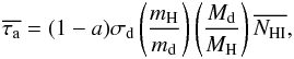 (2)where
a is the dust albedo, σd the total dust
cross section (scattering + absorption), mH the proton mass,
md the dust grain mass, and
(Md/MH) is the dust-to-gas
ratio. In the present paper, the dust optical depth
– the single parameter used to vary the dust content – is derived assuming a dust grain
size of 2 × 10⁻⁶ cm and a mass
md = 3 × 10-17 g. The total dust optical depth
is defined as
(2)where
a is the dust albedo, σd the total dust
cross section (scattering + absorption), mH the proton mass,
md the dust grain mass, and
(Md/MH) is the dust-to-gas
ratio. In the present paper, the dust optical depth
– the single parameter used to vary the dust content – is derived assuming a dust grain
size of 2 × 10⁻⁶ cm and a mass
md = 3 × 10-17 g. The total dust optical depth
is defined as 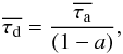 (3)and
the dust particle density is
(3)and
the dust particle density is 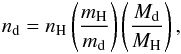 (4)where
nH stands for the clump or interclump density. We adopt
the SMC dust properties (albedo a and phase function
g) listed in Table 2. These properties, together with the clumpy shell
geometry also adopted here, have been shown to reproduce observable continuum properties
of starburst galaxies (Gordon et al. 1997; Witt & Gordon 2000; Vijh et al. 2003). Although detailed model predictions depend to some
extent on the dust properties, the main quantities of interest in this paper – the
Lyα and UV continuum escape fractions, and especially their
relative values – should not strongly depend on the exact dust
properties. We expect that other poorly known properties, such as the geometry and
velocity field, known to affect the transfer of Lyα radiation, are more
important than the detailed dust properties (Laursen et
al. 2009b). For these reasons we have not considered changes in the dust
properties, but focus on the effect of geometry and clumpiness in this paper.
(4)where
nH stands for the clump or interclump density. We adopt
the SMC dust properties (albedo a and phase function
g) listed in Table 2. These properties, together with the clumpy shell
geometry also adopted here, have been shown to reproduce observable continuum properties
of starburst galaxies (Gordon et al. 1997; Witt & Gordon 2000; Vijh et al. 2003). Although detailed model predictions depend to some
extent on the dust properties, the main quantities of interest in this paper – the
Lyα and UV continuum escape fractions, and especially their
relative values – should not strongly depend on the exact dust
properties. We expect that other poorly known properties, such as the geometry and
velocity field, known to affect the transfer of Lyα radiation, are more
important than the detailed dust properties (Laursen et
al. 2009b). For these reasons we have not considered changes in the dust
properties, but focus on the effect of geometry and clumpiness in this paper.
To construct clumpy structures with the desired input parameters in practice, we follow
a similar approach to Witt & Gordon
(2000). We construct a Cartesian grid of N = 1283
cells, within which the shell of thickness L is defined by an inner and
outer radius, Rmin and Rmax.
Assuming a density nC for the high-density regions (clumps),
we then randomly choose a fraction FF of the cells localized in the shell (i.e. cells
localized at a radius R such as
Rmin ≤ R ≤ Rmax),
which receive high density nC. The remaining cells in the
shell are set to low density nIC. The physical cell size (or
equivalently L) is then adjusted to reproduce the desired mean radial
H i column density ,
which is computed by drawing random lines of sight through the shell. Finally the dust
content is varied by changing the dust-to-gas ratio
(Md/MH), thereby yielding
different values of the mean dust absorption optical depth
.
Dust parameters (a and g) taken from Witt & Gordon (2000) and adopted for Lyα line photons, and continuum photons at UV and optical wavelengths (close to the B and V-band).
Range of values of the six input parameters (Cols. 1–6) describing the homogeneous and clumpy shell models, and derived properties (Cols. 7, 8).
In Table 3 we summarize the different values that we explored for the six input parameters describing our models. For the present study we have adopted a filling factor FF = 0.23, as explained below (Sect. 2.2.2). The density contrast nIC/nC was varied from one (homogeneous medium) to nought, reflecting the extreme case of an empty interclump medium. Models were computed for static shells (vexp = 0) and expansion velocities up to vexp = 600 km s-1. Then, a wide range of parameter space was considered, as listed in Table 3.
2.2.2. Characterization of clumpy structures
Given a choice of the clump volume filling factor FF and the thickness of the shell (i.e. Rmax − Rmin), two other interesting quantities describing the inhomogeneous structure can be derived. First, the covering factor CF of the shell corresponding to the fraction of solid angle covered by the clumps as seen from the central source. Models with different covering factors are constructed by varying Rmin.
Another interesting quantity is the mass spectrum of the clumps. As clumps we consider, as does Witt & Gordon (1996, 2000), all cells directly connected with each other by at least one face. We then determine their mass spectrum, which approximately follows a power law ρ(m) ∝ m− α, where m is the clump mass. Adopting FF = 0.23, we obtain a power law ρ(m) ∝ m-2.04 as illustrated in Fig. 2. This mass spectrum is consistent with observations of diffuse interstellar clouds showing a power law with α = 2 (Dickey & Garwood 1989). The value FF = 0.23 in our model is then the most appropriate value if we aim to reproduce the interstellar mass spectrum of nearby galaxies. We illustrate in Fig. 2 the mass spectrum obtained with FF = 0.23 (red curve) in a shell geometry defined with Rmin = 49 and Rmax = 64 cells. The slope of the mass spectrum does not change noticeably, which decreases the covering factor CF (i.e. decreasing Rmin).
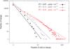 |
Fig. 2 Variation in clump size by adopting different filling factors FF in a shell geometry defined with Rmin = 49 and Rmax = 64 cells. The filling factors used here are FF = 0.07 (circles), FF = 0.13 (diamonds), and FF = 0.23 (triangles). The mass spectrum obtained with FF = 0.23 (ρ(m) ∝ m-2.04) is the most consistent with observations of diffuse interstellar clouds. We thus adopt FF = 0.23 throughout this study. |
We would like to mention that some models with other mass spectra (i.e. other filling factors FF) have been studied, such as ρ(m) ≈ m-2.70 and ρ(m) ≈ m-3.17. However, no notable change is found in any of our results that change only the mass spectrum in clumpy shell structures.
2.2.3. Input spectra
In the region close to Lyα we assume that the spectrum consists of a flat UV continuum (i.e. constant in number of photons per frequency interval) plus the Lyα line, characterized by a Gaussian with an equivalent width EWint(Lyα) and full width at half maximum FWHMint(Lyα). All photons are isotropically emitted from the centre of our shell geometries.
Throughout this work, we adopt FWHMint (Lyα) = 100 km s-1, as a typical value for the intrinsic width of the H recombination lines emitted in the ionized gas, observed in both nearby and distant starburst galaxies. Indeed, based on observations of the velocity dispersion in starburst galaxies, this line width is comparable to the values measured from the velocity dispersion of CO and Hα lines in the starburst galaxy cB58 (Teplitz et al. 2000; Baker et al. 2004), the velocity dispersion measured in several starbursts at z ~ 2 by Erb et al. (2003), and in SMM J2135-0102 at z = 2.32 by Swinbank et al. (2011). Furthermore, different values of EWint(Lyα), specified below if necessary, have been adopted.
2.2.4. Output parameters
For the present paper we are interested in the following quantities predicted by our Monte Carlo simulations: the average Lyα escape fraction fesc(Lyα), the Lyα line profile, and the escape fraction of continuum photons at UV and other wavelengths fesc(λ). From these we also derive the observed Lyα equivalent width EWobs(Lyα), and the colour excess E(B − V). All quantities are computed by spatially integrating all the photons escaping our spherically symmetric shells. They therefore correspond to average properties for our homogeneous and clumpy structures.
In the present study, the Lyα escape fraction is computed from
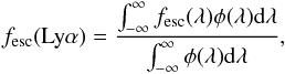 (5)where
fesc(λ) is the monochromatic escape
fraction computed typically for 1000–2000 frequency points around the line centre with a
spacing of 20–10 km s-1, and φ(λ) describes
the input line profile. The predicted Lyα line profile can be computed
a posteriori from our simulations for arbitrary input spectra (line + continuum), as
described in Verhamme et al. (2006). The value of
fesc(Lyα) is slightly dependent on the
FWHM of the input line profile, but independent of the value of
EWint(Lyα).
(5)where
fesc(λ) is the monochromatic escape
fraction computed typically for 1000–2000 frequency points around the line centre with a
spacing of 20–10 km s-1, and φ(λ) describes
the input line profile. The predicted Lyα line profile can be computed
a posteriori from our simulations for arbitrary input spectra (line + continuum), as
described in Verhamme et al. (2006). The value of
fesc(Lyα) is slightly dependent on the
FWHM of the input line profile, but independent of the value of
EWint(Lyα).
The UV continuum escape fraction fesc(UV) is computed
redwards of the Lyα line. Assuming the Calzetti et al. (2000) attenuation law we can compute the corresponding colour
excess as 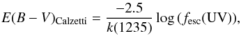 (6)with
k(1235) = 11.4 according to the Calzetti law.
(6)with
k(1235) = 11.4 according to the Calzetti law.
From the escape fraction of radiation at the optical wavelengths listed in Table 2 we can also determine the true colour excess
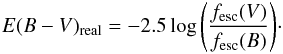 (7)In
practice this is done by calculating the continuum escape fractions at 4350 Å for the
B band and at 5500 Å for the V band (Table 2).
(7)In
practice this is done by calculating the continuum escape fractions at 4350 Å for the
B band and at 5500 Å for the V band (Table 2).
The observed Lyα equivalent width and the intrinsic one (i.e. input
value of the source, before radiation transfer) are related by 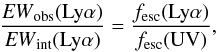 (8)where
EWint(Lyα) is the
intrinsic Lyα equivalent width.
(8)where
EWint(Lyα) is the
intrinsic Lyα equivalent width.
2.2.5. Validation
To test the radiation transfer, we have compared our results to Witt & Gordon (2000), whose dust parameters are adopted in our calculations. We constructed a clumpy shell model using the same discretization and input parameters. The derived mass spectrum is in good agreement with these authors. The resulting continuum escape fractions, shown in Fig. 3, and other results are found to agree very closely with Witt & Gordon (2000), which validates our code.
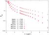 |
Fig. 3 Comparison of the UV-to-optical continuum escape fraction derived from our code with the results of Witt & Gordon (2000). The clumpy shell geometry studied here is built on a Cartesian grid of N = 303 cells and is characterized by the following parameters: FF = 0.15, nIC/nC = 0.01, Rmin = 5, and Rmax = 15. The evolution of the escape fraction at 25 different wavelengths is shown, from λ = 0.1 μm to λ = 30 μm, assuming three different dust optical depths τV in the shell structure (measured in V band): τV = 2, 4.5, and 8. The escape fractions obtained with MCLyα are marked in red, whereas those obtained by Witt & Gordon (2000) are marked in grey. We find very good agreement with Witt & Gordon (2000). |
3. The Lyα and UV continuum radiation transfer in homogeneous and clumpy media
In this section we study the radiative transfer of Lyα and the UV continuum photons in homogeneous and clumpy shell geometries.
3.1. The UV continuum escape fraction
In Figs. 4 and 9, we examine the evolution of the UV escape fraction fesc(UV) in homogeneous and clumpy media. As shown in both figures, fesc(UV) depends on three main parameters:
-
1)
the dust content (
);
-
2)
the clumpiness of the dust distribution, assumed to trace the H i distribution (nIC/nC);
-
3)
the covering factor (CF).
The other parameters describing our shell geometries, the outflows
(vexp), the H i column density
(),
and the temperature of the matter (b) do not show any effect on the UV
escape fraction, as expected.
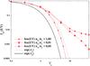 |
Fig. 4 Evolution of the UV escape fraction fesc(UV) as a
function of the dust optical depth ( |

Figure 4 illustrates the effects produced by both
the dust content (i.e. )
and the clumpiness of the dust distribution (i.e.
nIC/nC) on
fesc(UV). We adopt here three media with the following
conditions: FF = 0.23, CF = 0.997, and
nIC/nC = 1.0, 0.01, 0.
Qualitatively, we can summarize the effects produced by both
and nIC/nC on
fesc(UV) in the following way:
-
:
in homogeneous and clumpy media, an increase in the dustoptical depth
always produces adecrease in the UV escape fraction.
-
nIC/nC: a decrease in nIC/nC from 1 to 0 (i.e. from a homogeneous to an extremely clumpy dust distribution) always increases the UV escape fraction. A clumpy dust distribution indeed produces higher UV escape fractions than does an equivalent homogeneous distribution of equal dust content (i.e. equal
).
Clumpy media are thus more transparent to UV continuum radiation, as previously shown by Boisse (1990), Hobson & Scheuer (1993), Witt & Gordon (1996, 2000). That the dust content concentrates in clumps and that the interclump medium becomes more optically thin allow UV photons to escape any clumpy media in two different ways (Witt & Gordon 1996): first, as in homogeneous dusty media, UV photons have to scatter against few dust grains before escaping clumpy media (dust localized in clumps or in between clumps). But, in clumpy media, UV photons take advantage of the weak opacity of the inter-clump medium, which allows them to escape clumpy media more easily than any homogeneous dusty geometry. Second, continuum photons can also directly escape clumpy media if several free spaces appear between clumps. However, that can only be possible in extremely clumpy media (nIC/nC ≈ 0). In this case, continuum photons are not affected by the weak dust content localized between clumps and can directly escape clumpy media getting through the holes that appear between clumps.
The covering factor CF is thus an important parameter controlling the UV escape fraction in clumpy media. Figure 9 shows this dependence in the particular case of extremely clumpy shell geometries (nIC/nC = 0). As expected, the UV escape fraction fesc(UV) decreases when the covering factor increases to unity (i.e. all lines-of-sight are covered by one or more clumps from the photon source when CF = 1). Furthermore, in the particular case of extremely clumpy shell geometries (nIC/nC = 0), we can also notice that the covering factor CF provides a general lower limit for fesc(UV). As shown in Figs. 4 and 9, the UV escape fraction always converges on an asymptote fesc(UV) = 1−CF, corresponding to the direct escape fraction.
Besides this qualitative approach to the dependence of
fesc(UV) to ,
nIC/nC and CF, Fig. 4 illustrates other quantitative results: in homogeneous
geometries the UV escape fraction decreases very rapidly with the dust optical depth
.
If we define fesc(UV) =
e−τeff, the effective optical depth
τeff is equal to
in the absence of scattering. With scattering the effective absorption increases, and one
has  .
In clumpy media the situation is different because photons can escape more easily, hence
.
In clumpy media the situation is different because photons can escape more easily, hence
 .
.
The escape fraction of the optical continuum photons evolves in the same way as for the
UV photons in homogeneous and clumpy media. Combining the escape fraction of both the
B and the V-band in the same media as those studied in
Fig. 4, we illustrate in Fig. 17 the evolution of the derived colour excess
E(B − V). This figure can be used to
translate the dust optical depth
of Fig. 4 in terms of colour excess
E(B − V).
3.2. The Lyα radiative transfer in homogeneous and clumpy media: two regimes appear
Besides the three main parameters that control the radiative transfer of the UV continuum
photons (i.e. ,
nIC/nC and CF), three other
parameters also determine the radiative transfer of the resonant scattered
Lyα photons, namely vexp,
,
and b. We now discuss the influence of these parameters on the UV
continuum and on Lyα. For simplicity we assume a constant value of
b in all cells (clump or interclump). Overall we find that we can
identify two regimes where the Lyα propagation is quantitatively
different, which we now explain. The separation between the regimes is discussed after
that (Sect. 3.3).
3.2.1. The low-contrast regime: homogeneous and weakly clumpy media
Propagation of Lyα photons in the low-contrast regime: we show in Fig. 5 the typical way Lyα photons propagate in the low-contrast regime. We deduce this propagation from our numerical simulations by studying the number and the location of each interaction between the Lyα photons and the HI atoms in clumpy media. In this regime, we notice that the Lyα radiative transfer is characterized by a (pseudo-)random walk in the medium, both in and between clumps.
Lyα escape fraction
fesc(Lyα): Fig. 6 shows the dependence of
fesc(Lyα) on the dust content
()
of the medium, for different values of clumpiness
(nIC/nC). The low-contrast
regime includes all curves of this figure, except the particular case
nIC/nC = 0.00, which belongs
to the high-contrast regime. The quantity
can be related to the colour excess through Fig. 17.
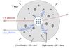 |
Fig. 5 Schematic representation of how UV continuum (red) and Lyα photons (blue) propogate in the low-contrast regime. The medium illustrated here is composed of high-density clumps (containing H i + dust), distributed in an interclump medium of low density (HI+dust). In the low-contrast regime, the H i content in and between clumps are relatively high, which renders both regions optically thick for the Lyα photons. In this way, the Lyα photons can only escape the medium after undergoing multiple resonant scattering against H i atoms, increasing their probability being absorbed by the dust. The UV photons are not affected by the presence of H i atoms and propagate directly through the medium. |
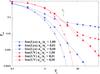 |
Fig. 6 Evolution of the Lyα (blue lines) and UV continuum (red) escape
fraction as a function of the dust optical depth
( |
Qualitatively, we see that fesc(Lyα)
always decreases with increasing ,
as expected. The same is true for increasing
nIC/nC. However, we see that
for a given value of ,
increasing nIC/nC results in a
faster decrease of fesc(Lyα) than
fesc(UV), the reason being the highly increased path
length of Lyα photons due to resonant scattering. Thus, in the
low-contrast regime, Lyα radiation is more vulnerable to dust than UV
continuum radiation.
A change in the covering factor CF also has a noticeable effect on fesc(Lyα) in the low-contrast regime (CF measuring the proportion of holes that appear between clumps). As the clumps cover an increasing fraction of the sky, it indeed becomes increasingly difficult for the photons to escape, and when CF ≈ 1, fesc(Lyα) drops drastically.
Finally, the effect of a change in vexp and
on fesc(Lyα) is shown in Fig. 7. We notice that
fesc(Lyα) always increases with
increasing vexp, as well as with
decreasing. Since the effect of the expansion velocity is to shift the
Lyα photons away from the line centre, they undergo progressively
fewer scattering as vexp increases. In fact, for an
intrinsic Lyα line width of
FWHMint(Lyα) (this value is 100
km s-1 in Fig. 7), a galactic outflow
showing a velocity
vexp ≳ 2 × FWHMint(Lyα)
is enough to allow Lyα photons to escape as easily as UV continuum
photons. As expected, an increase in
always leads to a decrease in fesc(Lyα),
since more neutral hydrogen implies more scatterings, hence an increased total path
length before escape, resulting in an increased probability of being absorbed.
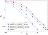 |
Fig. 7 Evolution of the Lyα escape fraction
fesc(Lyα) as a function of dust
optical depth |
Quantitatively, both Figs. 6 and 7 allow us to generalize the fact that, in the low
contrast regime, we always obtain
 (9)The
strict equality fesc(Lyα) =
fesc(UV) is only met when Lyα photons are
able to avoid scatterings altogether, i.e. for sufficiently high expansion velocity or
for very low H i column density.
(9)The
strict equality fesc(Lyα) =
fesc(UV) is only met when Lyα photons are
able to avoid scatterings altogether, i.e. for sufficiently high expansion velocity or
for very low H i column density.
Lyαequivalent width
EW(Lyα):
combining the definition of the Lyα equivalent width (Eqs. (8)) and
(9), we always have 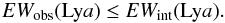 (10)In
the low-contrast regime, the EWobs(Lya) is
thus always lower or equal to the intrinsic one
EWint(Lya). In other words, the
Lyα equivalent width cannot be “boosted” by clumping in this regime.
(10)In
the low-contrast regime, the EWobs(Lya) is
thus always lower or equal to the intrinsic one
EWint(Lya). In other words, the
Lyα equivalent width cannot be “boosted” by clumping in this regime.
3.2.2. The high-contrast regime: extremely clumpy shell geometries
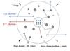 |
Fig. 8 Schematic representation of the way the UV continuum (red) and the Lyα (blue) photons propogate in the high-contrast regime. The medium illustrated here is composed of high-density clumps (H i + dust), distributed in an empty interclump medium. A fraction of the Lyα photons scatter on the H i atom comprising the surface of the clumps. The rest of the Lyα photons, as well as the UV continuum photons, pierce the clumps where they may be absorbed by dust. |
The high-contrast regime of the Lyα radiative transfer is defined by clumpy media showing a very low ratio nIC/nC, i.e. a high density contrast at least nIC/nC ≲ 1.5 × 10⁻⁴ for the input parameters considered throughout this study (see Sect. 3.3). To describe the main effects and peculiarities of this regime we restrict ourselves here to the most extreme case with nIC/nC = 0.
Propagation of Lyα photons in the high-contrast regime: the way Lyα photons propagate now differs qualitatively from the radiative transfer in the low-contrast regime. The details of the way we deduce the propagation of Lyα photons in the high-contrast regime are given in Sect. 4, where we study the Lyα line shape. We sketch in Fig. 8 the propagation of Lyα photons in the high-contrast regime. The H i content distributed between clumps is now weak enough that scattering between clumps can be neglected, and for a fraction of the Lyα photons, the radiative transfer is characterized by rebounces on the clumps, as originally suggested by Neufeld (1991). The remaining Lyα photons propagate in the same way as UV photons, which is penetrating the clumps, being exposed to the dust, or escaping the medium freely (if CF < 1).
Lyα escape fraction
fesc(Lyα): Fig. 6 shows the evolution of
fesc(Lyα) as a function of the dust
content (i.e. )
in the high-contrast regime
(nIC/nC = 0). Again, the
quantity
can be related to the colour excess through Fig. 17. From Fig. 6 it is evident that
fesc(Lyα) always decreases as
increases. However, the decrease is slower than for
fesc(UV), allowing the curve of
fesc(Lyα) to cross that of
fesc(UV) at a certain optical depth
τc (τc ≈ 3.8 in Fig. 6). This is not possible in the low-contrast regime,
and it is this quantitative difference that defines the threshold between the low- and
the high-contrast regimes.
Figure 9 illustrates the effect of a change in the covering factor CF on fesc(Lyα) in the high-contrast regime. Again, we see that both fesc(Lyα) and fesc(UV) always decrease with increasing CF. However, whereas fesc(UV) approaches the value 1 − CF asymptotically (corresponding to all clumps being fully opaque to the UV so that escape is possible only through direct escape), fesc(Lyα) maintains a higher value. Furthermore, we can notice from Fig. 9 that the value of the critical optical depth τc (where fesc(Lyα) crosses fesc(UV)) strongly decreases as CF decreases.
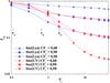 |
Fig. 9 Lyα (blue lines) and UV (red lines) escape fraction as a
function of the dust optical depth |
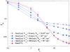 |
Fig. 10 Lyα (blue lines) and UV (red line) escape fractions as a
function of the dust optical depth |
The effect of a change in vexp and
on fesc(Lyα) is shown in Fig. 10. We can see that these effects are different and
more complex than those of the low-contrast regime. More precisely, two different
domains appear in the high-contrast regime, below and above the critical optical depth
τc (where
fesc(Lyα) crosses
fesc(UV)). Below τc, we notice
that fesc(Lyα) increases with increasing
vexp, as well as with
decreasing. This behaviour is the same as in the low-contrast regime. But above
τc, the opposite effect is observed, where an increase of
fesc(Lyα) results from a decrease of
vexp and an increase of
.
These distinct behaviors can be understood as follows (see Fig. 8):
-
 : in this
domain, Lyα photons are more vulnerable to dust than UV photons.
The dust content being relatively low, each clump is optically thin for UV
radiation, which allows UV photons to escape directly from the medium, thereby
getting through the clumps. However, Lyα photons have to scatter
off of the surface of a high number of clumps before escaping (Fig. 8), which
increases the probability of being absorbed by the dust. An increase in
vexp increases the Lyα escape
fraction fesc(Lyα). Indeed, by
increasing the expansion velocity vexp, all Lyα
photons are Doppler-shifted out of resonance, forcing them to pierce the clumps
and thus to escape the medium as easily as UV photons. For the same reason, a
decrease in
increases fesc(Lyα) because it reases
the H i density in clumps. It therefore renders clumps more transparent
to Lyα photons.
: in this
domain, Lyα photons are more vulnerable to dust than UV photons.
The dust content being relatively low, each clump is optically thin for UV
radiation, which allows UV photons to escape directly from the medium, thereby
getting through the clumps. However, Lyα photons have to scatter
off of the surface of a high number of clumps before escaping (Fig. 8), which
increases the probability of being absorbed by the dust. An increase in
vexp increases the Lyα escape
fraction fesc(Lyα). Indeed, by
increasing the expansion velocity vexp, all Lyα
photons are Doppler-shifted out of resonance, forcing them to pierce the clumps
and thus to escape the medium as easily as UV photons. For the same reason, a
decrease in
increases fesc(Lyα) because it reases
the H i density in clumps. It therefore renders clumps more transparent
to Lyα photons. -
 : in this
domain, Lyα photons are less affected by the dust than UV
photons. Indeed, while UV photons are now strongly absorbed by the high dust
content embedded in clumps, Lyα photons can avoid interaction
with dust scattering off of the surfaces of clumps. An increase in
vexp results in a decrease in
fesc(Lyα). By increasing the
expansion velocity, all Lyα photons are Doppler-shifted out of
resonance, forcing them to pierce the clumps, where they are strongly absorbed by
the dust-like UV photons. For the same reason,
fesc(Lyα) now increases with
increasing
because increasing the H i content of the clumps increases the
probability of Lyα photons scattering off the clumps, with the
journey confined to the dust-free interclump medium.
: in this
domain, Lyα photons are less affected by the dust than UV
photons. Indeed, while UV photons are now strongly absorbed by the high dust
content embedded in clumps, Lyα photons can avoid interaction
with dust scattering off of the surfaces of clumps. An increase in
vexp results in a decrease in
fesc(Lyα). By increasing the
expansion velocity, all Lyα photons are Doppler-shifted out of
resonance, forcing them to pierce the clumps, where they are strongly absorbed by
the dust-like UV photons. For the same reason,
fesc(Lyα) now increases with
increasing
because increasing the H i content of the clumps increases the
probability of Lyα photons scattering off the clumps, with the
journey confined to the dust-free interclump medium.
Finally, as in the low-contrast regime, we notice that a velocity vexp ≳ 2 × FWHMint(Lyα) is enough to prevent any scattering on the clumps. In this case, Lyα photons escape the medium in the same way as UV photons.
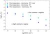 |
Fig. 11 Evolution of the critical ratio nIC/nC separating the low-contrast regime from the high-contrast regime of the Lyα radiative transfer in clumpy shell geometries. For highest ratio nIC/nC, all clumpy media belong to the low-contrast regime, whereas for lower nIC/nC the high-contrast regime is observed. Three curves are represented in this figure corresponding to the three different physical conditions applied to our clumpy media (see text). |
Lyα equivalent width EW(Lya):
qualitatively, Figs. 6, 9, and 10 reveal that in the
high-contrast regime fesc(Lyα) can be both
higher or lower than fesc(UV), depending on the actual value
of .
From the definition of τc (i.e. the value of
where the curves of fesc(Lyα) and
fesc(UV) cross each other), we have  (11)and
 (12)where
we note that τc is mainly a function of CF.
(12)where
we note that τc is mainly a function of CF.
Combining the definition of the Lyα equivalent width (Eq. (8)) with both Eqs. (11) and (12), we obtain
 (13)and
 (14)That
fesc(Lyα) can exceed
fesc(UV) thus allows for an enhancement (“boost”) of the
equivalent width of the Lyα line. However, as summarized in Sect. 5.2,
such an enhancement can only occur under strict physical conditions, concerning the
kinematics (i.e. an expansion velocity
vexp ≲ 2 × FWHMint(Lyα)),
the clumpiness and the dust content of the clumpy ISM.
(14)That
fesc(Lyα) can exceed
fesc(UV) thus allows for an enhancement (“boost”) of the
equivalent width of the Lyα line. However, as summarized in Sect. 5.2,
such an enhancement can only occur under strict physical conditions, concerning the
kinematics (i.e. an expansion velocity
vexp ≲ 2 × FWHMint(Lyα)),
the clumpiness and the dust content of the clumpy ISM.
3.3. The critical ratio nIC/nC separating the two regimes of the Lyα radiative transfer
We can quantify the distinction between the two regimes of the Lyα
radiative transfer by the low-to-high density ratio
nIC/nC.
Figure 11 illustrates this limit
nIC/nC as a function of the
average H i column density
in our clumpy media. This limit is defined in the following way. Above the curves shown in
Fig. 11, it is impossible to obtain fesc(Lyα)
>fesc(UV) in models with the
physical parameters listed in Table 3. These media belong to the low-contrast regime.
Conversely, the area localized below the curves corresponds to the high-contrast regime,
where it is possible to observe the inequality
fesc(Lyα)
>fesc(UV).
All points shown in Fig. 11 have been obtained by
studying a clumpy medium defined with FF = 0.23, CF = 0.997,
vexp = 0 km s-1,
= 25, and b = 40 km s-1. All media built with different
parameters show a critical ratio
nIC/nC (at
the limit between the low- and the high-contrast regimes) that is lower than the one shown
in Fig. 11. Each curve shown in this figure
corresponds to three different physical conditions applied in our clumpy media. The star
dots are obtained by assuming a unique turbulent velocity b = 40
km s-1 in and between clumps, and an inter-clump medium composed of both
H i atoms and dust grains. The circle dots are obtained assuming the same
turbulent velocity (b) but a dust-free interclump medium. Finally, the
squares are obtained by applying two different temperatures in clumps and between clumps
(b = 40 km s-1 in clumps and
T = 106 K between clumps) and assuming an interclump medium
only composed of H i atoms. This case is discussed in Sect. 3.4.
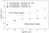 |
Fig. 12 Same as in Fig. 11, but showing the evolution
of the H i column density between clumps
NHI,IC (= (1 – FF)
× nICL, with L as the physical size of the shell), as
a function of the total |
From the single-temperature case, we can already mention four main results concerning the border separating the two regimes of the Lyα radiative transfer:
The critical ratio
nIC/nC
separating both regimes is very low: studying a wide range of H i
column density
[1017, 1022] cm-2, we notice that the limit separating
both regimes is reached for very weak ratios
nIC/nC ([1.5 × 10⁻⁴,
1.3 × 10⁻⁶]). That suggests that the high-contrast regime can only be found
in galaxies that show the most extremely clumpy ISMs (composed only of cold clouds of
neutral hydrogen gas embedded in an extremely ionized interclump medium). The critical
ratio has to decrease with increasing
to maintain a low enough column density between the clumps.
The interclump medium can be optically thick for Lyα photons on the border separating the two regimes: in Fig. 12 we show the limit of Fig. 11, but translated in terms of HI column density between clumps NHI,IC = (1−FF) × nICL. While the interclump medium is optically thick for Lyα photons at line centre above NHI,IC = 6 × 1013 cm-2 (assuming b = 40 km s-1 between clumps)1, we can clearly see that the high-contrast regime can extend to somewhat higher interclump column densities, into the optically thick regime. Nevertheless, this is only possible if the temperatures in and between clumps are the same. If the temperatures in and between the clumps differ, the interclump medium has to be optically thin to observe the high-contrast regime (see Sect. 3.4).
The limit nIC/nC separating both regimes is not affected by the presence of dust between clumps: the critical ratio nIC/nC represented by both the star and the circle dots in Fig. 11 are the same. Thus, the presence of dust between clumps has no effect on the limit separating both regimes of the Lyα radiative transfer.
3.4. The effects of inhomogeneous temperature on the Lyα radiative transfer
If we want to render the physics of our clumpy media more realistic, we must assume different temperatures inside and between the clumps. There is ample evidence for such a multi-phase ISM. For example, for the stability of the clumps a pressure equilibrium should intervene between the two phases of our clumpy media, implying higher temperature in the interclump medium. Also, it is well known that different regions coexist in the real ISM of any galaxies (McKee & Ostriker 1977). In particular, we can distinguish the warm neutral atomic medium (WNM, where H i atoms are present in the atomic form) to the hot ionized medium (HIM, where the great majority of the H i atoms are ionized). To explore these effects in a simplified manner, we made calculations assuming a temperature of T = 106 K in the interclump medium (like those measured in the HIM), but a lower temperature in all clumps (b = 40 km s-1, by analogy to the WNM). We then examine the effects on the Lyα radiative transfer and on the ratio nIC/nC separating the two regimes identified above.
Qualitatively, the Lyα radiative transfer properties behave in a similar fashion for different interclump temperatures. However, as shown in Fig. 11, the ratio nIC/nC separating both regimes is found to be lower than for the case of constant temperature. In other words, the high-contrast regime is more limited when the temperature in the interclump medium is higher than those in clumps. The reason for this is the following: on one hand, the optical depth in the interclump medium decreases (with T−1/2), thus simulating a medium with even lower density, i.e. higher contrast. On the other hand, the temperature increase leads to a larger frequency redistribution of the scattered Lyα photons, which eases their escape due to higher frequency shifts. This effect dominates the former, thus rendering the clumps more transparent to Lyα radiation, where they are strongly absorbed by the dust. This explains why even higher density contrasts are needed to achieve significant Lyα “rebounce” on the clumps, if the interclump medium is hotter than the clumps.
In terms of interclump column densities, the limit between the regimes is shown in Fig. 12. In contrast to the case of uniform “cold” temperatures, the limit is now found at quite low column densities of the interclump medium, corresponding to an optically thin regime. Indeed, such low column densities are needed if one wants to avoid significant scattering of Lyα with the corresponding high-frequency shifts in a hot interclump medium.
4. Lyα line profiles formation in homogeneous and clumpy shells
In this section we give an overview of the different emergent Lyα line profiles produced in the expanding homogeneous and clumpy shell geometries of our model.
4.1. Lyα line profiles from dust free homogeneous and clumpy shell geometries
First, we consider the case of a dust-free ISM and examine how the Lyα profiles are modified by a clumpy ISM structure. The line profiles shown in this section are obtained assuming an intrinsic Lyα line characterized by EWint(Lyα) = 80 Å and FWHMint = 100 km s-1.
We know that in dust-free cases the total Lyα flux is preserved, and since the continuum is not attenuated (due to the absence of absorption), the Lyα equivalent width is thus preserved; in other words, the observed EW is identical to the intrinsic one. This obviously holds both for homogeneous and clumpy structures. The only effect of clumps is to modify the exact frequency redistribution of photons, i.e. the shape of the emergent Lyα line profile. However, as we will see, the changes to the line profile are only relatively small, when the covering factor of the clumps is large.
We first examine the Lyα line profiles for dust-free homogeneous and
clumpy structures with low density contrast (i.e. clumpy structures showing an optically
thick interclump medium for Lyα photons). In Fig. 13 we study such structures built with the following parameters:
nIC/nC =
1.00, 0.01,  cm-2,
b = 40 km s-1, and vexp = 0,
100, 300, 400 km s-1. It clearly appears that the Lyα line
profiles emerging from dust-free, weakly clumpy shell geometries do not show any
noticeable difference compared to homogeneous structures with the same/corresponding
properties.
cm-2,
b = 40 km s-1, and vexp = 0,
100, 300, 400 km s-1. It clearly appears that the Lyα line
profiles emerging from dust-free, weakly clumpy shell geometries do not show any
noticeable difference compared to homogeneous structures with the same/corresponding
properties.
In homogeneous and weakly clumpy media, the mechanisms of formation of the line profiles,
as well as their dependence on the parameters vexp,
,
and b, are identical to those explained in detail in Verhamme et al. (2006) for homogeneous shell
structures. In other words, in the dust-free case, weakly clumpy media do not
significantly differ from the homogeneous ones in terms of line profiles.
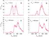 |
Fig. 13 Comparison between the Lyα line profiles emerging dust free
homogeneous shell (dotted blue lines), weakly clumpy shell (dashed magenta lines)
and extremely clumpy shells (thick red lines) under different expansion velocities
vexp. All homogeneous and clumpy shells have for
common parameters: |
Turning now to clumpy media with high density contrasts (i.e. clumpy structures showing an optically thin interclump medium for Lyα photons, such as nIC/nC = 0,00), we find again very similar line profiles as in the homogeneous case, as also shown in Fig. 13. Compared with the line profiles observed from static weakly clumpy and homogeneous media we now see a central peak at line centre (vobs ≈ 0 km s-1). The formation of this central peak is indeed made possible when the interclump medium is optically thin for Lyα photons. These photons can then propagate in two different ways in the interclump medium: either by escaping through the holes that appear between clumps or scattering off of the surface of clumps. Both features preserve the intrinsic frequency of the Lyα photons, which allows formation of the central peak seen at centre of the Lyα line (vobs ≈ 0 km s-1). The covering factor mostly governs the importance of the central emission, as shown in Fig. 14 for a static shell. As expected, the central emission increases with decreasing the covering factor.
Besides this, the predicted Lyα line profiles in dust-free clumpy shell
geometries behave in the same way as already shown for homogeneous shells by Verhamme et al. (2006), where the main parameters
determining the Lyα profile are the expansion velocity
vexp, the mean HI column density
,
and the Doppler parameter b.
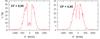 |
Fig. 14 Effect of the covering factor CF on the Lyα line profiles in
extremely clumpy shell geometries. We study here a static, extremely clumpy shell
geometry defined with the following parameters: FF = 0.23,
nIC/nC = 0.00,
|
4.2. Lyα line profiles from dusty homogeneous and clumpy shell geometries
We now examine the main effects produced by dust on the Lyα line
profiles emerging from clumpy shell geometries. In Fig. 15 we illustrate the evolution of the line profiles predicted for static
homogeneous and clumpy shell geometries as a function of the dust optical depth
.
The top line shows the homogeneous case, the middle the low density contrast, and the
bottom line the clumpy medium with a high density contrast. We first examine the
homogeneous and low density contrast cases
(nIC/nC =
1.00 and 0.01 respectively). Increasing
from 0 to 1, the Lyα line still appears in emission in both cases. But, a
clear decrease in both the width and the intensity of each peak is noticed. For
= 3, more than 99.8% and 98% of the Lyα photons are absorbed by the dust,
respectively, in the homogeneous and the weakly clumpy medium. Therefore, an absorption
profile emerges from the homogeneous medium, while faint emission line is predicted from
the weakly clumpy medium. Higher dust optical depths
are needed to obtain absorption line profiles from weakly clumpy media, typically
 in the
case of nIC/nC = 0.01.
in the
case of nIC/nC = 0.01.
For extremely clumpy shell geometries
(nIC/nC = 0.00, Fig. 15), the evolution of the Lyα line
profile is different. Increasing
from 0 to 1, we notice a clear decrease in the width of both lateral peaks, as well as an
increase in the relative intensity of the central peak. The photons composing the central
peak indeed interact very weakly with the dust, which explains why this peak becomes the
dominant one in the line profile as
increases. When
is further increased from 1 to 3, both lateral peaks are destroyed by dust. The central
peak thus becomes the only peak composing the line profile above
 . It is
interesting to note that we cannot obtain absorption line profiles in extremely clumpy
media (nIC/nC = 0.00). Indeed, as
the Lyα photons composing the central peak interact very weakly with
dust, they are always able to escape the medium for any dust optical depth
,
thus giving rise to an emission line. Comparing the relative escape of the
Lyα and UV continuum photons, we note that the only case in Fig. 15 where the Lyα equivalent width is
(slightly) enhanced is found in the bottom right-hand panel. Indeed, in this case
is close to the critical dust optical depth τc ≈ 3 for this
example of extremely clumpy medium, where we expect such an enhancement (cf. Sect. 3.2.2).
. It is
interesting to note that we cannot obtain absorption line profiles in extremely clumpy
media (nIC/nC = 0.00). Indeed, as
the Lyα photons composing the central peak interact very weakly with
dust, they are always able to escape the medium for any dust optical depth
,
thus giving rise to an emission line. Comparing the relative escape of the
Lyα and UV continuum photons, we note that the only case in Fig. 15 where the Lyα equivalent width is
(slightly) enhanced is found in the bottom right-hand panel. Indeed, in this case
is close to the critical dust optical depth τc ≈ 3 for this
example of extremely clumpy medium, where we expect such an enhancement (cf. Sect. 3.2.2).
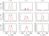 |
Fig. 15 Effects of the dust optical depth |
We now turn to a case with outflows in Fig. 16. In
this figure, we adopt otherwise identical parameters to those shown in Fig. 15. Increasing
in any media (homogeneous or clumpy), we first notice a quick decrease in the intensity of
both the dominant red peak (the one located close to the line centre and the one shifted
at vobs = 2 × vexp) and the small
blue bump. This is due to the higher number of scatterings these photons undergo, which
increases their destruction probability, as already discussed by Verhamme et al. (2006). For the highest dust content
(
= 3), the Lyα line escaping homogeneous and clumpy media exhibits an
asymmetric profile, but the dominant peak is found at line centre
(vobs = 0). Finally, as in the static case, we notice that
the intensity of the line increases as the clumpiness of the medium increases. In none of
the cases shown here we find a “boost” of the Lyα equivalent width, since
the velocity is too high.
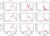 |
Fig. 16 Same as Fig. 15 but for an expanding shell with vexp = 300 km s-1. No boost of Lyα with respect to the continuum is found in any of these models, since the expansion velocity is too high. Discussion in the text. |
5. Discussion
5.1. Effects of a clumpy ISM on the radiation attenuation
Given the evolution of the Lyα and continuum escape fraction in homogeneous and clumpy systems (Sect. 3), it is clear that a clumpy medium always produces higher Lyα and continuum escape fraction compared with an equivalent homogeneous medium of equal dust and hydrogen mass. This main result was demonstrated by several previous studies focussed on the transfer of the continuum radiation in clumpy media (Boisse 1990; Hobson & Scheuer 1993; Witt & Gordon 1996, 2000; Varosi & Dwek 1999), but also from other studies focussed on the Lyα line (Neufeld 1991; Hansen & Oh 2006).
The attenuation of the radiation in a galaxy thus strongly depends on both the dust
content and the dust distribution around the radiation sources. As an illustration, we
show in Fig. 17 the dependence of the colour excess
E(B − V) on both the dust content
()
and the clumpiness of the dust distribution in the shell geometries studied throughout
this paper. In this figure we compare two different definitions of the colour excess:
E(B − V)real, which
corresponds to the exact colour excess because estimated from the original definition of
the colour excess (from the V and B bands), and
E(B − V)Calzetti, which is
estimated from both the Calzetti attenuation law (Calzetti
et al. 2000) and the UV escape fraction (see Eqs. (6) and (7)). In
practice, the Calzetti attenuation law is usually used to estimate the dust attenuation in
starburst galaxies. It is then
E(B − V)Calzetti, which
would be measured by an observer. Figure 17 then
allows us to see to what extent the colour excess
E(B − V)Calzetti, from the
Calzetti law, deviates from the real colour excess
E(B − V)real as a function
of
and the clumpiness of the dust distribution.
In a general way, we can notice that the clumpiness of the dust distribution strongly affects both the colour excess E(B − V)real and E(B − V)Calzeti (Witt & Gordon 2000). The colour excess decreases as the dust distribution is clumpy and as the dust optical depth decreases in media. Comparing now both definitions of E(B − V)Calzetti and E(B − V)real, we can notice that E(B − V)Calzetti does not reproduce the real evolution of the colour excess E(B − V)real very well. This deviation between both definitions is explained by a clear evolution of the attenuation law (which measures, at each wavelength, the reduction in the stellar flux from a dusty ISM) as the dust distribution and the dust content change in media. As mentioned in Witt & Gordon (2000), this divergence shows that the use of the same and unique attenuation law in the analysis of a large sample of galaxies (which show different dust geometries and dust content) can become a source of error in the dust attenuation correction for individual galaxies.
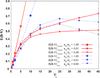 |
Fig. 17 Evolution of the colour excess
E(B − V) as a function of
|
5.2. High Lyα EWs and the Neufeld model
5.2.1. Physical conditions needed in the ISM
According to our study of the Lyα transfer in clumpy media, there exists a regime in which the Neufeld scenario works. This regime corresponds to the high-contrast regime, as explained in detail in Sect. 3.2.2. It is only found in the most extremely clumpy shell geometries of our model, which is composed of clouds of H i and dust embedded in an interclump medium close enough to be optically thin for Lyα photons. However, even in this configuration, the Neufeld model only works when the following five main conditions concerning the clumpiness, the kinematic, the dust content, and the spatial distribution of the clumps around the stars are fulfilled.
The galaxy outflow has to be relatively slow:
assuming an intrinsic Lyα line width
FWHMint(Lya), a galactic outflow with an expansion
velocity vexp ≲ 2 × FWHMint(Lya)
km s-1 is needed to be able to enhance
EW(Lyα) under the Neufeld scenario. In starburst
galaxies, the width of the intrinsic Lyα line is lower than 100
km s-1 (Teplitz et al. 2000; Baker et al. 2004; Erb
et al. 2003; McLinden et al. 2011),
which implies an expansion velocity vexp lower than 200
km s-1 in the ISM. We illustrate this limit in Fig. 18. This figure shows the evolution of the ratio
fesc(Lyα)/fesc(UV)
as a function of the dust content (measured here in terms of colour excess
E(B − V)Calzetti) in
extremely clumpy shell geometries. We here adopt b = 12.8
km s-1,  ,
2 × 1020 cm-2, and Vexp = 0, 100,
200 km s-1, which are typical of values obtained in the analysis of
high-z Lyα line profiles (Verhamme et al. 2008). Finally, we mention that the curves shown in
this figure illustrate the highest enhancements of
EW(Lyα) we can obtain when adopting such physical
conditions in a clumpy medium: they reach a factor 3–4. Adopting
FWHM(Lya)int = 100 km s-1 in
Fig. 18 we notice that no significant enhancement
of EW(Lyα) is obtained for
vexp ≳ 200 km s-1. Above such an expansion
velocity, all Lyα photons are Doppler-shifted out of resonance,
preventing them from scattering off of the surface of clumps and from escaping clumpy
ISMs more easily than UV continuum photons.
,
2 × 1020 cm-2, and Vexp = 0, 100,
200 km s-1, which are typical of values obtained in the analysis of
high-z Lyα line profiles (Verhamme et al. 2008). Finally, we mention that the curves shown in
this figure illustrate the highest enhancements of
EW(Lyα) we can obtain when adopting such physical
conditions in a clumpy medium: they reach a factor 3–4. Adopting
FWHM(Lya)int = 100 km s-1 in
Fig. 18 we notice that no significant enhancement
of EW(Lyα) is obtained for
vexp ≳ 200 km s-1. Above such an expansion
velocity, all Lyα photons are Doppler-shifted out of resonance,
preventing them from scattering off of the surface of clumps and from escaping clumpy
ISMs more easily than UV continuum photons.
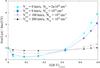 |
Fig. 18 Evolution of the ratio
fesc(Lyα)/fesc(UV)
(i.e. EWobs
(Lya)/EWint(Lya)) as a function of
the colour excess
E(B − V)Calzetti
in four extremely clumpy media. We apply some realistic physical conditions of
LAEs to each media:
nIC/nC = 0.00, FF = 0.23,
CF = 0.997 (Rmin = 49 and
Rmax = 64 cells), b = 12.85
km s-1 (i.e. T = 104 K in clumps),
|
The galaxy outflow has to be relatively uniform (constant velocity): Lyα photons can scatter on the surface of clumps (Fig. 8) under the condition that each clumps move weakly each other. Should the opposite occur (that is, assuming a random component vrandom in the velocity of each clump), a strong Doppler shift can occur between clumps, which prevents Lyα photons from scattering against clumps any more. Finally, such an effect strongly decreases the Lyα escape fraction fesc(Lyα) in a clumpy ISM. In Fig. 19, we illustrate how the enhancements of EW(Lyα) shown in Fig. 18 are affected by a nonuniform outflow. In this figure, we assume a radial and random velocity vclump for each clump, such that vclump = vexp + vrandom, where vrandom = rvmax with r ∈ [−1,1] a random number. We notice a clear decrease in the ratio fesc(Lyα)/fesc(UV) as vrandom increases.
The H I content between
clumps must be extremely small: the Neufeld model was originally developed by
assuming an interclump region that is poor enough in H i atoms that it is
completely transparent to Lyα photons. In our simulations, we have
identified the H i content in the interclump medium to allow the Neufeld
scenario to work. There is indeed a certain H i limit above which
Lyα photons cannot freely propagate between clumps, preventing them
from escaping the medium more easily than UV photons. In all physical conditions, our
simulations confirm that the Neufeld model only works if the interclump medium stays
optically thin for Lyα photons, that is, if the radial H i
column density of the interclump medium
(NHI,IC) is lower than
3 × 1014 cm2 (with a temperature of
T = 106 K between clumps). For instance, focussing on the
clumpy shell geometries studied in Fig. 18, we
notice that no enhancement of EW(Lyα) is obtained if
the radial H i column density between clumps exceeds 1.5 × 10¹⁴
cm-2 (for the curves cm-2)
and 2.3 × 1014 cm-2 (for the curve
cm-2).
In terms of ratio
nIC/nC,
such limits correspond to a density ratio of 6.90 × 10⁻⁶ (for the curves
cm-2)
and 3.45 × 10⁻⁷ (for the curve cm-2).
In reality, lower density ratios can be observed in a real ISM, if the cold clouds of
neutral H i (T = 104 K,
nHI = 0.3 cm-3) are embedded in a very hot and
ionized interclump medium (T = 106 K,
nH ≈ 5 × 10⁻³ cm-3, and
xHI < 10-5.5).
In other words, an efficient “boost” of Lyα with respect to the
continuum would require such extreme ISM conditions.
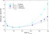 |
Fig. 19 Effect of a nonuniform outflow on the ratio
fesc(Lyα)/fesc(UV)
in the same clumpy shell geometry studied in Fig. 18 (FF = 0.23, CF = 0.997,
|

A high dust content has to be embedded in clumps: as explained in Sect. 3.2.2 and shown in Fig. 18, no enhancement of EW(Lyα) is found below a certain critical dust content (denoted τc in Fig. 6). A high dust content is indeed needed in the ISM to absorb UV continuum photons more efficiently than Lyα photons, which thus produces an enhancement of EW(Lyα). As shown in Fig. 18, a colour excess higher than E(B − V)Calzetti = 0.32 (i.e. τc ≈ 5) would be needed to enhance EW(Lyα) by a factor higher than 3. This dust content limit mainly depends on the covering factor CF of the ISM, where it decreases as CF decreases.
The distribution of the clumps around the stars: the spatial distribution of the clumps around the stars plays an important role in the enhancement of EW(Lyα). A covering factor CF close to unity is needed in order to get an enhancement of EW(Lyα) as high as those shown in Fig. 18. The enhancement of EW(Lyα) is indeed maximized when CF = 1, but it strongly decreases as CF decreases around the stars. A low covering factor CF does not allow more effectively blocking UV continuum photons than Lyα photons, thereby decreasing the enhancement of EW(Lyα). In particular, under the physical conditions adopted in Fig. 18, we notice that the enhancement of EW(Lyα) stays lower than 1.38 for CF ≲ 0.68.
In Figs. 18 and 19, the total Lyα flux is taken into account to derive the EW(Lyα) enhancement. However, an observer could measure a lower EW(Lyα) in practice if Lyα is scattered into an extended low surface brightness region, as recently observed around distant starburst galaxies (Steidel et al. 2011) or in nearby galaxies (Östlin et al. 2009).
Concerning the required dust extinction and the high density contrast of neutral
hydrogen (i.e.
nIC/nC<
10-7), these conditions seem more characteristic of molecular clouds
embedded in a very hot and ionized medium. The Neufeld model could therefore only work
in such a galactic environment. It is nevertheless interesting to notice that these
necessary conditions for an enhancement of EW(Lyα) in
a clumpy ISM are in perfect agreement with those originally predicted by Neufeld (1991). In his original paper, Neufeld indeed
proposed three suitable conditions for an enhancement of
EW(Lyα) in a clumpy ISM: the interclump medium (ICM)
must exhibit a very low density with a negligible small absorption and scattering
coefficients to Lyα photons, the clumpy ISM must show a large covering
factor (CF) and a sufficiently small volume filling factor that the ICM can “percolate”
(i.e. each part of the interclump medium must be connected to every other part), and the
probability for Lyα photons being reflected by the clumps must be
higher than the probability of being absorbed. In particular, this last probability
should increase when vexp decreases and
increases, which is consistent with our results. In addition to the criteria proposed by
Neufeld (1991), our work highlights the extreme
sensitivity of the Neufeld scenario to the kinematic of the clumps (i.e. the large-scale
outflows and the velocity dispersion of the clumps) and its strong dependence on the
dust content. Given the ubiquitous evidence of outflows from most star-forming galaxies
and the widespread presence of dust, it is essential to take these effects into account.
Furthermore, beyond the work of Neufeld (1991),
our detailed radiation transfer models including the Lyα line but also
transfer of continuum photons at other wavelengths, also allow us to predict the
resulting attenuation (reddening) and the detailed Lyα line profile
consistently, which can be compared directly to observations.
5.3. Studying the ISM through the Lyα line profile
Although the Lyα line profiles emerging both from homogeneous and clumpy ISMs are quite similar (Fig. 13), we have identified two main effects produced by the ISM clumpiness on the Lyα line profiles. First, we have seen that an extremely clumpy ISM favours the formation of a peak at the line centre of the line profile (vobs = 0 km s-1). Second, since Lyα escape is facilitated in a clumpy medium, the effect of the dust on the Lyα line profile is less efficient than in homogeneous media (Figs. 15 and 16). This can lead to intense Lyα emission emerging from a very dusty clumpy ISM, whereas an absorption line profile would emerge from a homogeneous medium with the same dust content.
This second effect of the ISM clumpiness on the Lyα line profiles can be
a source of uncertainties if we aim to derive some information on the ISM of distant
starburst galaxies (kinematics vexp, H i column
density ,
dust content )
from Lyα line fitting (Verhamme et al.
2008; Schaerer & Verhamme 2008).
Indeed, depending on either the homogeneity or clumpiness of the ISM, different derived
parameters of the ISM can be obtained by studying the same sample of galaxies. Among the
ISM parameters it is possible to derive from the fit of both the Lyα line
and the UV continuum (vexp,
,
),
the dust optical depth ()
seems the most uncertain parameter, given the dependence on the degree of clumping. On the
positive side, the expansion velocity may probably be best determined. In asymmetric
Lyα profiles the frequency of the second bump – if present – traces
2 × vexp quite well, both in homogeneous or clumpy media, as
already pointed out by Verhamme et al. (2006).
However, complications may be that two bumps (i.e. those located at the line centre and
those redshifted at 2 × vexp in Fig. 16) are not detectable (e.g. due to insufficient spectral resolution),
and the second bump (i.e. shifted at 2 × vexp) may not always
correspond to the peak of the profile. Also, depending on the column density, the
distinction of the two peaks may not be very easy (Verhamme et al. 2006).
In any case, compared to the typical Lyα line profiles observed in distant LAEs and LBGs, we note that most of them are asymmetric lines with redshifted peaks, which seem difficult to reconcile with the profiles predicted for very clumpy shell geometries, both static or expanding, since the peak is then expected to show negligible redshift. Furthermore, Lyα absorption lines are usually found among the reddest (presumably more dusty) LBGs, and the Lyα equivalent width correlates with reddening (e.g. Shapley et al. 2003), facts naturally explained by radiation transfer models with a homogenous ISM (Verhamme et al. 2008; Schaerer & Verhamme 2008). These findings also argue against a very clumpy, high-contrast ISM, at least for the majority of LBGs.
5.4. Comparison with Hansen & Oh (2006)
We now compare our results with the recent numerical study of Lyα
transfer in multiphase and dusty media from Hansen
& Oh (2006, hereafter HO06). The
clumpy media studied in HO06 are only extremely clumpy, which are composed of very
optically thick spherical clumps (H i + dust) distributed within an empty
interclump medium. From such clumpy media, HO06 deduce analytical formulae fitting the
behaviour of both the continuum and the Lyα escape fractions as a
function of gas geometry, motion, and dust content. In summary, assuming an isotropic
scattering by dust grains (g = 0) in optically thick spherical clumps,
the fitting formula is a function of two parameters (Eq. (59) in HO06):
 (15)where
N0 (a geometrical parameter) corresponds to the average
number of clumps encountered by photons before escaping the medium in the absence of
absorption, and where ϵc(ν) (a dust
parameter) corresponds to the probability of a photon of frequency ν to
be absorbed rather than reflected by a clump. In the clumpy shell geometries of our model,
both parameters can be derived in the following way. Firstly, we notice that
N0 tends to evolve as
N0 = 1.1fc2 +
1.42fc, where fc corresponds to the mean number of
clumps intersected along a random line of sight. The parameter
ϵc(ν) can be estimated simply using the
formula derived in HO06 (Eq. (27) of their paper):
(15)where
N0 (a geometrical parameter) corresponds to the average
number of clumps encountered by photons before escaping the medium in the absence of
absorption, and where ϵc(ν) (a dust
parameter) corresponds to the probability of a photon of frequency ν to
be absorbed rather than reflected by a clump. In the clumpy shell geometries of our model,
both parameters can be derived in the following way. Firstly, we notice that
N0 tends to evolve as
N0 = 1.1fc2 +
1.42fc, where fc corresponds to the mean number of
clumps intersected along a random line of sight. The parameter
ϵc(ν) can be estimated simply using the
formula derived in HO06 (Eq. (27) of their paper):
 (16)with
ϵ(ν) as the absorption probability per interaction
(H I or dust) at frequency ν. In particular,
ϵ(ν) is thus given by
ϵ(ν) = 1 − a for the UV
continuum photons, with a the dust albedo.
(16)with
ϵ(ν) as the absorption probability per interaction
(H I or dust) at frequency ν. In particular,
ϵ(ν) is thus given by
ϵ(ν) = 1 − a for the UV
continuum photons, with a the dust albedo.
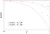 |
Fig. 20 Test of Eq. (15) of HO06. We show here the evolution of the UV escape fraction from two different extremely clumpy shell geometries as a function of the absorption parameter ϵc. The first medium (square dots) shows N0 = 1.00 and is built with FF = 0.10, CF = 0.38, and nIC/nC = 0. The second medium (circle dots) shows N0 = 4.28 and is built with FF = 0.15, CF = 0.70, and nIC/nC = 0. In both media, each clump is opaque to dust extinction. The clumps are therefore optically thick for UV continuum photons. Both full lines represent the Eq. (15) for N0 = 1.00 (top line) and N0 = 4.28 (bottom line), respectively. |
We compare in Fig. 20 the Eq. (15) (full lines) to the UV continuum escape fraction derived from the clumpy shell geometries of our model (grey dots). In this figure, two clumpy shell geometries are studied. The first structure, built with FF = 0.10, CF = 0.38 and nIC/nC = 0, shows N0 = 1.0 (top line). The second structure, assuming FF = 0.15, CF = 0.70, and nIC/nC = 0, shows N0 = 4.28 (bottom line). In Fig. 20, we just change the values of ϵc(ν) by changing the albedo a of the dust grains, as shown in Eq. (16). Although a certain difference appears as ϵc tends towards 1, the continuum escape fraction deduced from our numerical simulations are rather well fitted by the analytical formula of HO06 (Eq. (15)). In particular, the UV escape fraction follows the same dependence on N0 and ϵc as predicted by Eq. (15) for the low-absorption regime (ϵc < 0.4). The difference observed close to ϵc = 1 is also observed in HO06 and is explained by a geometrical effect. As suggested by these authors, a better fit can be obtained in this regime by rescaling the term ϵc(ν)N0 (Eq. (15)) as κϵc(ν)N0, where κ is a unity fitting parameter.
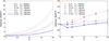 |
Fig. 21 Evolution of the Lyα line-to-continuum escape fractions ratio,
fesc(Lyα)/fesc(UV),
as a function of the dust optical depth |
Although our numerical simulations reproduce all the results and the fitting formula of
HO06 reasonably well, our conclusions diverge from theirs concerning the Neufeld model. As
an application of their numerical study, HO06 give a quantitative estimation of the
EW(Lyα) enhancements produced by different clumpy and
dusty ISMs (Fig. 18 of their paper). We reproduce the results of HO06 in Fig. 21 (left panel). These results are based on the
following assumptions concerning the clumpy media: 1) the clumps are extremely opaque to
Lyα photons; but 2) each clump is not opaque to dust extinction (i.e.
the total dust optical depth for a single clump, considering that the effect of scattering
plus absorption is τd < 1)2, rendering each clump optically thin for UV continuum
photons. Given these assumptions, HO06 adopt a constant value of
fesc(Lyα) (derived by an analytical method
based on Eq. (15)), whereas the UV continuum escape fraction is assumed to behave like in
homogeneous media. In a homogenous medium composed of dust grains with an albedo
ϵd ≈ 0.5, the UV escape fraction is approximately given by
the following equation: 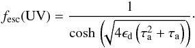 (17)In
the right-hand panel of Fig. 21 we show the results
obtained by studying the same media than HO06 (i.e. six clumpy media constructed with
three different values of N0 = 1, 4, and 10), but using our
own numerical approach. In particular, we derive each curve of the right-hand panel
studying the real evolution of fesc(UV) and
fesc(Lyα) with full Monte Carlo
simulations. We can clearly see that we cannot reproduce, whether quantitatively or
qualitatively, the curves of HO06. This strong difference is explained by both assumptions
made by HO06 on fesc(UV) (i.e. Eq. (17)) and
fesc(Lyα) (i.e. a constant value under any
dust optical depth ),
which cannot be rigorously met in any clumpy media constructed with low values of
N0, as studied in Fig. 21. We compare in Fig. 22 the UV and
Lyα escape fractions deduced from our simulations to the assumptions
made in HO06. Firstly, while HO06 use the Eq. (17) to deduct the evolution of
fesc(UV) as a function of
(i.e.
fesc(UV) is therefore assumed to behave like in homogeneous
media, which is only correct if the clumpy media are composed of enough optically
thin clumps distributed in a way they can intersect all line of sights
around the stars), this assumption clearly underestimates the correct values of
fesc(UV) in the clumpy media studied in Fig. 21. This discrepancy is explained by the fact that those
clumpy media are composed of very few clumps that cannot intersect all line of sights
around the photon sources3. Furthermore, this small
number of clumps prevent them from staying optically thin to dust extinction in the range
of
[0:2]. As a consequence, a large fraction of UV continuum photons can directly escape the
clumpy media through several free spaces that appear between clumps, preventing
fesc(UV) from behaving like in homogeneous media (i.e. Eq.
(17)). Secondly, the constant values of
fesc(Lyα) assumed by HO06 from their Eq.
(15) tend to overestimate those obtained from our simulations. This second discrepancy is
mainly explained by fesc(Lyα) always
increasing as the dust optical depth
decreases in any clumpy media.
(17)In
the right-hand panel of Fig. 21 we show the results
obtained by studying the same media than HO06 (i.e. six clumpy media constructed with
three different values of N0 = 1, 4, and 10), but using our
own numerical approach. In particular, we derive each curve of the right-hand panel
studying the real evolution of fesc(UV) and
fesc(Lyα) with full Monte Carlo
simulations. We can clearly see that we cannot reproduce, whether quantitatively or
qualitatively, the curves of HO06. This strong difference is explained by both assumptions
made by HO06 on fesc(UV) (i.e. Eq. (17)) and
fesc(Lyα) (i.e. a constant value under any
dust optical depth ),
which cannot be rigorously met in any clumpy media constructed with low values of
N0, as studied in Fig. 21. We compare in Fig. 22 the UV and
Lyα escape fractions deduced from our simulations to the assumptions
made in HO06. Firstly, while HO06 use the Eq. (17) to deduct the evolution of
fesc(UV) as a function of
(i.e.
fesc(UV) is therefore assumed to behave like in homogeneous
media, which is only correct if the clumpy media are composed of enough optically
thin clumps distributed in a way they can intersect all line of sights
around the stars), this assumption clearly underestimates the correct values of
fesc(UV) in the clumpy media studied in Fig. 21. This discrepancy is explained by the fact that those
clumpy media are composed of very few clumps that cannot intersect all line of sights
around the photon sources3. Furthermore, this small
number of clumps prevent them from staying optically thin to dust extinction in the range
of
[0:2]. As a consequence, a large fraction of UV continuum photons can directly escape the
clumpy media through several free spaces that appear between clumps, preventing
fesc(UV) from behaving like in homogeneous media (i.e. Eq.
(17)). Secondly, the constant values of
fesc(Lyα) assumed by HO06 from their Eq.
(15) tend to overestimate those obtained from our simulations. This second discrepancy is
mainly explained by fesc(Lyα) always
increasing as the dust optical depth
decreases in any clumpy media.
In conclusion, the assumptions of HO06 clearly underestimate the correct values of
fesc(UV) and overestimate those of
fesc(Lyα). This explains why the
enhancements of EW(Lyα) obtained in HO06 (left panel in
Fig. 21) are much higher than those deduced from our
simulations (right panel). Furthermore, the right-hand panel shows the inversion of the
curves (in terms of N0) as
increases. The highest enhancement of EW(Lyα) is indeed
produced by clumpy media containing the highest number of clumps around stars.
Drawing the parallel with our study of the Neufeld scenario in Sect. 5.2, we notice that most of the models showing an enhancement of EW(Lyα) in Fig. 21 (right panel) respect all conditions quite well under which the Neufeld scenario works in a clumpy ISM: 1) the interclump medium is optically thin for Lyα photons (nIC/nC = 0); 2) the expansion velocities vexp are slow and uniform; and 3) the enhancements of EW(Lyα) occur above a certain dust optical depth τc equal to (0, 0, 0.3) in all clumpy media (N0 = 1,4,10). Furthermore, as expected when an enhancement of EW(Lyα) occurs in a clumpy ISM, the Lyα line profiles emerging from each clumpy geometry studied in Fig. 21 are symmetric and peaked at the line centre.
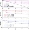 |
Fig. 22 Predicted UV and Lyα escape fraction as a function of
|
5.5. Recent models of Lyα transfer in clumpy large-scale outflows
Recently Dijkstra & Kramer (2012) have presented radiative transfer calculations of Lyα photons propagating through clumpy, dusty, large-scale outflows using phenomenologically motivated models constrained by absorption line measurement from Steidel et al. (2011). The calculations of Dijkstra & Kramer mostly focus on the Lyα surface brightness distribution. However, since their calculations do not follow the behaviour of the UV continuum, it is not possible to infer any information on the presence or absence of an efficient “Neufeld effect”. Furthermore, the Lyα line profiles predicted by their models are not presented. It is therefore not possible to compare our results with the calculations of Dijkstra & Kramer (2012) or to compare their model to the most direct and sensitive observable, the Lyα line profile itself.
6. Summary and conclusions
To examine and understand the effects of clumpy ISM structures on the Lyα line and UV observations of star-forming galaxies we carried out detailed radiation transfer calculations using our 3D Lyα Monte Carlo code MCLyα (Verhamme et al. 2006; Schaerer et al. 2011). Indeed, clumping can in principle significantly alter the transfer of Lyα in galaxies, as shown early by Neufeld (1991), and has often been invoked to explain strong Lyα emission or a higher transmission for Lyα photons than for the UV continuum (e.g. Kudritzki et al. 2000; Malhotra & Rhoads 2002; Rhoads et al. 2003; Shimazaku et al. 2006). However, only a few detailed numerical studies of these effects have so far been undertaken (Haiman & Spaans 1999; Richling 2003; Hansen & Oh 2006; Laursen et al. 2013), albeit with some simplifying assumptions in most of these works. Furthermore, we wish to identify in which conditions clumping affects the line transfer and how much, and how, this is reflected in the emergent Lyα line profiles.
Our radiation transfer calculations allow us to simultaneously study the dependence of both the Lyα and the continuum escape fractions, the Lyα equivalent width EW(Lyα), and the Lyα line profiles on the H i content, the dust content, kinematics, gas geometry, and clumping properties. Since spherically symmetric outflows with a homogeneous H i shell are able to reproduce a wide variety of observed Lyα line profiles in Lyman break galaxies and LAEs (Verhamme et al. 2008; Schaerer & Verhamme 2008; Dessauges-Zavadsky et al. 2010), the same geometry is used to study how a clumpy ISM structure alters the Lyα line and UV continuum. This clumpy geometry is also chosen since it has been shown to reproduce observable continuum properties of starburst galaxies and the Calzetti attenuation law (Gordon et al. 1997; Witt & Gordon 2000; Vijh et al. 2003).
Our main results can be summarized as follows:
-
A clumpy and dusty medium is always more transparent toLy α, UV, and optical continuum photons than is an equivalent homogeneous medium of equal dust content, as alreadyknown from earlier studies (Boisse 1990; Hobson &Scheuer 1993; Witt &Gordon 1996, 2000). A clumpymedium thus allows decreasing the overall effect of the dustabsorption on any radiation.
-
The UV and optical continuum escape fraction depend on three parameters in homogeneous and clumpy shell geometries: the dust content, the “clumpiness” of the dust distribution (described by the density contrast n IC/n C), and the covering factor CF (defined here as the fraction of solid angle of the central photons source covered by the clumps). In a general way, the continuum escape fraction decreases as the clumpiness of the dust distribution decreases (i.e. n IC/n C increases), and as both the dust content and the covering factor increase.
-
Three additional parameters, i.e. in total six, control the Lyα line transfer: the dust content, the density contrast nIC/nC, the covering factor, as well as the H i column density, the velocity field, and the gas temperature. The Lyα escape fraction always increases when increasing the clumpiness (i.e. nIC/nC decreases), and with decreasing dust content and covering factor. However, the H i column density and the kinematics of the gas do not affect the Lyα escape in the same way for homogeneous or clumpy media. That creates two different regimes for the Lyα radiative transfer in clumpy media.
-
The first regime (called low-contrast regime in this paper) comprises homogeneous and weakly clumpy shell geometries, corresponding to an interclump density above nIC/nC ≳ 1.5 × 10⁻⁴ for the physical conditions adopted in our model (such that the interclump medium is also optically thick for Lyα). In this regime, the Lyα escape fraction increases with increasing expansion velocity vexp and with decreasing H i column density
,
as for a homogenous ISM. The Lyα escape
fraction is then always less than or equal to the UV escape fraction, which implies
that the emergent Lyα equivalent width
EWobs(Lyα)
is lower than the intrinsic one
EWint(Lyα).
-
The second regime (called high-contrast regime) is found in the most extremely clumpy shell geometries of our model (nIC/nC ≲ 1.5 × 10⁻⁴ for the physical conditions adopted in our model). This corresponds to a clumpy medium composed of very dense clumps embedded in an interclump region that is optically thin for Lyα photons. Two main differences appear compared to the other regime. First, as was originally suggested by Neufeld (1991), it is possible to observe a Lyα escape fraction that is higher than for the UV continuum. In particular, this is possible above a certain “critical” dust optical depth τc. Second, whereas for
 the
Lyα escape fraction behaves as in the
low-contrast regime, the opposite behaviour is found for high enough dust content
(
the
Lyα escape fraction behaves as in the
low-contrast regime, the opposite behaviour is found for high enough dust content
( ), where
fesc(Lyα) increases with
decreasingvexp
andincreasing .
), where
fesc(Lyα) increases with
decreasingvexp
andincreasing .
-
Overall we have identified two main effects of the ISM clumpiness on the shape of the Lyα line profiles. First, extremely clumpy ISM favours the formation of a peak at the centre of the line profile (vobs = 0). Second, the intensity of the Lyα line increases as the clumpiness of the medium increases, as expected.
-
Schematically, the following Ly α line profile morphologies are predicted from homogeneous and clumpy shell geometries: “double-peak” profiles with identical/similar peaks symmetric around the source redshift (for static media), asymmetric redshifted profiles (from expanding media), and absorption line profiles (from very dusty, homogeneous, or weakly clumpy media). These types have already been identified in homogenous models (Verhamme et al. 2006). In very clumpy, static, and dusty shells, a new category is found: “three peak” profiles similar to the double-peak profiles with an additional third component at line centre.
As an application of our study, we have examined the conditions under which the Neufeld model (Neufeld 1991) can work in a clumpy ISM, i.e. when an enhancement of the observed EWobs(Lyα) can be obtained. We find that the following five conditions must be simultaneously fulfilled for the “Neufeld” effect to be effective.
-
The H i content must be verylow between clumps, typically theH i column density in theinterclump region must be ≲3 × 1014 cm-2 to remain optically thin for Lyα photons. Otherwise, Lyα photons scatter strongly against H i atoms localized between clumps and cannot escape the clumpy medium more easily than UV photons.
-
The galactic outflow has to be slow with outflow velocities of the order of vexp ≲ 2 × FWHMint(Lyα) km s-1. Otherwise Lyα photons are too redshifted from the clumps and can no longer scatter on the surface of clumps, as suggested in the Neufeld model.
-
The galactic outflow has to be as uniform and constant as possible in velocity for efficient interactions of Lyα photons with dust.
-
A high dust content must be embedded in clumps to absorb the UV continuum as much as possible, which increases the Lyα equivalent width. For the physical conditions and clumpy shell geometries adopted here, we find that an enhancement of EW(Lyα) by a factor 3–4 can only occur for a colour excess E(B − V) ≳ 0.3.
-
A large covering factor is needed in order to get a noticeable enhancement of EW (Lyα).
The above conditions agree with the general findings of Neufeld (1991). However, our results differ from those of Hansen & Oh (2006), who make some simplifying assumptions that are not consistent with more rigorous radiation transfer calculations. In our study, the Neufeld model does not work as easily as suggested in Hansen & Oh (2006).
Given our results it seems quite unlikely, or even difficult, to find conditions in a clumpy, spherically symmetric ISM, where Lyα photons can escape more easily than in the nearby UV continuum, i.e. where the phenomenon suggested by Neufeld (1991) can be at play. Furthermore, when these conditions are fulfilled we generally find that the emergent Lyα line profile shows emission at line centre and little asymmetry. Such profiles do not, however, represent the profiles typically observed in high-redshift galaxies, which are known to be redshifted in the galaxy rest-fame and asymmetric. Other arguments against the Neufeld effect being effective may be if the sites of Lyα emission are relatively close to or within cold, dusty environments such as molecular clouds, which could absorb Lyα photons more efficiently than the UV continuum (Laursen et al. 2013; Verhamme et al. 2012).
The simulations from this paper and the success of homogenous, spherically expanding models in reproducing the wide variety of observed Lyα line profiles and velocity shifts between photospheric, low ionization absorption, and the Lyα line (Verhamme et al. 2008; Schaerer & Verhamme 2008) seems to indicate that the effects of the inhomogeneities in the ISM and deviations from spherical geometry are not dominant. Why simple geometries work so well may appear somewhat puzzling, and certainly remains worth understanding in more depth. More detailed observations and sophisticated radiation transfer models within multi-phase ISM, high-resolution simulations may help shed more light on this question and help examine how well the physical parameters derived from Lyα line profile fits using simple spherically expanding model represent reality.
The optical depth at line centre is  (12.85 km s-1/b) NHI, e.g.
Verhamme et al. (2006).
(12.85 km s-1/b) NHI, e.g.
Verhamme et al. (2006).
Nevertheless, the total dust optical depth across the entire clumpy medium can be greater than unity if many clumps are intersected along the radius of the medium.
All clumpy media showing N0 ≤ 10 always have a covering factor CF < 0.90.
Acknowledgments
We thank Anne Verhamme for interesting comments on an earlier version of this paper. Simulations were done on the regor PC cluster at the Geneva Observatory co-funded by grants to Georges Meynet, Daniel Pfenniger, and D.S. The work of D.S. was supported by the Swiss National Science Foundation. Peter Laursen acknowledges support from the ERC-StG grant EGGS-278202.
References
- Ahn, S.-H., Lee, H.-W., & Lee, H. M. 2001, AJ, 554, 604 [Google Scholar]
- Ahn, S.-H., Lee, H.-W., & Lee, H. M. 2002, AJ, 567, 920 [Google Scholar]
- Ahn, S.-H., Lee, H.-W., & Lee, H. M. 2003, MNRAS, 340, 863 [NASA ADS] [CrossRef] [Google Scholar]
- Atek, H., Kunth, D., Hayes, M., Östlin, G., & Mas-Hesse, J. M. 2008, A&A, 488, 491 [NASA ADS] [CrossRef] [EDP Sciences] [Google Scholar]
- Atek, H., Schaerer, D., & Kunth, D. 2009, A&A, 502, 791 [NASA ADS] [CrossRef] [EDP Sciences] [Google Scholar]
- Baker, A. J., Tacconi, L. J., Genzel, R., Lehnert, M. D., & Lutz, D. 2004, ApJ, 604, 125 [NASA ADS] [CrossRef] [Google Scholar]
- Boisse, P. 1990, A&A, 228, 483 [NASA ADS] [Google Scholar]
- Calzetti, D. 1997, ApJ, 113, 162 [Google Scholar]
- Calzetti, D., Armus, L., Bohlin, R. C., et al. 2000, ApJ, 533, 682 [NASA ADS] [CrossRef] [Google Scholar]
- Cantalupo, S., Porciani, C., Lilly, S. J., & Miniati, F. 2005, AJ, 628, 61 [Google Scholar]
- Charlot, S., & Fall, S. M. 1993, ApJ, 415, 580 [NASA ADS] [CrossRef] [Google Scholar]
- Cowie, L. L., & Hu, E. M. 1998, AJ, 115, 1319 [NASA ADS] [CrossRef] [Google Scholar]
- Dawson, S., Rhoads, J. E., Malhotra, S., et al. 2004, AJ, 617, 707 [Google Scholar]
- Dayal, P., Ferrara, A., Saro, A., et al. 2009, MNRAS, 400, 2000 [NASA ADS] [CrossRef] [Google Scholar]
- Dessauges-Zavadsky, M., D’Odorico, S., Schaerer, D., et al. 2010, A&A, 510, A26 [NASA ADS] [CrossRef] [EDP Sciences] [Google Scholar]
- Dickey, J. M., & Garwood, R. W. 1989, ApJ, 341, 201 [NASA ADS] [CrossRef] [Google Scholar]
- Dijkstra, M., & Kramer, R. H. 2012, MNRAS, 386, 1 [Google Scholar]
- Erb, D. K., Shapley, A. E., Steidel, C. C., et al. 2003, ApJ, 591, 101 [NASA ADS] [CrossRef] [Google Scholar]
- Fan, X., Narayanan, V. K., Strauss, M. A., et al. 2002, AJ, 123, 1247 [NASA ADS] [CrossRef] [Google Scholar]
- Finkelstein, S. L., Rhoads, J. E., Malhotra, S., Grogin, N., & Wang, J. 2008, ApJ, 678, 655 [NASA ADS] [CrossRef] [Google Scholar]
- Finkelstein, S. L., Rhoads, J. E., Malhotra, S., & Grogin, N. 2009, ApJ, 691, 465 [NASA ADS] [CrossRef] [Google Scholar]
- Forero-Romero, J. E., Yepes, G., Gottlber, S., et al. 2011, MNRAS, 415, 3666 [NASA ADS] [CrossRef] [Google Scholar]
- Gawiser, E., van Dokkum, P. G., Gronwall, C., et al. 2006, AJ, 642, L13 [Google Scholar]
- Giavalisco, M., Koratkar, A., & Calzetti, D. 1996, ApJ, 466, 831 [NASA ADS] [CrossRef] [Google Scholar]
- Gordon, K. D., Calzetti, D., & Witt, A. N. 1997, ApJ, 487, 625 [NASA ADS] [CrossRef] [Google Scholar]
- Gronwall, C., Ciardullo, R., Hickey, T., et al. 2007, ApJ, 667, 79 [NASA ADS] [CrossRef] [Google Scholar]
- Guaita, L., Gawiser, E., Padilla, N., et al. 2010, ApJ, 714, 255 [NASA ADS] [CrossRef] [Google Scholar]
- Haiman, Z., & Spaans, M. 1999, ApJ, 518, 138 [NASA ADS] [CrossRef] [Google Scholar]
- Hansen, M., & Oh, S. P. 2006, New Astron. Rev., 367, 979 [Google Scholar]
- Hayes, M., & Östlin, G. 2006, A&A, 460, 681 [NASA ADS] [CrossRef] [EDP Sciences] [Google Scholar]
- Hobson, M. P., & Scheuer, P. A. G. 1993, MNRAS, 264, 145 [NASA ADS] [Google Scholar]
- Hu, E. M., Cowie, L. L., & McMahon, R. G. 1998, ApJ, 502, L99 [NASA ADS] [CrossRef] [Google Scholar]
- Hu, E. M., Cowie, L. L., Capak, P., et al. 2004, ApJ, 127, 563 [Google Scholar]
- Kashikawa, N., Shimasaku, K., Malkan, M. A., et al. 2006, ApJ, 648, 7 [NASA ADS] [CrossRef] [Google Scholar]
- Kashikawa, N., Nagao, T., Toshikawa, J., et al. 2012, ApJ, 761, 85 [NASA ADS] [CrossRef] [Google Scholar]
- Kudritzki, R.-P., Méndez, R. H., Feldmeier, J. J., et al. 2000, ApJ, 536, 19 [NASA ADS] [CrossRef] [Google Scholar]
- Kunth, D., Lequeux, J., Sargent, W. L. W., & Viallefond, F. 1994, A&A, 282, 709 [NASA ADS] [Google Scholar]
- Kunth, D., Mas-Hesse, J. M., Terlevich, E., et al. 1998, A&A, 334, 11 [NASA ADS] [Google Scholar]
- Laursen, P., Razoumov, A. O., & Sommer-Larsen, J. 2009a, ApJ, 696, 853 [Google Scholar]
- Laursen, P., Sommer-Larsen, J., & Andersen, A. C. 2009b, ApJ, 704, 1640 [NASA ADS] [CrossRef] [Google Scholar]
- Laursen, P., Duval, F., & Östlin, G. 2013, ApJ, 766, 124 [NASA ADS] [CrossRef] [Google Scholar]
- Lequeux, J., Kunth, D., Mas-Hesse, J. M., & Sargent, W. L. W. 1995, A&A, 301, 18 [NASA ADS] [Google Scholar]
- Malhotra, S., & Rhoads, J. E. 2002, ApJ, 565, L71 [NASA ADS] [CrossRef] [Google Scholar]
- Malhotra, S., & Rhoads, J. E. 2004, ApJ, 617, L5 [NASA ADS] [CrossRef] [Google Scholar]
- Marscher, A. P., Moore, E. M., & Bania, T. M. 1993, AJ, 419, 101 [Google Scholar]
- Mas-Hesse, J. M., Kunth, D., Tenorio-Tagle, G., et al. 2003, ApJ, 598, 858 [NASA ADS] [CrossRef] [Google Scholar]
- McKee, C. F., & Ostriker, J. P. 1977, ApJ, 218, 148 [NASA ADS] [CrossRef] [Google Scholar]
- McLinden, E. M., Finkelstein, S. L., Rhoads, J. E., et al. 2011, ApJ, 730, 136 [NASA ADS] [CrossRef] [Google Scholar]
- Meier, D. L., & Terlevich, R. 1981, AJ, 246, 109 [Google Scholar]
- Neufeld, D. A. 1990, ApJ, 350, 216 [NASA ADS] [CrossRef] [Google Scholar]
- Neufeld, D. A. 1991, ApJ, 370, L85 [NASA ADS] [CrossRef] [Google Scholar]
- Nilsson, K. K., Møller, P., Möller, O., et al. 2007, A&A, 471, 71 [NASA ADS] [CrossRef] [EDP Sciences] [Google Scholar]
- Östlin, G., Hayes, M., Kunth, D., et al. 2009, ApJ, 138, 923 [Google Scholar]
- Ouchi, M., Shimasaku, K., Furusawa, H., et al. 2003, ApJ, 582, 60 [NASA ADS] [CrossRef] [Google Scholar]
- Ouchi, M., Shimasaku, K., Akiyama, M., et al. 2008, ApJS, 176, 301 [NASA ADS] [CrossRef] [Google Scholar]
- Ouchi, M., Shimasaku, K., Furusawa, H., et al. 2010, ApJ, 723, 869 [NASA ADS] [CrossRef] [Google Scholar]
- Partridge, R., & Peebles, P. J. E. 1967, ApJ, 147, 868 [NASA ADS] [CrossRef] [Google Scholar]
- Pierleoni, M., Maselli, A., & Ciardi, B. 2007 [Google Scholar]
- Rhoads, J. E., Dey, A., Malhotra, S., et al. 2000, ApJ, 545, 85 [Google Scholar]
- Rhoads, J. E., Dey, A., Malhotra, S., et al. 2003, AJ, 125, 1006 [NASA ADS] [CrossRef] [Google Scholar]
- Richling, S. 2003, MNRAS, 344, 553 [NASA ADS] [CrossRef] [Google Scholar]
- Santos, M.R. 2004, Galaxy formation near the epoch of reionization, TeXbook (CaltechTHESIS) [Google Scholar]
- Scarlata, C., Colbert, J., Teplitz, H. I., et al. 2009, ApJ, 704, 98 [Google Scholar]
- Schaerer, D. 2003, A&A, 397, 527 [NASA ADS] [CrossRef] [EDP Sciences] [Google Scholar]
- Schaerer, D., & Verhamme, A. 2008, A&A, 480, 369 [NASA ADS] [CrossRef] [EDP Sciences] [Google Scholar]
- Schaerer, D., Hayes, M., Verhamme, A., & Teyssier, R. 2011, A&A, 531, A12 [NASA ADS] [CrossRef] [EDP Sciences] [Google Scholar]
- Shimasaku, K., Kashikawa, N., Doi, M., et al. 2006, PASJ, 58, 313 [NASA ADS] [Google Scholar]
- Steidel, C. C., Bogosavljevic, M., Shapley, A. E., et al. 2011, ApJ, 736, 160 [NASA ADS] [CrossRef] [Google Scholar]
- Stutzki, J., & Guesten, R. 1990, AJ, 256, 513 [NASA ADS] [CrossRef] [Google Scholar]
- Swinbank, A. M., Papadopoulos, P. P., Cox, P., et al. 2011, AJ, 742, 11 [NASA ADS] [CrossRef] [Google Scholar]
- Taniguchi, Y., Ajiki, M., Murayama, T., & Nagao, T. 2003, ApJ, 585, L97 [NASA ADS] [CrossRef] [Google Scholar]
- Taniguchi, Y., Ajiki, M., Nagao, T., et al. 2005, PASJ, 57, 165 [NASA ADS] [Google Scholar]
- Tenorio-Tagle, G., Silich, S. A., Kunth, D., Terlevich, E., & Terlevich, R. 1999, MNRAS, 309, 332 [NASA ADS] [CrossRef] [Google Scholar]
- Teplitz, H. I., McLean, I. S., Becklin, E. E., et al. 2000, ApJ, 533, L65 [NASA ADS] [CrossRef] [PubMed] [Google Scholar]
- Thuan, T. X., Izotov, Y. I., & Lipovetsky, V. A. 1997, ApJ, 477, 661 [NASA ADS] [CrossRef] [Google Scholar]
- Varosi, F., & Dwek, E. 1999 [arXiv:astro-ph/9905291] [Google Scholar]
- Verhamme, A., Schaerer, D., & Maselli, A. 2006, A&A, 460, 397 [NASA ADS] [CrossRef] [EDP Sciences] [Google Scholar]
- Verhamme, A., Schaerer, D., Atek, H., & Tapken, C. 2008, A&A, 491, 89 [NASA ADS] [CrossRef] [EDP Sciences] [Google Scholar]
- Verhamme, A., Dubois, Y., Blaizot, J., et al. 2012, A&A, 546, A111 [NASA ADS] [CrossRef] [EDP Sciences] [Google Scholar]
- Vijh, U. P., Witt, A. N., & Gordon, K. D. 2003, AJ, 587, 533 [CrossRef] [Google Scholar]
- Wang, J. X., Rhoads, J. E., Malhotra, S., et al. 2004, AJ, 608, 21 [Google Scholar]
- Witt, A. N., & Gordon, K. D. 1996, ApJ, 463, 681 [NASA ADS] [CrossRef] [Google Scholar]
- Witt, A. N., & Gordon, K. D. 2000, ApJ, 528, 799 [Google Scholar]
All Tables
Six input parameters (top) for and derived parameter (bottom) of the homogeneous and clumpy shell models.
Dust parameters (a and g) taken from Witt & Gordon (2000) and adopted for Lyα line photons, and continuum photons at UV and optical wavelengths (close to the B and V-band).
Range of values of the six input parameters (Cols. 1–6) describing the homogeneous and clumpy shell models, and derived properties (Cols. 7, 8).
All Figures
|
Fig. 1 Representation of some 3D homogeneous and clumpy geometries studied in this paper. The star distribution is always localized in the centre of the shell, whereas the dust and the H i content are distributed around. The dust and H i distribution can be “homogeneous” (left), “clumpy” (middle) or “extremely clumpy” (right). In a “clumpy” distribution, the clumps and the interclump medium receive, respectively, high and low densities of dust and HI. In the case of an “extremely clumpy” distribution, all the dust and the H i content are distributed in clumps. |
| In the text | |
|
Fig. 2 Variation in clump size by adopting different filling factors FF in a shell geometry defined with Rmin = 49 and Rmax = 64 cells. The filling factors used here are FF = 0.07 (circles), FF = 0.13 (diamonds), and FF = 0.23 (triangles). The mass spectrum obtained with FF = 0.23 (ρ(m) ∝ m-2.04) is the most consistent with observations of diffuse interstellar clouds. We thus adopt FF = 0.23 throughout this study. |
| In the text | |
|
Fig. 3 Comparison of the UV-to-optical continuum escape fraction derived from our code with the results of Witt & Gordon (2000). The clumpy shell geometry studied here is built on a Cartesian grid of N = 303 cells and is characterized by the following parameters: FF = 0.15, nIC/nC = 0.01, Rmin = 5, and Rmax = 15. The evolution of the escape fraction at 25 different wavelengths is shown, from λ = 0.1 μm to λ = 30 μm, assuming three different dust optical depths τV in the shell structure (measured in V band): τV = 2, 4.5, and 8. The escape fractions obtained with MCLyα are marked in red, whereas those obtained by Witt & Gordon (2000) are marked in grey. We find very good agreement with Witt & Gordon (2000). |
| In the text | |
|
Fig. 4 Evolution of the UV escape fraction fesc(UV) as a
function of the dust optical depth ( |
| In the text | |
|
Fig. 5 Schematic representation of how UV continuum (red) and Lyα photons (blue) propogate in the low-contrast regime. The medium illustrated here is composed of high-density clumps (containing H i + dust), distributed in an interclump medium of low density (HI+dust). In the low-contrast regime, the H i content in and between clumps are relatively high, which renders both regions optically thick for the Lyα photons. In this way, the Lyα photons can only escape the medium after undergoing multiple resonant scattering against H i atoms, increasing their probability being absorbed by the dust. The UV photons are not affected by the presence of H i atoms and propagate directly through the medium. |
| In the text | |
|
Fig. 6 Evolution of the Lyα (blue lines) and UV continuum (red) escape
fraction as a function of the dust optical depth
( |
| In the text | |
|
Fig. 7 Evolution of the Lyα escape fraction
fesc(Lyα) as a function of dust
optical depth |
| In the text | |
|
Fig. 8 Schematic representation of the way the UV continuum (red) and the Lyα (blue) photons propogate in the high-contrast regime. The medium illustrated here is composed of high-density clumps (H i + dust), distributed in an empty interclump medium. A fraction of the Lyα photons scatter on the H i atom comprising the surface of the clumps. The rest of the Lyα photons, as well as the UV continuum photons, pierce the clumps where they may be absorbed by dust. |
| In the text | |
|
Fig. 9 Lyα (blue lines) and UV (red lines) escape fraction as a
function of the dust optical depth |
| In the text | |
|
Fig. 10 Lyα (blue lines) and UV (red line) escape fractions as a
function of the dust optical depth |
| In the text | |
|
Fig. 11 Evolution of the critical ratio nIC/nC separating the low-contrast regime from the high-contrast regime of the Lyα radiative transfer in clumpy shell geometries. For highest ratio nIC/nC, all clumpy media belong to the low-contrast regime, whereas for lower nIC/nC the high-contrast regime is observed. Three curves are represented in this figure corresponding to the three different physical conditions applied to our clumpy media (see text). |
| In the text | |
|
Fig. 12 Same as in Fig. 11, but showing the evolution
of the H i column density between clumps
NHI,IC (= (1 – FF)
× nICL, with L as the physical size of the shell), as
a function of the total |
| In the text | |
|
Fig. 13 Comparison between the Lyα line profiles emerging dust free
homogeneous shell (dotted blue lines), weakly clumpy shell (dashed magenta lines)
and extremely clumpy shells (thick red lines) under different expansion velocities
vexp. All homogeneous and clumpy shells have for
common parameters: |
| In the text | |
|
Fig. 14 Effect of the covering factor CF on the Lyα line profiles in
extremely clumpy shell geometries. We study here a static, extremely clumpy shell
geometry defined with the following parameters: FF = 0.23,
nIC/nC = 0.00,
|
| In the text | |
|
Fig. 15 Effects of the dust optical depth |
| In the text | |
|
Fig. 16 Same as Fig. 15 but for an expanding shell with vexp = 300 km s-1. No boost of Lyα with respect to the continuum is found in any of these models, since the expansion velocity is too high. Discussion in the text. |
| In the text | |
|
Fig. 17 Evolution of the colour excess
E(B − V) as a function of
|
| In the text | |
|
Fig. 18 Evolution of the ratio
fesc(Lyα)/fesc(UV)
(i.e. EWobs
(Lya)/EWint(Lya)) as a function of
the colour excess
E(B − V)Calzetti
in four extremely clumpy media. We apply some realistic physical conditions of
LAEs to each media:
nIC/nC = 0.00, FF = 0.23,
CF = 0.997 (Rmin = 49 and
Rmax = 64 cells), b = 12.85
km s-1 (i.e. T = 104 K in clumps),
|
| In the text | |
|
Fig. 19 Effect of a nonuniform outflow on the ratio
fesc(Lyα)/fesc(UV)
in the same clumpy shell geometry studied in Fig. 18 (FF = 0.23, CF = 0.997,
|
| In the text | |
|
Fig. 20 Test of Eq. (15) of HO06. We show here the evolution of the UV escape fraction from two different extremely clumpy shell geometries as a function of the absorption parameter ϵc. The first medium (square dots) shows N0 = 1.00 and is built with FF = 0.10, CF = 0.38, and nIC/nC = 0. The second medium (circle dots) shows N0 = 4.28 and is built with FF = 0.15, CF = 0.70, and nIC/nC = 0. In both media, each clump is opaque to dust extinction. The clumps are therefore optically thick for UV continuum photons. Both full lines represent the Eq. (15) for N0 = 1.00 (top line) and N0 = 4.28 (bottom line), respectively. |
| In the text | |
|
Fig. 21 Evolution of the Lyα line-to-continuum escape fractions ratio,
fesc(Lyα)/fesc(UV),
as a function of the dust optical depth |
| In the text | |
|
Fig. 22 Predicted UV and Lyα escape fraction as a function of
|
| In the text | |
Current usage metrics show cumulative count of Article Views (full-text article views including HTML views, PDF and ePub downloads, according to the available data) and Abstracts Views on Vision4Press platform.
Data correspond to usage on the plateform after 2015. The current usage metrics is available 48-96 hours after online publication and is updated daily on week days.
Initial download of the metrics may take a while.