| Issue |
A&A
Volume 561, January 2014
|
|
|---|---|---|
| Article Number | A77 | |
| Number of page(s) | 9 | |
| Section | Numerical methods and codes | |
| DOI | https://doi.org/10.1051/0004-6361/201322593 | |
| Published online | 03 January 2014 | |
Hierarchical octree and k-d tree grids for 3D radiative transfer simulations
Sterrenkundig Observatorium, Universiteit Gent, Krijgslaan 281, 9000 Gent, Belgium
e-mail: waad.saftly@ugent.be
Received: 3 September 2013
Accepted: 28 October 2013
Context. A crucial ingredient for numerically solving the three-dimensional radiative transfer problem is the choice of the grid that discretizes the transfer medium. Many modern radiative transfer codes, whether using Monte Carlo or ray tracing techniques, are equipped with hierarchical octree-based grids to accommodate a wide dynamic range in densities.
Aims. We critically investigate two different aspects of octree grids in the framework of Monte Carlo dust radiative transfer. Inspired by their common use in computer graphics applications, we test hierarchical k-d tree grids as an alternative for octree grids. On the other hand, we investigate which node subdivision-stopping criteria are optimal for constructing of hierarchical grids.
Methods. We implemented a k-d tree grid in the 3D radiative transfer code SKIRT and compared it with the previously implemented octree grid. We also considered three different node subdivision-stopping criteria (based on mass, optical depth, and density gradient thresholds). Based on a small suite of test models, we compared the efficiency and accuracy of the different grids, according to various quality metrics.
Results. For a given set of requirements, the k-d tree grids only require half the number of cells of the corresponding octree. Moreover, for the same number of grid cells, the k-d tree is characterized by higher discretization accuracy. Concerning the subdivision stopping criteria, we find that an optical depth criterion is not a useful alternative to the more standard mass threshold, since the resulting grids show a poor accuracy. Both criteria can be combined; however, in the optimal combination, for which we provide a simple approximate recipe, this can lead to a 20% reduction in the number of cells needed to reach a certain grid quality. An additional density gradient threshold criterion can be added that solves the problem of poorly resolving sharp edges and strong density gradients.
Conclusions. We advocate the use of k-d trees and the proposed combination of criteria to set up hierarchical grids for 3D radiative transfer. These recipes are straightforward for implementing and should help to develop faster and more accurate 3D radiative transfer codes.
Key words: radiative transfer / methods: numerical
© ESO, 2014
1. Introduction
The 3D radiative transfer problem is one of the toughest challenges in computational astrophysics (Steinacker et al. 2013). Fortunately, significant progress has been made in the past decade, with a steadily increasing number of codes capable of dealing with the radiative transfer problem in a general 3D geometry. The vast majority of these codes are based on Monte Carlo techniques (e.g. Gordon et al. 2001; Wolf 2003; Harries et al. 2004; Pinte et al. 2006; Jonsson 2006; Bianchi 2008; Baes et al. 2011; Robitaille 2011; Whitney et al. 2013) or ray tracing mechanisms (e.g. Xilouris et al. 1997; Steinacker et al. 2006). For recent overviews of dust radiative transfer codes, for example, including a discussion of the advantages, weaknesses, and optimization techniques, see Whitney (2011) and Steinacker et al. (2013).
A crucial aspect of radiative transfer simulations is the choice of the grid on which the transfer medium is partitioned. To limit memory usage and simulation run time, while at the same time keeping a high effective grid resolution where necessary, non-uniform grids are becoming a standard ingredient of most 3D radiative transfer codes. In such grids, the grid cell size varies locally depending on the physical conditions of the medium. While unstructured grids such as Voronoi tesselations have their particular advantages (e.g. Paardekooper et al. 2010; Brinch & Hogerheijde 2010; Camps et al. 2013), most radiative transfer codes use structured, hierarchical grids. In particular, hierarchical octree grids, in which nodes are recursively partitioned into eight subnodes, are a popular choice (e.g. Kurosawa & Hillier 2001; Wolf 2003; Harries et al. 2004; Jonsson 2006; Bianchi 2008; Niccolini & Alcolea 2006; Robitaille 2011).
In Saftly et al. (2013), we presented a detailed investigation of how hierarchical octrees are used in Monte Carlo dust radiative transfer. We investigated different methods of setting up an octree (using either regular or barycentric subdivision of the nodes) and different methods of traversing the tree, and showed that the combination of regular node subdivision and neighbour list search is the most efficient method for calculating paths through an octree. This work was, however, far from the final word on the use of octrees in radiative transfer, since it also pinpointed a number of unsolved questions and problems.
One issue that needs additional consideration is the stopping criterion used for constructing the octree grid. In Saftly et al. (2013), we used a simple criterion that continues the subdivision of each node until it contains a dust mass lower than some preset threshold value. While this criterion is intuitive, simple, and straightforward to implement, it has a number of potential drawbacks. It cannot make a distinction between large cells with low density and tiny cells with high density, while this distinction should be made if we want to concentrate the subdivision of the cells in regions with high optical depth. In addition, such a criterion has difficulty with strong density gradients and sharp edges, because it stops the subdivision of nodes with large gradients or sharp edges relatively quickly, whereas high spatial resolution is usually required in these regions.
Taking one step back, one might wonder whether octrees are the most suitable hierarchical space for partitioning structures for radiative transfer. In other words, is the systematic subdivision into eight subnodes the best option, despite the straightforward implementation? The subdivision into eight subnodes every time can result in many cells with a mass content that is substantially lower than the threshold. All of these almost empty cells have to be determined and traversed, which could imply substantial memory and runtime overheads. This problem might be alleviated by using k-d trees instead of octrees. Similar to octrees, k-d trees are hierarchical structures that recursively partition a given volume, but they split each node into two rather than eight subnodes. Nowadays they are the most popular space partitioning structure in computer graphics applications (e.g. MacDonald & Booth 1990; Havran 2000; Reshetov et al. 2005; Wald & Havran 2006; Shevtsov et al. 2007; Zhou et al. 2008). To the best of our knowledge, k-d trees have not been used in the context of astrophysical radiative transfer simulations.
The goal of this paper is to investigate these issues using the 3D Monte Carlo dust radiative transfer code SKIRT (Baes et al. 2003, 2011) and a set of challenging 3D test models. While our tests are performed within the specific framework of the Monte Carlo technique applied to continuum radiative transfer in dusty systems, the results and conclusions should be generally applicable to most if not all radiative transfer simulation codes. This paper is structured as follows. In Sect. 2 we present the k-d tree algorithm, and we discuss its implementation in the SKIRT code. In Sect. 3 we compare the efficiency of k-d tree and octree based grids in the context of radiative transfer simulations. In Sect. 4 we investigate different subdivision stopping criteria for both octrees and k-d trees, in order to optimize the construction of radiative transfer grids. Section 5 sums up and gives an outlook on further improvements and remaining issues.
2. Radiative transfer on k-d tree grids
2.1. Properties of k-d trees
A k-d tree is a hierarchical space-partitioning data structure, originally introduced by Bentley (1975). It is a special case of the class of binary space partitioning (BSP) trees, which all partition space by recursively splitting each node in just two subnodes (or children) by means of a hyperplane (a simple plane in 3D space). BSP trees were developed in the late 1970s in the 3D computer graphics community to rapidly access spatial information about objects in a scene for rendering purposes (Fuchs et al. 1979, 1980), and are now routinely applied in computer-aided geometric design and 3D video games, amongst others. The characteristic property of k-d trees is that each node-splitting plane (or hyperplane in the general multidimensional case) is aligned with the axes of the initial cuboidal starting node (the root node). The difference between the octree and a k-d tree is that the octree divides a node into eight subnodes using three splitting planes, whereas the k-d tree only uses one splitting plane. So each octree can in principle be represented as a k-d tree in which one level of subdivision in the former is equivalent to three levels of subdivision in the latter. Conversely, not all k-d trees can be represented by octrees.
2.2. Implementation in SKIRT
We have implemented a k-d tree dust grid structure in the SKIRT Monte Carlo radiative transfer code (Baes et al. 2003, 2011). The construction algorithm for the k-d tree is completely analogous to the technique we used for the construction of the octree grid structure in SKIRT, as explained in Saftly et al. (2013). The tree is represented as a list of nodes that starts with the cuboidal root node. The construction of the tree consists of a single loop over all nodes in the list. For every node in the list, we test whether it is to be subdivided in two sub-nodes by comparing the ratio δ between dust mass in the node (calculated using a Monte Carlo integration) and the total dust mass in the system to a preset threshold value δmax. If δ > δmax, the node is subdivided and the two subnodes are appended to the list. The construction phase ends when the last node of the list is reached, and the actual dust grid consists of all leaf nodes in the list, i.e. all nodes that are not further subdivided.
In the construction of an octree, the subdivision point of each node can in principle be chosen freely, and Saftly et al. (2013) investigated two possible options for this (regular and barycentric subdivision). In a k-d tree, there is more freedom, as both the orientation and the location of the splitting plane can be chosen.
Concerning the orientation of the splitting plane, the canonical method of constructing k-d trees uses a cyclic approach, where one cycles through the axes as one moves down the three. In our 3D case that means that the root node would have a splitting plane perpendicular to the x-axis, its children one perpendicular to the y-axis, its grandchildren one perpendicular to the z-axis, its great-grandchildren one perpendicular to the x-axis, and so on. Another option would be to select the orientation of the splitting plane perpendicular to the axis which has the strongest density gradient in the cell.
Concerning the location of the splitting plane, there are also different options possible. The most obvious option is to use the geometric centre of the node, which results in two subnodes of the equal volume. Another option could be to split the cell such that the two subnodes have equal mass. This option is similar to the barycentric subdivision in octree grids explored by Saftly et al. (2013), but, contrary to octrees, it is possible to achieve exact equal-mass splitting for k-d trees. A third option is to choose the splitting location such that the two subnodes have equal mean density. This method has shown to give good results in computer graphics ray-shooting simulations (Wald & Havran 2006).
Based on extensive testing of these different options and our similar experience with the octree subdivision options, we have found that the standard combination of cyclic orientation and equal-volume split is the most suitable method for radiative transfer simulations. In the remainder of this paper, these are the options we have always considered.
2.3. Grid traversal
Another crucial ingredient in our implementation is the choice of the k-d tree grid traversal algorithm. A typical simulation involves the calculation of millions of random straight paths through the dust grid, along which the optical depth needs to be integrated. As the grid cells in k-d trees are simple cuboids aligned to the principle axes, this integration comes down to determining the ordered list of dust cells that the path intersects. The most important step in the grid traversal process is to determine the next cell along the path which contains the exit position from the previous cell.
Saftly et al. (2013) investigated in great detail three possible algorithms for this step in the context of octree grids. It was found that a neighbour list search method is very fast and efficient and beats the traditional top-down method (Glassner 1984). In the neighbour list search method, each leaf cell in the tree contains six different lists (one for each wall) with pointers to the neighbouring cells. As soon as a path exits a cell through a given wall, the next cell is found searching the list of neighbouring cells. These lists can easily be constructed during the grid construction with almost no computational overhead, and by sorting the neighbours according to decreasing area of overlap, the algorithm is extremely efficient. For all the simulations discussed in this paper, we have used the neighbour list search algorithm for the grid traversal.
One caveat is that this method cannot be used to locate the first cell along a path, i.e. find the cell that corresponds to a new emission event. This operation needs to be done using top-down search. As a k-d tree subdivides each node into two instead of eight sub-nodes, the depth of a k-d tree is typically a factor three higher than the depth of the corresponding octree. The number of operations to descend a k-d tree is, however, roughly equal in both cases, as one test only needs to be done per level in the k-d tree, compared to three tests in the octree. Moreover, as the top-down search only needs to be performed once per path, this does not affect the efficiency of the algorithm.
3. Comparison between octree and k-d tree grids in radiative transfer simulations
3.1. Test models
In order to compare the efficiency and accuracy of the k-d tree grid structure in radiative transfer simulations to the octree version, we have considered the same test models as in Saftly et al. (2013). The first model is a three-armed logarithmic spiral structure. This model is completely analytical and is inspired by the spiral galaxy models used by Misiriotis et al. (2000) and Schechtman-Rook et al. (2012). The second model is a model for the central region of an active galactic nucleus (AGN), and consists of a central, isotropic source surrounded by a number of compact and optically thick clumps embedded in a smooth interclump medium. It is similar to the AGN torus models presented by Stalevski et al. (2012). Finally, the third test model is a numerical spiral galaxy model created by means of an SPH hydrodynamical simulation. The galaxy model we consider is the 1 Gyr snapshot of model run number 6 from Rahimi & Kawata (2012).
3.2. Grid quality measures
In order to test our grids and know which grid is better, we have to define quality metrics on which we base our decisions. Unfortunately it is not trivial, if not at all impossible, to define unique characteristics of a “good” grid. In broad terms, a good grid should satisfy a number of characteristics.
A first important metric is the total number of cells Ncells. For a given dust mass threshold δmax, the ideal grid has as few cells as possible: the memory consumption scales directly with Ncells and also the simulation run time is expected to increase with an increasing number of cells. In simulations where not the shooting of photons through the grid, but the calculation of the temperature distribution or the dust emissivity in each cell is computationally the most expensive operation, the simulation run time scales directly with Ncells. In many radiative transfer simulations, however, e.g. in pure scattering problems, the grid traversal is computationally the most expensive operation. This grid traversal is roughly proportional to ⟨ Ncross ⟩, the average number of cells crossed along a single path, so this is also an important metric to take into account. The barycentric grids explored by Saftly et al. (2013) are a prime example demonstrating that the two metrics Ncells and ⟨ Ncross ⟩ are not always directly related.
The combination of Ncells and ⟨ Ncross ⟩ does not tell the entire story: even if two grids have the same number of cells and/or the same average number of cells crossed along a path, one can still be considered better than the other, because it has a cleverer placement of the cells and hence a more accurate discretization of the dust density field. Therefore, we have also considered two grid quality metrics that measure the accuracy of the discretization.
First, we have evaluated the difference between the true density ρt(x) and the grid density ρg(x) in a large number of positions x, uniformly sampled from the dust grid volume. Here, ρt(x) is the value of the density from the input dust density field, and ρg(x) is the value of the uniform density in the grid cell that contains the position x. Subsequently, we calculate the standard deviation, Δρ, of this distribution of ρt − ρg values and use it as a metric to measure the accuracy of the discretization of the grid. Note that there is no absolute value for this metric that can decide whether a grid is a “good” grid: for each model we can have a different value for this number, depending on the complexity of the geometry and the total mass and distribution of the dust. But it is a useful metric to compare two different grids corresponding to the same model: the grid with the lower value of Δρ is more accurate than the other.
As a final quality metric we use a similar standard deviation, but now corresponding to the optical depth. The rationale behind this metric is that the dust density is not the ultimate quantity for which we need the discretization. In the end, the goal of any radiative transfer problem is to solve for the intensity of the radiation field, and our grid should be optimized so that the refinements follow the changes in this quantity (Steinacker et al. 2013). But this is extremely challenging, as we do not know the radiation field a priori. One quantity that might follow the distribution of the radiation field intensity more closely than the density is the optical depth. We choose a large number of random straight paths through the grid volume, with start and end points distributed uniformly across the dust grid volume. For each path we evaluate the difference between the theoretical optical depth τt (calculated by numerically integrating the true density along the path) and the grid optical depth τg (calculated on the grid). Subsequently, we calculate the standard deviation Δτ for the distribution of τt − τg. Again, the values of Δτ can differ widely between different models, but it is a useful metric to compare the quality of two grids that correspond to the same model.
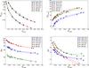 |
Fig. 1 Comparison of the grid quality metrics for octree and k-d-tree based grids of our three test cases (stars correspond to octree grids, dots to k-d tree grids, and the different colours correspond to the three different test models). The top left panel shows Ncells, the total number of cells in the grid, as a function of the threshold mass fraction δmax. For a given threshold value, octree grids require up to more than double the number of cells compared to the corresponding k-d tree. The other panels show the average number of cells crossed per path ⟨ Ncross ⟩, the density quality metric Δρ, and the optical depth quality metric Δτ as a function of Ncells. |
3.3. Results
Figure 1 shows the results of a comparison of octree- and k-d-tree based SKIRT simulations of our three test cases. The top left panel shows Ncells, the total number of cells in the grid, as a function of the threshold mass fraction δmax. Impressively, for a fixed value of δmax, the k-d tree generates only half as many cells as the octree, irrespective of the chosen model. This alone already strongly advocates for the use of k-d trees in radiative transfer simulations.
In the top right panel of Fig. 1 we show the average number of cells crossed per path. If we would have plotted this quantity as a function of the threshold mass fraction δmax, the k-d tree would easily beat the octree grid, as the former contains only half the number of cells of the latter. If we plot ⟨ Ncross ⟩ as a function of Ncells, the picture is more mixed: the k-d tree performs slightly better than the octree for the logarithmic spiral galaxy models, but slightly worse for the other two models. Averaging out, we find that the average straight path through the k-d tree crosses roughly the same number of cells as the average path through the octree with the same total number of cells (with a more relaxed value of δmax).
Looking at the quality of the grids, we find that, for a fixed δmax, the octree grids have a more accurate discretization than the corresponding k-d trees. This is no surprise, as they contain up to double as many cells. On the other hand, if we compare the quality of the octree and k-d tree grids for fixed values of Ncells (bottom panels of Fig. 1), the results turn around: for a fixed number of cells, the k-d tree grids typically correspond to lower values of Δρ and Δτ compared to the octree grids. This means that, for a certain required density or optical depth grid quality, we can generate a k-d tree with roughly 20% fewer cells compared to an octree grid. The general conclusion of this investigation is that the k-d tree based grids outperform the octree grids in all grid quality measures. As they are as simple to implement as the more widely used octree grids, we recommend their use in radiative transfer codes.
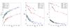 |
Fig. 2 Comparison of the grid quality metrics for octree (stars) and k-d-tree (dots) based grids of the spiral galaxy model, using different node subdivision stopping criteria. The blue lines correspond to a mass threshold only, the red lines lines to an optical depth threshold only, and the green lines to a combination of both criteria. The different panels represent the average number of cells crossed per path ⟨ Ncross ⟩, the density quality Δρ, and the optical depth quality metric Δτ as a function of the total number of cells in the grid, Ncells. |
4. Subdivision stopping criteria for hierarchical tree construction
4.1. Dust mass and optical depth criteria
Ideally, the spatial dust grid used in radiative transfer simulations should be optimized to discretize the intensity of the radiation field, the fundamental quantity that is the objective of radiative transfer studies. Obviously, this quantity is not known at the beginning of a radiative transfer simulation, which makes the task to set up the grid hard: the challenge is to construct the best possible grid without a priori knowledge of the radiation field. The most obvious choice is to base the grid on the dust density field, but the question still remains on which criterion we should base the discretization.
For the construction of both the octree and the k-d tree based dust grids we have used so far, we have adopted a simple mass-based criterion to stop the recursive subdivision of the nodes. As long as the fractional dust mass δ = M/Mtot in a node is larger than a preset threshold value δmax, the node is further subdivided. Here, the mass in a node is determined by evaluating the true input density at Nran randomly generated positions xi within the node, i.e. 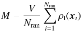 (1)with V the volume of the node. This criterion ensures that there will be more subdivision, and hence higher resolution, in regions with higher density, which is exactly what is desired. Moreover, the criterion is very easy to implement. One weakness of this construction algorithm is that does not distinguish between large cells with a low dust density and small cells with a large density. This implies that different cells, even if they contain the same dust mass, can have strongly different volumes or densities. In order to resolve the crucial regions where the radiation field changes most rapidly, it probably makes sense to subdivide those cells with a high density slightly more than the ones with a lower density, even if they contain the same mass. This inspired us to look for another criterion that can be used instead of, or in addition to, the mass criterion.
There are different possible options that can be explored to stimulate the subdivision of nodes with a high density. All of these, essentially, use a combination of the mass and the volume of a node, and these quantities are easy to calculate during the construction of the tree. We have opted for an optical depth criterion, where we continue the subdivision if the optical depth of a node is larger than a threshold τmax. For the optical depth of a node, we use the maximum optical depth through the node. For cuboidal nodes (as we have in our octree and k-d tree grids), with sides a, b and c, total mass M and opacity κ, the optical depth is 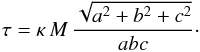 (2)We prefer this criterion above, for example, a criterion based on the mean density, as the optical depth is a quantity that has a direct link to the radiative problem (changes in the radiation field are proportional to the optical depth in the optically thin cases).
A first question to consider is whether this optical depth criterion can be used an alternative for the mass criterion we have used so far. In Fig. 2 we show the results of test simulations based on the logarithmic three-armed spiral galaxy model. For both the octree grid (stars) and the k-d tree grid (dots), we constructed a set of dust grids using only a mass criterion (blue lines) and using only an optical depth criterion (red lines). The three different panels compare the grid metrics ⟨ Ncross ⟩, Δρ and Δτ as a function of the total number of grid cells Ncells. It is clear from this figure that using only the optical depth criterion is not a sensible option. For a fixed Ncells, an optical depth based grid has a stronger subdivision in the high density regions compared to a grid with mass based subdivision, but, unavoidably, this also results in a larger number of large cells. The positive result is that the former grids are faster, in the sense that the average path crosses fewer cells. However, this advantage does not weigh up against the loss of accuracy: the optical depth based grids have a much poorer accuracy than the mass based grids, as measured by both Δρ and Δτ. To achieve the same accuracy, around an order of magnitude more cells are required.
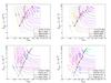 |
Fig. 3 Contour plots illustrating different properties of octree grids (left panels) and k-d tree grids (right panels), corresponding as a function of the δmax and τmax threshold values. The solid lines in each panel correspond to lines of equal numbers of grid cells, whereas the dashed lines correspond to iso-quality contours, corresponding to the density quality metric Δρ (top panels) and the optical depth quality metric Δτ (bottom panel). |
This does not imply that the optical depth criterion is useless, as it can also be combined with the mass criterion. In Fig. 2 we also show the results of a grid that uses a combination (green lines) of both criteria (details on how these two criteria are combined are given below). Here we clearly see that the combination is advantageous: by combining both criteria, we can improve the accuracy of the grid, as measured by both Δρ and Δτ, and we decrease the average number of cells crossed on a path, resulting in a speed-up of the simulation.
A useful tool to understand the complex interplay between these two quantities are contour plots that display the total number of grid cells and the different grid quality metrics as a function of the stopping criteria τmax and δmax. Figure 3 shows such plots for the logarithmic three-armed spiral galaxy model, for both the octree and k-d tree grids. In each of these panels, the stopping criteria become more stringent towards the bottom-left corner. Consequently, the number of cells and the quality increase towards that same corner.
From these plots, we can identify the best combination of the stopping criteria to construct a grid with a certain quality metric. Assume, for example, that we want to construct an octree based grid with a density quality metric Δρ = 375 (recall that the absolute value is not relevant). We can then look at the top left plot, which displays the contours of Ncells and Δρ as a function of δmax and τmax. The contour corresponding to Δρ = 375 connects all points in the parameters space that correspond to grids with the same quality. We can, for example, create such a grid by setting δmax = 3 × 10⁻⁶ and τmax = 0.033, and looking at the Ncells contours, we see that this grid will contain about 1.2 million grid cells. We can relax the mass criterion to δmax = 6 × 10⁻⁶ and tighten the optical depth criterion to τmax = 0.026: this will yield a grid with the same density quality, but the number of grid cells reduces to about 1 million. If we relax the mass threshold even further to δmax = 10-5 and tighten the optical depth threshold to τmax = 0.022, we obtain another grid with the same density quality, but the number of cells increases again to about 1.4 million. The same exercise can be repeated for other values of the density quality, but also for the optical depth quality. The bottom-line is always the same: for a given quality requirement, there seems to be an optimal combination of δmax and τmax that yields grids with a minimum number of cells. Typically, the number of cells in this ideal combination is reduced by 20% compared to the grid based on a mass criterion only (which corresponds to the asymptotic values of the contours towards the right in the panels of Fig. 3).
These figures also demonstrate the superiority of the k-d tree compared to the octree, also in the case when more advanced tree construction criteria are adopted. Taking the same example as used above, we see that the smallest octree with a density quality Δρ = 375 contains around 1 million cells, whereas a k-d tree with 800 000 cells can be constructed with the same quality.
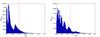 |
Fig. 4 Histograms of the distribution of the optical depth τcell in each cell for the spiral galaxy model octree grid (left panel) and k-d tree (right panel), corresponding to a mass threshold criterion δmax = 3 × 10⁻⁶. |
The question is now how the two criteria need to be combined to give the optimal results. In other words, how do we set the values δmax and τmax such that this combination is ideal? In our parameter space study, we can identify these point by searching along every iso-quality contour the point that corresponds to the smallest number of grid cells. These points are indicated in red in the different panels of Fig. 3. However, it is obviously impossible to construct this entire parameter space of grids for every possible radiative transfer simulation. Instead, it would be useful to have a simple recipe that can identify this combination. A simple numerical relation between δmax and τmax seems impossible, as the useful range of τmax values depends on the total mass, the geometric complexity, and the opacity of our model.
Our approach consists of two steps. As a first step, we fix the value of δmax and construct a grid using this subdivision stopping criterion only. Subsequently, we look at the distribution of the optical depth of the cells. Fig. 4 shows the histograms of cell optical depth for the logarithmic spiral galaxy models for a fixed δmax = 3 × 10⁻⁶, for the octree and k-d tree grids respectively. In both histograms, there is a long tail of high optical depth, but not necessarily high mass, cells which are the prime candidates for further subdivision. The vertical lines in these plots indicates the 90% percent of the optical depth distribution, which we found to be a suitable value as to where this distribution should be cut off. In order words, we create an ordered list of the τ values, and we set τmax equal to the optical depth of the cell at position 0.9 Ncells. The combinations of δmax and τmax we have obtained in this way are indicated as green dots in the different panels of Fig. 3, and they lie very close to the optimal points recovered from searching the parameter space.
This recipe of finding the optimal value of τmax corresponding to a given value of δmax is simple and fast, as the necessary calculations are easily done during the tree construction phase. The recipe is exactly the same for both octree and k-d tree based grids. Our conclusion is that an additional optical depth criterion, chosen according to a simple recipe, is very useful in producing octree or k-d trees with fewer cells for a given quality requirement, or vice versa, with higher quality for a fixed number of grid cells.
4.2. Strong gradients and sharp edges
The other problem we referred to in the Introduction is the issue of very strong gradients or sharp boundaries in the density fields. Grids based on a mass criterion (or the combination of a mass and optical depth criterion) have difficulties in dealing with these. A clear example is the octree based grid for the clumpy AGN model considered by Saftly et al. (2013). This model is characterized by a density field with sharp boundaries at the edges of the torus. During the tree construction process, we encounter many nodes at the edges of this boundary, that only have a tiny and compact corner filled with dust. When we compute the dust mass in such a node, it will soon be below the dust mass (and/or optical depth) threshold, such that the subdivision is stopped. This result is relatively large cells with a relatively low density, whereas the true underlying density field is relatively high in one tiny corner and zero in most of the cell, see the central panel in Fig. 6. This automatic stopping of subdivision is a problem, as the regions with strong density gradients and/or sharp boundaries are exactly regions that we want to resolve at high resolution.
One way to solve this problem is to introduce artificial boundaries in the grid. In the case of the clumpy AGN model, one could construct a hierarchical grid within the sharp boundaries of the torus itself. This solution might work efficiently for a number of analytical models, but it is not the general solution desired for arbitrary applications, where the occurrence and location of sharp boundaries and strong gradients is not always known a priori.
Our proposed solution is to introduce a node subdivision criterion that depends on the density gradient within a node, and add this criterion to the already applied dust mass (and optical depth) threshold criteria. We have considered a very simple approach that does not introduce a strong computational overhead. During the construction of the grid, the mass density is evaluated in Nran random positions in each node as part of the estimate of the mass in that node. If a certain node is not to be subdivided further according to the δmax and/or τmax criteria, we compute the quantity 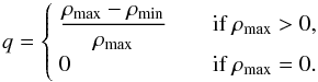 (3)where ρmin and ρmax are the smallest and largest sampled density values from the list of Nran sampled positions in the node. This quantity is a simple measure for the uniformity of the density within the node: for a constant density in the node, q = 0, whereas q approaches 1 if a steep gradient is present. The additional criterion we impose is that a node is subdivided if q exceeds a preset maximum value qmax ≲ 1. In principle, nodes that contain a sharp edge will continue to be subdivided for ever, since such cells have by definition q = 1. Thus it is important to always specify a reasonable maximum subdivision level when using this subdivision criterion.
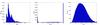 |
Fig. 5 Histograms of the distribution of the density dispersion q in each cell in our three models using the k-d tree grids, corresponding to a mass threshold criterion δmax = 3 × 10⁻⁶. The left panel is the three-armed spiral galaxy model, the middle panel the clumpy AGN model, and the right panel the SPH galaxy model. |
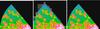 |
Fig. 6 Illustration on how the density dispersion criterion qmax solves the problem of sharp edges in models such as the AGN torus. In this example we used an octree grid. The left panel represents a cut through the true dust density in xz plane, and the central panel shows the grid density as obtained without a density dispersion criterion with about 3 million cells. The edges of the torus are clearly poorly resolved. The right panel shows the grid density after adding the density dispersion criterion qmax = 0.99 and a maximum subdivision level of 10. The edges are now extremely well resolved using about 7 million of additional cells. |
In Fig. 5 we show histograms of q for k-d tree based grids for the three test models we consider, before applying any q-based subdivision. The logarithmic three-armed spiral galaxy model (left panel) is the smoothest and most regular of the three models, and is characterized by cells in which the vast majority has q < 0.35. The SPH galaxy model (right panel) is characterized by a somewhat more irregular, but still relatively smooth density field. The corresponding distribution of q values is a fairly broad distribution that peaks around 0.35 and then decreases smoothly towards larger values of q. A small number of cells have q = 1: these correspond to cells at the edges of cavities in the dust density. Finally, the clumpy AGN model (central panel) is designed to be a test model with strong density gradients and sharp edges. This is clearly evident in the histogram: a large fraction of the cells is characterized by large values of q and particularly conspicuous is the large number of cells with q = 1, corresponding to grid cells overlapping with the sharp edge of the torus. In such a model, we clearly need higher resolution for those cells. Figure 6 illustrates the differences in the octree based grid for this model before and after adding the q-based subdivision criterion. This simple recipe clearly solves the problem.
5. Discussion and conclusion
The main goal of this paper was to critically investigate the efficiency and accuracy of the standard octree algorithm in the context of radiative transfer simulations, and to investigate the use of alternative hierarchical grid structures and node subdivision stopping criteria beyond a straightforward mass threshold value.
We have investigated the use of hierarchical k-d tree grids as an alternative to octree grids to partition the transfer medium. We have implemented a flexible k-d tree structure in the 3D Monte Carlo code SKIRT (Baes et al. 2003, 2011). The construction algorithm of the k-d tree is completely similar to the technique we used for the construction of the octree grid in SKIRT, and we can use the same, very efficient, neighbour list search grid traversal method. Using three different test models, and a set of objective grid quality metrics, we have critically compared the octree and k-d based grids. We have found that, for a fixed value of the mass threshold δmax, the k-d tree generates only half as many cells as the octree, irrespective of the chosen model. Moreover, if we compare the quality of the octree and k-d tree grids for a fixed total number of cells, the latter have a higher accuracy. We can generate a k-d tree with roughly 20% fewer cells compared to an octree grid for a certain required density or optical depth quality.
As a second objective, we have investigated whether there are useful alternatives to the simple mass threshold as a criterion to stop the recursive subdivision of the nodes in hierarchical trees (both octrees and k-d trees). In order to stimulate the subdivision of small, high-density cells, we have tested the option of an optical depth criterion, but this gave rise to grids with an unacceptably low accuracy. A combination of a mass and an optical depth criterion, however, turned out to be a sensible criterion. Using an optimal combination of both, it was possible to reduce the number of cells in the grids by 20% for a given quality requirement, and also decrease the average number of cells crossed on a path, resulting in faster run time of the simulations. We have presented a simple recipe that enables us to approximate this optimal combination without the need to scan the entire parameter space.
Finally, we have considered the problem caused by discontinuities, strong gradients or sharp edges. In hierarchical grids (octrees or k-d trees) governed by mass and/or optical depth threshold criteria, such features can lead to undesirable large, low-density cells, whereas a strong subdivision is particularly needed in these cases. We have presented a simple solution for this problem, in the form of an additional gradient threshold criterion. The criterion is very simple to implement and is shown to give the desired results.
The main results of this investigation are that, in the context of radiative transfer simulations, we can strongly advocate the use of the lesser-known k-d trees as an alternative to the popular octrees, and that the combination of different subdivision stopping criteria, rather than a simple mass criterion, can lead to more efficient grids. While this is another step forward towards the construction of the ideal grid, we are well aware that this is not the end stage. A number of side notes are required.
The first caveat refers to the different grid quality metrics that we have used in this paper. We have attempted to quantify the quality of a grid using different criteria: the total number of cells, the average number of cells crossed per path, and an estimate of the standard deviation of the density and optical depth discretization error. These quantities are an attempt to translate what one would consider intuitively as a good grid to a quantitative measure by which different grids can be compared. They are only based on the dust density field, and they are relatively straightforward to calculate. But the question remains whether these metrics are sufficient to really measure whether one grid is better than the other for radiative transfer simulations. The ideal spatial grid in radiative transfer simulations should discretize the intensity of the radiation field as accurately as possible, but this quantity is unknown at the start of the simulation (it is exactly the goal of radiative transfer simulation to recover the radiation field). As the radiation field is not only determined by the dust density, but equally well by the distribution of sources and the optical properties of the dust, it is simply impossible to construct the ideal grid with only knowledge of the dust density field, or to construct grid quality metrics based on the density field alone that measure the appropriateness neighbour of a grid. As suggested by Saftly et al. (2013), a more advanced option could in principle be achieved iteratively from running a series of radiative transfer simulations, in which the grid is adapted at every step based on the properties of the radiation field (strength of the radiation field, temperature distribution, ...) in the previous iteration step (see also Niccolini & Alcolea 2006). This approach is clearly too complex and time-consuming for every single simulation. Grid construction guidelines and quality metrics based on the dust density field alone, such as discussed in this paper, are probably a good compromise between effectiveness and computational cost, but future work might investigate this in more detail.
The second side note is that the grids we have considered here constitute only a small corner of the entire zoo of possible grid structures that could be considered. Octrees and k-d trees are only two members of the large family of hierarchical grids that have been developed as space partitioning structures. In the field of computational geometry and computer graphics, a wider range of space partitioning structures are used for different goals, and hierarchical AMR grids (or the so-called grids-in-grids) are also used in several radiative transfer codes (e.g. Wolf 2003; Tasitsiomi 2006; Laursen et al. 2009; Robitaille 2011; Heymann & Siebenmorgen 2012; Lunttila & Juvela 2012). Havran (2000) did an extensive comparison of heuristic ray-shooting algorithms based on many different space partitioning structures (BSP trees, k-d trees, octrees, bounding volume hierarchies, uniform grids, and three types of hierarchical grids) and found that the ray-shooting algorithm based on the k-d tree is the winning candidate among all tested algorithms. This gives us some confidence that, among the class of hierarchical grids, the k-d tree is an ideal candidate for radiative transfer grids, but other candidates might have their own advantages.
The same might also be true for unstructured grids, which belong to a different section of the family of space partitioning structures. Particularly interesting are unstructured grids based on Voronoi or Delaunay tessellation. These grids have existed for a long time, but they have recently gained increases popularity thanks to the development of hydrodynamics codes that operate on them (Xu 1997; Springel 2010; Duffell & MacFadyen 2011). Radiative transfer on such grids has been shown to be possible (Paardekooper et al. 2010; Brinch & Hogerheijde 2010; Camps et al. 2013). While unstructured grids can probably not compete with hierarchical grids in terms of grid traversal, they could be more efficient in some situations, e.g. in simulations where in-cell operations (such as the calculation of the temperature distribution or the dust emission profile), rather than grid traversal, are the most expensive operation.
Acknowledgments
W.S. acknowledges the support of Al-Baath University and The Ministry of High Education in Syria in the form of a research grant. This work fits in the CHARM framework (Contemporary physical challenges in Heliospheric and AstRophysical Models), a phase VII Interuniversity Attraction Pole (IAP) programme organised by BELSPO, the BELgian federal Science Policy Office.
References
- Baes, M., Davies, J. I., Dejonghe, H., et al. 2003, MNRAS, 343, 1081 [NASA ADS] [CrossRef] [Google Scholar]
- Baes, M., Verstappen, J., De Looze, I., et al. 2011, ApJS, 196, 22 [NASA ADS] [CrossRef] [Google Scholar]
- Bentley, J. L. 1975, Commun. ACM, 18, 509 [CrossRef] [Google Scholar]
- Bianchi, S. 2008, A&A, 490, 461 [NASA ADS] [CrossRef] [EDP Sciences] [Google Scholar]
- Brinch, C., & Hogerheijde, M. R. 2010, A&A, 523, A25 [NASA ADS] [CrossRef] [EDP Sciences] [Google Scholar]
- Camps, P., Baes, M., & Saftly, W. 2013, A&A, 560, A35 [NASA ADS] [CrossRef] [EDP Sciences] [Google Scholar]
- Duffell, P. C., & MacFadyen, A. I. 2011, ApJS, 197, 15 [NASA ADS] [CrossRef] [Google Scholar]
- Fuchs, H., Kedem, Z. M., & Naylor, B. 1979, SIGGRAPH Comput. Graph., 13, 175 [CrossRef] [Google Scholar]
- Fuchs, H., Kedem, Z. M., & Naylor, B. F. 1980, SIGGRAPH Comput. Graph., 14, 124 [CrossRef] [Google Scholar]
- Glassner, A. S. 1984, IEEE Comput. Graph. Appl., 4, 15 [Google Scholar]
- Gordon, K. D., Misselt, K. A., Witt, A. N., & Clayton, G. C. 2001, ApJ, 551, 269 [NASA ADS] [CrossRef] [Google Scholar]
- Harries, T. J., Monnier, J. D., Symington, N. H., & Kurosawa, R. 2004, MNRAS, 350, 565 [NASA ADS] [CrossRef] [Google Scholar]
- Havran, V. 2000, Ph.D. Thesis, Czech Technical University [Google Scholar]
- Heymann, F., & Siebenmorgen, R. 2012, ApJ, 751, 27 [NASA ADS] [CrossRef] [Google Scholar]
- Jonsson, P. 2006, MNRAS, 372, 2 [NASA ADS] [CrossRef] [Google Scholar]
- Kurosawa, R., & Hillier, D. J. 2001, A&A, 379, 336 [NASA ADS] [CrossRef] [EDP Sciences] [Google Scholar]
- Laursen, P., Razoumov, A. O., & Sommer-Larsen, J. 2009, ApJ, 696, 853 [Google Scholar]
- Lunttila, T., & Juvela, M. 2012, A&A, 544, A52 [NASA ADS] [CrossRef] [EDP Sciences] [Google Scholar]
- MacDonald, D. J., & Booth, K. S. 1990, Vis. Comput., 6, 153 [CrossRef] [Google Scholar]
- Misiriotis, A., Kylafis, N. D., Papamastorakis, J., & Xilouris, E. M. 2000, A&A, 353, 117 [NASA ADS] [Google Scholar]
- Niccolini, G., & Alcolea, J. 2006, A&A, 456, 1 [NASA ADS] [CrossRef] [EDP Sciences] [Google Scholar]
- Paardekooper, J.-P., Kruip, C. J. H., & Icke, V. 2010, A&A, 515, A79 [NASA ADS] [CrossRef] [EDP Sciences] [Google Scholar]
- Pinte, C., Ménard, F., Duchêne, G., & Bastien, P. 2006, A&A, 459, 797 [NASA ADS] [CrossRef] [EDP Sciences] [Google Scholar]
- Rahimi, A., & Kawata, D. 2012, MNRAS, 422, 2609 [NASA ADS] [CrossRef] [Google Scholar]
- Reshetov, A., Soupikov, A., & Hurley, J. 2005, ACM Trans. Graph., 24, 1176 [CrossRef] [Google Scholar]
- Robitaille, T. P. 2011, A&A, 536, A79 [NASA ADS] [CrossRef] [EDP Sciences] [Google Scholar]
- Saftly, W., Camps, P., Baes, M., et al. 2013, A&A, 554, A10 [NASA ADS] [CrossRef] [EDP Sciences] [Google Scholar]
- Schechtman-Rook, A., Bershady, M. A., & Wood, K. 2012, ApJ, 746, 70 [NASA ADS] [CrossRef] [Google Scholar]
- Shevtsov, M., Soupikov, A., & Kapustin, A. 2007, Comput. Graph. Forum, 26, 395 [CrossRef] [Google Scholar]
- Springel, V. 2010, MNRAS, 401, 791 [NASA ADS] [CrossRef] [Google Scholar]
- Stalevski, M., Fritz, J., Baes, M., Nakos, T., & Popović, L. Č. 2012, MNRAS, 420, 2756 [NASA ADS] [CrossRef] [Google Scholar]
- Steinacker, J., Bacmann, A., & Henning, T. 2006, ApJ, 645, 920 [NASA ADS] [CrossRef] [Google Scholar]
- Steinacker, J., Baes, M., & Gordon, K. D. 2013, ARA&A, 51, 63 [NASA ADS] [CrossRef] [Google Scholar]
- Tasitsiomi, A. 2006, ApJ, 645, 792 [NASA ADS] [CrossRef] [Google Scholar]
- Wald, I., & Havran, V. 2006, in IEEE Symp. on Interactive Ray Tracing, 61 [Google Scholar]
- Whitney, B. A. 2011, BASI, 39, 101 [Google Scholar]
- Whitney, B. A., Robitaille, T. P., Bjorkman, J. E., et al. 2013, ApJS, 207, 30 [NASA ADS] [CrossRef] [Google Scholar]
- Wolf, S. 2003, Comput. Phys. Commun., 150, 99 [NASA ADS] [CrossRef] [Google Scholar]
- Xilouris, E. M., Kylafis, N. D., Papamastorakis, J., Paleologou, E. V., & Haerendel, G. 1997, A&A, 325, 135 [NASA ADS] [Google Scholar]
- Xu, G. 1997, MNRAS, 288, 903 [NASA ADS] [CrossRef] [Google Scholar]
- Zhou, K., Hou, Q., Wang, R., & Guo, B. 2008, ACM Trans. Graph., 27, 126 [Google Scholar]
All Figures
|
Fig. 1 Comparison of the grid quality metrics for octree and k-d-tree based grids of our three test cases (stars correspond to octree grids, dots to k-d tree grids, and the different colours correspond to the three different test models). The top left panel shows Ncells, the total number of cells in the grid, as a function of the threshold mass fraction δmax. For a given threshold value, octree grids require up to more than double the number of cells compared to the corresponding k-d tree. The other panels show the average number of cells crossed per path ⟨ Ncross ⟩, the density quality metric Δρ, and the optical depth quality metric Δτ as a function of Ncells. |
| In the text | |
|
Fig. 2 Comparison of the grid quality metrics for octree (stars) and k-d-tree (dots) based grids of the spiral galaxy model, using different node subdivision stopping criteria. The blue lines correspond to a mass threshold only, the red lines lines to an optical depth threshold only, and the green lines to a combination of both criteria. The different panels represent the average number of cells crossed per path ⟨ Ncross ⟩, the density quality Δρ, and the optical depth quality metric Δτ as a function of the total number of cells in the grid, Ncells. |
| In the text | |
|
Fig. 3 Contour plots illustrating different properties of octree grids (left panels) and k-d tree grids (right panels), corresponding as a function of the δmax and τmax threshold values. The solid lines in each panel correspond to lines of equal numbers of grid cells, whereas the dashed lines correspond to iso-quality contours, corresponding to the density quality metric Δρ (top panels) and the optical depth quality metric Δτ (bottom panel). |
| In the text | |
|
Fig. 4 Histograms of the distribution of the optical depth τcell in each cell for the spiral galaxy model octree grid (left panel) and k-d tree (right panel), corresponding to a mass threshold criterion δmax = 3 × 10⁻⁶. |
| In the text | |
|
Fig. 5 Histograms of the distribution of the density dispersion q in each cell in our three models using the k-d tree grids, corresponding to a mass threshold criterion δmax = 3 × 10⁻⁶. The left panel is the three-armed spiral galaxy model, the middle panel the clumpy AGN model, and the right panel the SPH galaxy model. |
| In the text | |
|
Fig. 6 Illustration on how the density dispersion criterion qmax solves the problem of sharp edges in models such as the AGN torus. In this example we used an octree grid. The left panel represents a cut through the true dust density in xz plane, and the central panel shows the grid density as obtained without a density dispersion criterion with about 3 million cells. The edges of the torus are clearly poorly resolved. The right panel shows the grid density after adding the density dispersion criterion qmax = 0.99 and a maximum subdivision level of 10. The edges are now extremely well resolved using about 7 million of additional cells. |
| In the text | |
Current usage metrics show cumulative count of Article Views (full-text article views including HTML views, PDF and ePub downloads, according to the available data) and Abstracts Views on Vision4Press platform.
Data correspond to usage on the plateform after 2015. The current usage metrics is available 48-96 hours after online publication and is updated daily on week days.
Initial download of the metrics may take a while.