| Issue |
A&A
Volume 561, January 2014
|
|
|---|---|---|
| Article Number | A120 | |
| Number of page(s) | 12 | |
| Section | Interstellar and circumstellar matter | |
| DOI | https://doi.org/10.1051/0004-6361/201322347 | |
| Published online | 21 January 2014 | |
The CHESS survey of the L1157-B1 bow-shock: high and low excitation water vapor⋆
1 INAF – Istituto di Astrofisica e Planetologia Spaziali, via del Fosso del Cavaliere 100, 00133 Roma, Italy
e-mail: This email address is being protected from spambots. You need JavaScript enabled to view it.
2 UJF-Grenoble 1/CNRS-INSU, Institut de Planétologie et d’Astrophysique de Grenoble (IPAG) UMR 5274, 38041 Grenoble, France
3 Centro de Astrobiologia, CSIC-INTA, Carretera de Torrejón a Ajalvir, km 4, Torrejón de Ardoz, 28850 Madrid, Spain
4 INAF – Osservatorio Astrofisico di Arcetri, Largo Enrico Fermi 5, 50125 Firenze, Italy
5 Observatoire de Paris, LERMA, UMR 8112 du CNRS, ENS, UPMC, UCP, 61 Av. de l’Observatoire, 75014 Paris, France
6 INAF – Osservatorio Astronomico di Roma, via di Frascati 33, 00040 Monte Porzio Catone, Italy
7 Department of Physics and Astronomy, University College London, Gower Street, London WC1E 6BT, UK
8 LERMA, UMR 8112 du CNRS, Observatoire de Paris, École Normale Supérieure, 24 rue Lhomond, 75231 Paris Cedex 05, France
Received: 23 July 2013
Accepted: 12 November 2013
Abstract
Context. Molecular outflows powered by young protostars strongly affect the kinematics and chemistry of the natal molecular cloud through strong shocks. This results in substantial modifications of the abundance of several species. In particular, water is a powerful tracer of shocked material because of its sensitivity to both physical conditions and chemical processes.
Aims. As part of the Chemical HErschel Surveys of Star-forming regions (CHESS) guaranteed time key program, we aim at investigating the physical and chemical conditions of H2O in the brightest shock region B1 of the L1157 molecular outflow.
Methods. We observed several ortho- and para-H2O transitions using the HIFI and PACS instruments on board Herschel toward L1157-B1, providing a detailed picture of the kinematics and spatial distribution of the gas. We performed a large velocity gradient (LVG) analysis to derive the physical conditions of H2O shocked material, and ultimately obtain its abundance.
Results. We detected 13 H2O lines with both instruments probing a wide range of excitation conditions. This is the largest data set of water lines observed in a protostellar shock and it provides both the kinematics and the spatial information of the emitting gas. The PACS maps reveal that H2O traces weak and extended emission associated with the outflow identified also with HIFI in the o-H2O line at 556.9 GHz, and a compact (~10′′) bright, higher excitation region. The LVG analysis of H2O lines in the bow-shock show the presence of two gas components with different excitation conditions: a warm (Tkin ≃ 200–300 K) and dense (n(H2) ≃ (1–3) × 106 cm-3) component with an assumed extent of 10′′, and a compact (~2′′–5′′) and hot, tenuous (Tkin ≃ 900–1400 K, n(H2) ≃ 103−4 cm-3) gas component that is needed to account for the line fluxes of high Eu transitions. The fractional abundance of the warm and hot H2O gas components is estimated to be (0.7–2) × 10-6 and (1–3) × 10-4, respectively. Finally, we identified an additional component in absorption in the HIFI spectra of H2O lines that connect with the ground state level. This absorption probably arises from the photodesorption of icy mantles of a water-enriched layer at the edges of the cloud, driven by the external UV illumination of the interstellar radiation field.
Key words: stars: formation / ISM: individual objects: L1157-B1 / ISM: molecules / ISM: abundances / ISM: jets and outflows
Based on Herschel HIFI and PACS observations. Herschel is an ESA space observatory with science instruments provided by European-led Principal Investigator consortia and with important participation from NASA.
© ESO, 2014
1. Introduction
Molecular outflows are among the most conspicuous manifestations of a nascent star. These outflows are known to result from the entrainment of circumstellar gas, swept up by the primary jet, where a shock front is generated as a consequence of the supersonic impact of the jet with the natal cloud. Shocks heat, accelerate, and compress the ambient gas material switching on a complex chemistry that leads to an enhancement of the abundance of several species in the so-called chemically active outflows (e.g., Bachiller 1996). The nature and properties of these shocks are still not well understood, in particular the role of the magnetic field. Water is predicted to be one of the main gas cooling agents in magnetized shocks, along with H2 and CO (e.g., Draine et al. 1983; Kaufman & Neufeld 1996; Flower & Pineau des Forêts 2010). Thanks to its rich emission spectrum, transitions spanning a wide range of excitation conditions, and its sensitivity to local conditions (e.g., Bergin et al. 1998; van Dishoeck et al. 2011), H2O constitutes a powerful probe of the physics and chemistry of the shock outflow interaction. In particular, in shocked regions H2O abundance can increase by several orders of magnitude, up to ~10-4, through sputtering of grains mantles and formation in the gas phase at high temperatures (Hollenbach & McKee 1989; Kaufman & Neufeld 1996; Flower & Pineau des Forêts 2010).
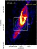 |
Fig. 1 Southern blueshifted outflow lobe observed in CO (1–0) with the Plateau de Bure Interferometer (PdBI) by Gueth et al. (1996). The black cross marks the nominal position of the bow-shock L1157-B1 while the white × symbol indicates the nominal position of the B2 shock (Bachiller & Pérez Gutiérrez 1997). The largest (~38′′) and smallest (~12 |

The outflow powered by the low-mass Class 0 protostar L1157-mm (d ≃ 250 pc; Looney et al. 2007) displays a rich specific chemistry that makes it the prototype of chemically active outflows (e.g., Bachiller & Pérez Gutiérrez 1997; Bachiller et al. 2001; Arce et al. 2008). As such, it is an excellent laboratory for investigating the physical conditions and the formation routes of H2O and its role in the cooling of a typical protostellar outflow. The L1157 outflow has been studied in detail for more than two decades through many molecular lines and in a wide range of wavelengths, from the near infrared (near-IR; e.g., Davis & Eisloeffel 1995; Neufeld et al. 2009; Nisini et al. 2010b) to the radio domain (e.g., Zhang et al. 2000; Bachiller et al. 2001; Tafalla & Bachiller 1995). Several compact shocked regions are found along both the blue- and redshifted lobes (see e.g., Gueth et al. 1998; Nisini et al. 2007, 2010b). In particular, the southern blueshifted lobe, shown in Fig. 1, consists of two limb-brightened cavities, each of which is associated with a bow-shock, probably created by episodic events in a precessing jet (Gueth et al. 1996).
Water emission in L1157-B1 was first detected with the Infrared Space Observatory (ISO) by Giannini et al. (2001); however, only three lines were detected and the physical conditions of H2O could not be constrained. Later on, Odin and the Submillimeter Wave Astronomy Satelilte (SWAS) observed the fundamental o-H2O line emission in the direction of the southern blueshifted lobe of the outflow (Bjerkeli et al. 2009; Franklin et al. 2008). The low angular resolution gave access only to properties averaged over the entire outflow lobe. Assuming that both the H2O and the low-J CO line emission originate in the same gas, these authors inferred an o-H2O abundance ranging between 10-6 and 2 × 10⁻⁴. As part of the Water In Star-forming regions with Herschel (WISH) key program, Nisini et al. (2010a) used PACS to map the o-H2O 179 μm line over the entire outflow structure. These authors detected extended emission, with several strong peaks associated with shocked knots, well spatially correlated with H2 rotational lines (Nisini et al. 2010b).
The molecular bright shock region B1, in the southern lobe of the outflow (see Fig. 1), was selected as one of the targets of the key program Chemical HErschel Surveys of Star-forming regions (CHESS1) dedicated to unbiased spectral line surveys of prototypical star-forming regions (Ceccarelli et al. 2010) in the guaranteed time of the Herschel Space Observatory (Pilbratt et al. 2010).
The CHESS survey of L1157-B1 offers a comprehensive view on the water line emission in a typical protostellar bow-shock, considered the benchmark for shock models (Gusdorf et al. 2008a,b; Flower & Pineau des Forêts 2010, 2012). A grand total of 13 water lines (both ortho and para) have been detected across the submillimeter and far-infrared window with the PACS spectro-imager (Poglitsch et al. 2010) and the HIFI heterodyne instrument (de Graauw et al. 2010), the largest data set of water lines detected so far in a protostellar shock. Both instruments provide us with a detailed picture of the kinematics and the spatial distribution of the water emission in L1157-B1, allowing us to derive strong constraints on the water abundance and the physical conditions in the emitting gas. The layout of the paper is as follows. In Sect. 2 we summarize our observations. In Sect. 3 we present the main results of HIFI and PACS and in Sect. 4 we analyze the excitation conditions of H2O using a large velocity gradient (LVG) model and discuss the origin of the water emission in L1157-B1, presenting, for the first time, a detailed picture of the bow-shock structure through Herschel observations of water lines. Finally, in Sect. 5 we list the main conclusions.
2. Observations and data reduction
2.1. HIFI observations
The HIFI observations were performed in double beam switching mode during 2010 towards the nominal position of B1:  ,
,  . Both polarizations (H and V) were observed simultaneously. The receiver was tuned in double sideband (DSB). Most of the submillimeter window was covered in an unbiased way with HIFI, and the observations were carried out in spectral scanning mode. In order to study the properties of the H2O gas in the high-velocity wings of the outflow, a few lines were observed in pointed mode in order to reach an excellent signal-to-noise ratio (S/N).
We used the wide band spectrometer (WBS), which provides a frequency resolution of 0.5 MHz (i.e., velocity resolution between 0.1 kms-1 and 0.4 kms-1, depending on the wavelength). The data were processed with the ESA supported package Herschel interactive processing environment2 (HIPE, Ott 2010) version 6. Then level 2 fits files were exported and transformed into the GILDAS3 format for baseline subtraction and subsequent sideband deconvolution, which was performed manually. The relative calibration between both receivers (H and V) was found to be very good, and both signals were co-added to improve the noise rms of the data.
The spectral resolution was then degraded to a common velocity resolution of 1 kms-1 in the final single side band (SSB) data set. Uncertainty in the flux calibration was estimated to be ~20%. In Table 1 we summarize the observational parameters of the H2O transitions detected with HIFI (frequency, wavelength, and upper level energy). The main-beam intensity, peak velocity, and the integrated intensity for each transition are also reported. Intensities are expressed in units of main-beam brightness temperature. The telescope parameters (half power beamwidth (HPBW) and main-beam efficiency (ηmb)) are taken from Roelfsema et al. (2012).
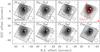 |
Fig. 2 PACS maps of H2O line fluxes (increasing upper-level energy from top left to bottom right). First contour corresponds to the 1σ flux level of each transition. The contour step is 2σ in all lines except for the o-H2O (212 − 101) and o-H2O (303 − 212), for which the contour step is 6σ and 3σ, respectively, where σ is listed in Table 2. The top right panel shows an overlay of the o-H2O (212 − 101) map (gray scale) with the PdBI CH3CN (8–7) K = 0–2 image (red contours) from Codella et al. (2009) tracing the bow-shock. The synthesized beam of PdBI, |


2.2. PACS observations
The PACS observations were carried out on May 25, 2010 in line spectroscopy mode in order to obtain a full-range spectrum of the molecular line emission towards B1, from 55–95.2 μm and from 101.2–210 μm. The spectral scan was centered at the nominal position of B1 (see above) and produced a single 5 × 5 spectral map of  square spatial pixels (hereafter spaxels) over a 47′′ × 47′′ field of view. Two observations were conducted for the 161.5–190.2 μm range. Both measurements are in good agreement, with a discrepancy of at the most ~10%. The resolving power ranges from 1000 to 4000 (i.e., spectral resolution of ~75–300 kms-1) depending on the wavelength, hence water lines are unresolved. The PACS data were processed with HIPE version 5.0. The absolute flux scale was determined from observations of Neptune by normalizing the observed flux to the telescope background, with an estimated uncertainty of ~10% for λ < 190 μm (i.e., where all the water PACS lines lie). Further details of the PACS observations are described in Benedettini et al. (2012), where the emission lines of CO, OH, and the [OI] lines are presented and discussed.
In Table 2 we list the detected transitions, giving their frequency, wavelength, upper energy level, and beam size. We extracted the flux toward each spaxel adopting a Gaussian instrumental response. The line fluxes measured toward the two brightest spaxels, at offsets (0′′, 0′′) and (− 5′′, 7′′), associated with the nominal position of B1 and the high-excitation CO emission peak (Benedettini et al. 2012), respectively, are given in Table 2.
2.3. Cross calibration
Four lines were observed by both PACS and HIFI instruments, which allowed us to check the consistency of the calibration: H2O (212–101) at 179 μm, (221–212) at 180 μm, CO (16–15), and CO (14–13). Using the PACS maps, we estimated the line intensities in the HIFI main-beam solid-angle towards the nominal position of B1. Comparison of the HIFI- and PACS-based line intensities shows a very good agreement for H2O (212 − 101) and CO (14–13), where the integrated intensities are 13.7/14.2 K kms-1 and 5.0/5.5 K kms-1, respectively (for HIFI/PACS instruments), resulting in a discrepancy of ~10%. For the H2O (221 − 212) and CO (16–15) lines, the HIFI/PACS integrated intensities are 2.0/1.8 K kms-1 and 3.4/2.7 K kms-1, respectively. For these lines the discrepancy is larger, about ~20%, but always within the absolute flux calibration uncertainty. We note that both lines are weaker, and the S/N of the data much lower than the other two lines. Overall, we conclude that the agreement between the HIFI and PACS calibration scales is very good.
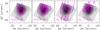 |
Fig. 3 Contour maps of the SiO (2–1) high-velocity (v< − 8 kms-1) emission from Gueth et al. (1998) convolved to the |
3. Results
We have detected 13 H2O transitions with a flux above the 5σ level: 7 H2O transitions (5 ortho, 2 para) in the PACS range (55–210 μm), 8 H2O transitions (5 ortho, 3 para) with HIFI between 672 μm and 180 μm. We note that the 179 μm and 180 μm lines have been detected with both instruments. The o-H2O (321 − 312) transition is detected at a 3σ level with HIFI (see Table 1). Two additional o-H2O transitions (321 − 210 at 75.38 μm and 423 − 414 at 132.41 μm) are tentatively detected with PACS at the 3σ level at the offset position (−5′′, 7′′) (see Table 2). Overall, we detected only transitions of rather low Eu, with values ranging between 26.7 K and 319.5 K.
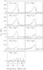 |
Fig. 4 HIFI H2O spectra of L1157-B1 smoothed to a velocity resolution of 1 kms-1. The H2O transition is indicated in each panel. The vertical dashed line marks the ambient LSR velocity vLSR ~ 2.6 kms-1 from C18O emission (Bachiller & Pérez Gutiérrez 1997). |
3.1. H2O spatial distribution
Maps of o-H2O and p-H2O lines observed with PACS are presented in Fig. 2. Water is detected over the entire outflow cavity, both upstream and downstream of the bow-shock; its distribution overlaps rather well with the B1 bow-shock as traced by CH3CN (Codella et al. 2009, see top right panel of Fig. 2) and the outflow walls of the B1 cavity, traced by CO at the PdBI (Gueth et al. 1996, see Fig. 1). Downstream of B1, weak emission is present 20″ away from the shock in several transitions, including the 303 − 212 and 212 − 101 lines, in agreement with Nisini et al. (2010a). This extended emission, which consists of a plateau of low H2O brightness, is related to the ouflow, possibly from the B2 outflow cavity.
Leaving aside the contribution of the plateau to the emission, the distribution of the water emission in B1 displays little variation between the various transitions, with a typical deconvolved size at full-width at half maximum (FWHM) of ~10′′. Overall, the emission appears elongated along the major outflow axis. The H2O brightness peak is located ≈6′′ north of the center of the PACS array, lying approximately halfway between the nominal position of B1 and the high-J CO emission peak identified by Benedettini et al. (2012), at the interface between spaxels (2,2) and (3,2) at offsets (0′′,0′′) and (− 5′′,7′′), respectively. However, size and position determination from the PACS undersampled data are just indicative and they suffer large uncertainties.
It is interesting to compare the morphology of the 212 − 101 line with that of other shock tracers (see Fig. 3). One can see that both H2O and SiO peak at the same position, between offset (0′′,0′′) and (− 5′′,7′′). Similar to H2O, the emission of the mid-IR H2 0–0 S(1) pure-rotational line observed with Spitzer (Nisini et al. 2010b) is extended, partly tracing the B1 cavity, while CO (16–15) and the near-IR H2 1–0 S(1) ro-vibrational line (Caratti o Garatti et al. 2006) are rather compact and peak at offset (− 5′′,7′′), coinciding with the partly dissociative shock driven by the impact of the jet against the B1 cavity (Benedettini et al. 2012). However, it is worth noting that there is also bright H2O emission at the peak of the high-J CO position, suggesting that part of the H2O emission coincides with CO. The good match between SiO (2–1) and H2O (212 − 101), both in terms of spatial distribution and the line profiles in the high-velocity range (see Fig. 2b of Lefloch et al. 2012), provides us with an estimate of the size of the water line emission, ≈10′′, consistent with the PACS determination.
3.2. Line profiles
Figure 4 shows a montage of the water line spectra observed with HIFI smoothed to a velocity resolution of 1 kms-1. Water line profiles are rather broad, with a FWHM ~ 10 kms-1. The bulk of the emission in all transitions is clearly blueshifted with respect to the cloud systemic velocity vLSR = +2.6 kms-1 (Bachiller & Pérez Gutiérrez 1997). For lines with a S/N high enough, e.g., 312–303, 3σ emission is detected at velocities up to − 30 kms-1.
The coexistence of multiple excitation components in L1157-B1 has been studied recently by Lefloch et al. (2012), who showed, based on the spectral slope, that the CO line emission arises from three different emitting regions. These components were tentatively identified as the jet impact shock region (g1), the cavity walls of the L1157-B1 bow-shock (g2), and the cavity walls from the earlier ejection episode that produced the L1157-B2 bow-shock (g3). A schematic view of all these components is presented in Fig. 7. The authors showed that each component is characterized by an specific excitation temperature. We found that the profile of the o-H2O (312 − 303) transition follows the same specific spectral signature observed for the CO (16–15) line profile (see Fig. 2b of Lefloch et al. 2012), which defines the g1 component.
Despite the different beam sizes of the HIFI lines, Fig. 5 shows a good match between the profiles of the water lines 211 − 202 at 752 GHz and 202 − 111 at 988 GHz, and between 111 − 000 at 1113 GHz and 212 − 101 at 1669 GHz, respectively. This defines two groups of water lines, each of them following a specific pattern suggesting that the lines within each group arise from the same region. Whereas the lines at 1669 GHz and 1113 GHz both peak at −5 kms-1, the lines at 752 GHz and 988 GHz peak at −3 kms-1.
A narrow dip (Δv = 1.4 kms-1) is observed at the systemic cloud velocity vLSR = 2.6 kms-1 in the spectra of the three transitions that connect with the ground state level resulting in a double-peak profile (see Fig. 4 and Sect. 4.3 for further details).
Weak redshifted emission is detected in these transitions only, up to velocities of +10 kms-1. Bjerkeli et al. (2013) showed that this weak redshifted emission is extended all over the southern outflow lobe. It is worth noting that this redshifted emission is also detected in the low-J HCN and HCO+ lines (Bachiller et al. 2001; Benedettini et al. 2007). The lack of emission in other tracers such as CS, CH3OH, H2CO, or SiO suggests that this component has different excitation conditions from the main, blueshifted outflow component. The redshifted emission most likely arises from material located on the rear side of the cavity.
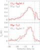 |
Fig. 5 Comparison of HIFI H2O (212 − 101) and (111 − 000) lines (top) at 1669 GHz and 1113 GHz, respectively, and between the H2O (202 − 111) at 988 GHz and the (211 − 202) at 752 GHz lines (bottom). The H2O transitions are labeled in each panel. The vertical dashed line marks the ambient LSR velocity vLSR ~ 2.6 kms-1 (Bachiller & Pérez Gutiérrez 1997). |
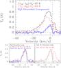 |
Fig. 6 Top: comparison of HIFI spectra for H2O transitions connecting with the ground state: o-H2O (110 − 101) shown by the dashed black line and p-H2O (111 − 000) shown by the thin solid red line. The spectrum shown in blue (solid thick line) is the residual emission after subtracting the emission of p-H2O (111 − 000) line from the o-H2O (110 − 101), referred to as the extended component. Bottom: comparison of the extended component seen in the H2O (110 − 101) line (solid black line) with the o-NH3 (10 − 00) (dashed red line) and the CH3OH (616 − 505) (dotted blue line) spectra obtained from Codella et al. (2010) (left panel). Comparison of the o-H2O (110 − 101) line at 556.9 GHz observed in B1 (extended component; solid black line) and in L1157-B2 (dashed red line) from Vasta et al. (2012). In all panels the vertical dashed line marks the ambient LSR velocity vLSR ~ 2.6 kms-1 (Bachiller & Pérez Gutiérrez 1997). |
3.3. Outflow emission
Figure 6 (top panel) shows that the profile of the o-H2O (110–101) line at 556.9 GHz presents a significant excess of emission at low velocities compared with the two other lines connecting the ground state level (the 212–101 at 1669 GHz and the 111 − 000 at 1113 GHz transitions) that display similar line profiles (see Fig. 5). This is surprising as the lines at 1113 GHz and 1669 GHz are sensitive to somewhat different excitation conditions.
We subtracted the profile of the p-H2O (111 − 000) line from the o-H2O (110 − 101) line and show its residual emission in Fig. 6 (thick spectrum in the top panel). This residual emission has a peak intensity of Tmb ≃ 0.38 K and it peaks at v = 0 kms-1. This component spans a relatively narrow range of velocities, from ~2.6 kms-1 up to −8 kms-1, and its integrated intensity, in Tmb scale, is 2.3 K kms-1.
As can be seen in Fig. 1, the HIFI beam at 1113 GHz and 1669 GHz collects emission from a region at the apex of the bow-shock, with a typical size of ≈10″ (see also Lefloch et al. 2012) whereas the 556.9 GHz also collects emission associated with the B1 cavity walls and the entrained gas, downstream and eastward of the B1 cavity, associated with the B2 ejection. An additional clue on the origin of the extended component is obtained by comparing the 556.9 GHz line profiles of the extended component and the older outflow cavity L1157-B2 (see also Fig. 1) observed by Vasta et al. (2012). As can be seen in Fig. 6 (bottom right panel), both profiles show an excellent match at blueshifted velocities, suggesting a common origin. Interestingly, an excellent match was observed in the CO J = 3–2 profiles of the g3 component and the L1157-B2 shock by Lefloch et al. (2012). Comparison of the line profile of the extended H2O component with the o-NH3 (10 − 00) and CH3OH (616 − 505) lines (Codella et al. 2010), observed at a similar angular resolution with HIFI (~38′′), reveals a very good agreement, supporting the hypothesis that they have a common origin and all trace the same gas. We propose that the broad HIFI beam at 556.9 GHz is actually tracing an extended component, of low excitation, to which the beam of HIFI is less sensitive at the frequency of the H2O lines at 1113 GHz (1669 GHz), as its size decreases from 38′′to  (
( ). This component could represent the counterpart at 556.9 GHz of the plateau observed by PACS, south of B1. Lack of angular resolution prevents us from being more specific about the origin of the extended component, and a comparison with the 556.9 GHz map presented by Bjerkeli et al. (2013) would help to support our interpretation.
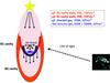 |
Fig. 7 L1157 blue-lobe outflow system. The B1 and B2 outflow cavities are indicated in red and orange, respectively. The two shock components identified through H2O lines are displayed in blue (warm shocked gas) and in light violet for the hot tenuous gas. In the top right corner of the image we show the physical conditions of each component. The observer, represented by the Herschel satellite, is indicated on the right side of the image. |
The H2O emission from the outflow has been recently analyzed by Bjerkeli et al. (2013), who presented a detailed study of the physical properties (molecular mass, dynamical time-scale, momentum, kinetic energy, etc.) in the outflow using CO and H2O lines. In what follows, we will concentrate on the physical conditions in the bow-shock, where the bulk of H2O emission originates.
4. Analysis and discussion
We have determined the physical conditions of the B1 shock region by modeling the water line emission using a radiative transfer code in the large velocity gradient (LVG) approximation. It is worth noting that the B1 shock position is about far away from the protostar L1157-mm; the continuum emission detected in the submm/far-IR range is faint enough that infrared radiative pumping of the H2O lines can be neglected.
We first present our approach to the modeling of the L1157-B1 emission (Sect. 4.1), we then discuss the best-fit solution to the emission from the B1 shock (Sect. 4.2), and we show its consistency with the previous works on CO and H2. We assess the influence of various parameters of the modeling, in particular the actual value of the ortho to para H2 ratio in the shocked gas. Finally, we study the origin of the water absorbing layer in the cloud (Sect. 4.3), and report on the water abundance and far-IR cooling (Sect. 4.4). For the sake of clarity, in Fig. 7 we display the physical structure emerging from our H2O line study that summarizes the main results to be presented in this section. Briefly, we identified five components: the cloud seen in absorption, the outflow material from the B1 (g2) and B2 (g3) cavities, the jet impact shock region (g1), and a compact hot gas component.
Observed and predicted water line fluxes for an OPR H2O = 3.
4.1. Modeling
Previous studies at millimeter and infrared wavelengths (Benedettini et al. 2007; Codella et al. 2009; Takami et al. 2011; and more recently Benedettini et al. 2013) reveal a complex density, temperature, and velocity structure, with several emission knots of shocked gas in various tracers. In such a complex environment, a comprehensive modeling of the water line emission from the bow-shock, notoriously a very difficult task, is just too difficult to handle if one considers the angular resolution of the data (at best comparable to the size of the region), the one-dimensional nature of the source geometrical modeling, and the radiative transfer code used. Our goal here is to identify the main shock components responsible for the H2O emission detected, and, within the uncertainties inherent to the calibration and geometry adopted, the physical conditions of these components.
The PACS maps (Fig. 2) show that the H2O emission does not peak at the nominal position of B1, where the HIFI beam is centered; the larger HIFI beams encompass the emission peak while for the smaller HIFI beams the peak is partially covered (see Fig. 1). It is all the more important to carry out LVG calculations using water fluxes measured over the same source solid angle; we therefore convolved all the PACS maps to a common angular resolution of to measure the flux towards the nominal position of B1. For the HIFI lines, we convolved the o-H2O (212 − 101) PACS map at the resolution of the different HIFI beams. Assuming that all HIFI lines have the same spatial distribution as the o-H2O (212 − 101) line we can then derive the HIFI beam filling factor. As a test, we compared the beam filling factors obtained from PACS maps of the 108, 138, and 125 μm lines. In practice, we obtain very similar correcting factors, which made us feel confident about the robustness of the procedure and the results obtained. The fluxes of all the H2O lines estimated in a beam of are listed in Table 3.
We investigated the excitation conditions of the H2O line emission using a radiative transfer code in the LVG approximation (Ceccarelli et al. 2003) and adopting a plane parallel geometry. The molecular data were taken from the BASECOL4 database (Dubernet et al. 2006, 2013) and we used the new collisional rate coefficients with H2 (Dubernet et al. 2009; Daniel et al. 2010, 2011). The linewidth (FWHM of the line profile) was set to a fixed value of 10 kms-1. The model includes the effects of the beam filling factor, and it computes the reduced chi-square  for each column density minimizing with respect to the source size, kinetic temperature, and density. We adopted an uncertainty in the integrated intensities of 30% for all lines except the HIFI lines with high Eu and the PACS lines lying at the edges of the band, for which the adopted uncertainty is 50%.
4.2. Shock emission: best-fit model
4.2.1. A two-temperature model
The present LVG calculations were carried out for an ortho-to-para ratio (OPR) of 0.5 in the H2 gas, which is close to the value estimated by Nisini et al. (2010b) for gas in the same range of excitation conditions from modeling the H2 emission, and an OPR of the H2O gas equal to 3. We also adopted a size of 10′′, as estimated from the PACS maps, consistent with our previous findings (Benedettini et al. 2012) and with the Spitzer image of L1157-B1 observed in the H2 lines (Nisini et al. 2010b) and in the IRAC bands (Takami et al. 2011).
Physical conditions of the shock components accounting for the water line emission in L1157-B1.
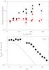 |
Fig. 8 Top: ratio between the measured integrated intensities and the LVG model predictions. Filled circles/triangles depict o-H2O and p-H2O lines, respectively. In black, we display the results assuming one single temperature component (Tkin = 250 K, n(H2) = 106 cm-3, N(o-H2O) = 2 × 1014 cm-2, size = 10′′); in red, the final solution when adding the contribution of the second temperature (Tkin = 1000 K, n(H2) = 2 × 104 cm-3, N(o-H2O) = 7 × 1016 cm-2, size = |
To account for the line fluxes of the three transitions connected to the ground state (ortho and para) and assuming a source size of 10′′, the acceptable range of physical condition is Tkin ~ 200–300 K, n(H2) = (1 − 6) × 106 cm-3, and N(o-H2O) = (0.8 − 2) × 1014. The best-fit model yields a warm gas component at 250 K, n(H2) = 1 × 106 cm-3, N(o-H2O) = 2 × 1014 cm-2. These physical conditions are absolutely unable to account for the flux of lines at higher upper energy levels (see Fig. 8, top panel).
A second gas component, at a much higher temperature and lower density, is needed to reproduce the flux detected in the higher Eu transitions. Solutions with Tkin ≃ 650 K, N(o-H2O) = 1 × 1017 cm-2, n(H2) = 8 × 103 cm-3, and a source size of 4″, are possible, in principle, under the assumption that the OPR-H2 remains unchanged, equal to 0.5. Observational constraints on H2 suggest a higher value of OPR-H2, typically ≃3, at high temperatures (see below). Assuming a typical OPR-H2 of 3 for the second, hot gas component, our modeling favor higher-temperature solutions, with Tkin ≃ 1000 K, N(o-H2O) = 7 × 1016 cm-2, n(H2) = 2 × 104 cm-3, and a size of  as a best-fit model. We found, however, a range of possible solutions, with Tkin ~ 900–1400 K, N(o-H2O) = (3 − 7) × 1016 cm-2, n(H2) = (0.8 − 2) × 104 cm-3, and a size of 2′′–5′′.
Therefore, in addition to the warm dense g1 gas, a small region of hot, low density gas is contributing to the water emission detected by Herschel.
To evaluate the quality of our best-fit model, we have computed the ratio of the measured water line fluxes to those predicted by our model as a function of the upper energy level of the transition. As can be seen in Fig. 8 (top panel), the overall agreement between the measured fluxes and the observations is satisfying; a minimization of our two-temperature model yields  . The water line fluxes resulting from the LVG modeling are reported in Table 3 and the range of physical conditions of the warm (g1) and hot shock gas components are summarized in Table 4. The large number of lines detected at high S/N together with the availability of a wealth of complementary data allow us to constrain the water excitations conditions with unprecedented precision. It is important, however, to note that source sizes have been imposed and this two-component model is a simplification of the complex structure of the bow-shock, in which a wide and continuous range of temperatures and densities are most likely present.
Finally, we evaluated the influence of the OPR-H2O on the results. Only models with an OPR-H2O of 3 (the statistical equilibrium value) can match the observed line fluxes, while a value of 1 always yields solutions with a  >2.
>2.
4.2.2. Influence of the ortho-to-para H2 ratio
In their study of the emission of the pure rotational lines of H2 with Spitzer, Nisini et al. (2010b) found evidence for two gas components at ≈300 K and 1400 K, respectively. They modeled the OPR-H2 as varying continuously from a value of ≈0.6 in gas at 300 K to its value at LTE (=3) in gas at 1400 K. Therefore, we explored the range of acceptable solutions (n,N,T) when considering OPR-H2 as a free parameter. The best-fit solution was obtained for an OPR of 0.5 in the gas at 250 K, hence a value similar to that found by Nisini et al. (2010b) in the gas of moderate excitation. We could not find a reasonable set of physical conditions for values of OPR-H2 higher than 1 for that component.
As noticed by Wilgenbus et al. (2000), such a low value of the OPR-H2 indicates that the gas has been recently heated up by the passage of the shock front, and not affected by an older shock episode since the timescale between shock episodes is much smaller than the timescale needed for the OPR-H2 to return to the equilibrium value. This is consistent with the youth of B1, for which the estimated dynamical age is ~2000 yr (Gueth et al. 1996) and the evolutionary age of the shock model presented by Gusdorf et al. (2008b). Low values of the OPR-H2 have been reported in other outflow shock regions (e.g., Neufeld et al. 1998, 2006; Lefloch et al. 2003; Maret et al. 2009).
As for the second, hot gas component contributing to the water line emission, higher-temperature solutions are favored when adopting an OPR-H2 of 3, and we found satisfying solutions ( = 0.8–1.2) for Tkin ≃ 1000 K, and a gas column density N(H2O) ≃ 9 × 1016 cm-2. The density and the size are less well constrained, with values of the order a few 103 − 4 cm-3 and a few arcsec, respectively.
4.2.3. Modeling consistency
Since our simple model aims at reproducing only the water line fluxes and not the line profiles, one might question its consistency with respect to the spectroscopic information of the line profiles obtained with HIFI. In other words, is there any evidence for specific observational signatures of the two temperature components invoked in our modeling?
From Fig. 8 (top panel), it appears immediately that the bulk of flux of most of the lines in the HIFI and PACS range actually comes from the hot gas component at Tkin ≈ 1000 K. Conversely, the lines at 556.9, 1669, and 1113 GHz (HIFI) are very well accounted for by the warm component at Tkin ≈ 250 K. This is consistent with the two groups of line profiles (1113/1669 GHz and 752/998 GHz) identified (see Fig. 5 in Sect. 3.2). The line profiles are very similar within each group, and differ markedly from one group to the other. Our model provides a simple explanation to this observational fact: we are actually probing two different regions with different excitation conditions.
Second, we have compared our PACS observations with the fluxes predicted by our two-temperature model for all the water lines falling in the range 50–200 μm. As can be seen in Fig. 9, most of the lines remain below the dashed line, which draws the sensitivity limit of the observations. Our model does not predict more lines lying above the sensitivity limit than those actually detected.
The CO line observations with PACS and HIFI revealed a warm, dense gas component, thermalized at 220 K, which Benedettini et al. (2012) and Lefloch et al. (2012) attributed to the jet impact region against the B1 cavity. Both the location and the temperature of this component agree with the properties with the warm gas component identified by Nisini et al. (2010b). However, since the bulk of emission of the CO (16–15) and H2O 1097 GHz lines arises from two components of different excitation inside the B1 cavity, we conclude that the profile of the H2O 1097 GHz line might actually not be specific to g1 and that it indicates a more complex origin of that spectral feature, the opposite of what was claimed in a previous work (Lefloch et al. 2012).
One might wonder why the CO counterpart of the second component is not detected by the sensitive PACS and HIFI instruments. This is illustrated in the bottom panel in Fig. 8, which displays the predicted CO fluxes for the hot component (Tkin ≈ 1000 K, n(H2) = 2 × 104 cm-3, and the assumed size of ), assuming an abundance ratio [CO]/[H2O] = 1. Adopting the standard value of 10-4 for CO would imply a smaller value of the column density, and the flux of the hot component would be even smaller.
We point out that a similar two-component model has recently been presented by Santangelo et al. (2013) to account for the water emission towards the B2 shock position of the L1448 molecular outflow, where the physical conditions are similar to the ones obtained in L1157-B1. Confirming the presence of similar two-component structures in other shock regions would suggest that both components are most likely related to the bow-shock phenomenon itself. The nature of the relation could provide some clues into the origin of the line profiles observed.
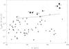 |
Fig. 9 Predicted H2O fluxes in the PACS range of the two-component model, shown in Fig. 8 and Table 3, as a function of wavelength. Black/gray circles and triangles mark the observed/predicted fluxes of o-H2O and p-H2O lines, respectively. Squares represent upper limits of H2O lines listed in Table 2. The line_ID is also shown (see Table 2). The dashed line indicates the sensitivity limit of PACS. |
4.3. Cloud absorption
In Sect. 3.2, we showed that H2O transitions connecting with the ground state level present a narrow self-absorption feature close to the ambient velocity, at vLSR ~ 2.6 kms-1. Since optically thin lines, such as 13CO (Lefloch et al., in prep.) and HDO (Codella et al. 2012), peak close to the ambient velocity, we propose that the absorption feature seen in the low-excited H2O lines most likely arises from an extended layer associated with the cloud envelope, as a result of ice photodesorption. This model was successfully applied by Coutens et al. (2012) to the low-mass Class 0 protostar IRAS 16293–2422, where the authors found a similar self-absorption signature in the fundamental lines of HDO and H O. To account for the observed line profiles, the authors added an absorbing layer in front of the IRAS 16293–2422 envelope that results from the photodesorption of icy mantles at the edge of the cloud by the far-ultraviolet (FUV) photons, as modeled by Hollenbach et al. (2009).
Interpreting the absorption feature in a similar way as due to a water-rich layer caused by ice photodesorption at the cloud surface, we can estimate its water abundance. Caratti o Garatti et al. (2006) evaluate the visual extinction towards the B1 shock through near-IR data and find that AV is, at most, 2 mag. Thus, adopting AV of 1–2 mag, assuming an incident FUV flux of G0 = 1 (i.e., adopting a standard interstellar radiation field), and a typical cloud gas density of 104 cm-3, Hollenbach et al. (2009) predict a water abundance of about ~10-7. At the same depth and for a fixed value of G0, lower densities would result in slightly lower values of the H2O abundance. Instead, if we consider higher values of G0 the water abundance for AV of 1–2 mag will be lower as a higher incident flux modifies the depth of the freeze, moving it towards higher visual extinction, resulting in a peak deeper in the cloud for gas-phase H2O. Therefore, we estimate the water abundance of the cloud absorbing layer to be ≃10-7. Adopting the relation N(H2) = 9.4 × 10²⁰ AV (Frerking et al. 1982) we obtained N(H2) = (0.9–1.9) × 1021 cm-2 for an AV of 1–2 mag, and hence the column density of H2O in this absorbing layer should be about 1 × 1013 cm-2.
4.4. Water abundance and line cooling
The water abundance X(H2O) = [H2O]/[H2] in the shocked gas was derived using the H2 data from Nisini et al. (2010b) obtained with Spitzer and convolved at the PACS resolution (). For the 250 K gas component, the H2 column density was computed from an LTE analysis of the S(0) to S(2) rotational lines. For a source size of 10′′, the column density of H2 is N(H2) ≃ 1.2 × 1020cm-2, which yields a fractional abundance of water ~(0.7–2) × 10-6. This warm gas component is associated with a partly dissociative J-type shock with shock velocities and pre-shock densities, respectively, of either v> 30 kms-1 and 2 × 104 cm-3, or v> 20 kms-1 and 2 × 105 cm-3 (Benedettini et al. 2012; Lefloch et al. 2012), and hence the low water abundance can be explained in terms of FUV photons produced at the shock front; these photons prevent the full conversion of free oxygen into water, and result in a decrease of the water abundance. To obtain the water abundance of the hot gas, we considered the H2 rotational lines S(5) up to S(7) and computed the H2 column density scaled for a source size of . The derived water abundance is (1.2–3.6) × 10-4, in agreement with the predicted values for hot shocked material (Kaufman & Neufeld 1996; Bergin et al. 1998; Flower & Pineau des Forêts 2010). The abundance of H2O in the hot gas is two orders of magnitude higher than that obtained for the warm gas, indicating that all of the available oxygen not locked in CO has been converted to H2O. The derived H2O abundances are reported in Table 4.
The low water abundance associated with the warm gas component confirms previous findings in molecular outflows based on a limited number of lines (e.g., Bjerkeli et al. 2012; Vasta et al. 2012; Tafalla et al. 2013; Santangelo et al. 2013). Moreover, we also confirmed the presence of a hot gas component at higher abundance that so far has been clearly identified only for the B2 shock position of the L1448 outflow (Santangelo et al. 2013). The presence of warm and hot water components have been suggested by Goicoechea et al. (2012) and Dionatos et al. (2013) in shocks close to several Class 0 sources in Serpens. Therefore, our results confirm that in bow-shocks far from the driving source there is a bimodal distribution, which seems to be a common shock characteristic.
Nisini et al. (2010b) obtained the line cooling due to H2 in the B1 shock position, which is on the order5 of 0.03 L⊙. Here, we estimated the total luminosity of water lines, LH2O, from the predicted line fluxes of the best-fit model shown in Fig. 8. We obtained ~0.002 L⊙ and ~0.03 L⊙ for the warm and the hot gas components, respectively. The derived CO luminosity of the warm component is 0.004 L⊙, hence the contribution of water to the line cooling is 50% of the CO luminosity. The luminosity of hot CO gas component, on the other hand, is 0.01 L⊙, and therefore the far-IR cooling of H2O dominates in front of CO, and it contributes equally as the H2 line cooling. The results are summarized in Table 4.
Finally, we calculated the total far-IR cooling in the B1 shock region following the definition of Nisini et al. (2002), where LFIR = LOI + LCO + LH2O + LOH. Using the line fluxes reported by Benedettini et al. (2012), we estimated the total luminosity of [OI] and OH, which are LOI ≃ 2 × 10⁻³L⊙ and LOH ≃ 4 × 10⁻⁴L⊙. For CO and H2O we considered the contribution of the two gas components. One can clearly see that the far-IR cooling is dominated by the contribution of H2O and CO lines, followed by [OI] and OH. The total far-IR cooling estimated in B1 is ~0.05 L⊙. It is worth noticing that the far-IR luminosity has been computed using similar beam sizes for all species, while the H2 luminosity was estimated with a smaller beam.
Shock models produce markedly different predictions on the H2O cooling function, depending on the nature of the shock, either C-type (MHD) or J-type shocks. We make here a simple comparison with the predictions from the steady-state shock models of Flower & Pineau des Forêts (2010), for a shock propagating at v = 20 kms-1 into gas with pre-shock density of 104 cm-3. Our goal is to identify qualitative trends of the properties of the shock responsible for the H2O emission detected. As pointed out by Gueth et al. (1996), the B1 bow-shock propagates into gas previously accelerated by the ejection associated with B2. Maximum velocities of 5–10 kms-1 are reported in the B2 outflow cavity (Vasta et al. 2012). For this reason, we consider that velocities detected in the H2O gas towards B1 (≈30 kms-1; Fig. 4) are not inconsistent with a shock velocity of about 20 kms-1.
For the warm (Tkin ≃ 250 K) gas component, the H2O line cooling is ≈1.5 × 10⁻¹⁹ erg cm-3 s-1, in agreement with the value predicted in the molecular reformation zone of a J-type shock (see Fig. 2 in Flower & Pineau des Forêts 2010; see also Benedettini et al. 2012). For the hot (Tkin ≃ 1000 K) gas component, the H2O line cooling is ≈2 × 10-16 erg cm-3 s-1, a value several orders of magnitude higher than that predicted by the C-shock model, but well in the range of values expected in the J-type shock. Therefore, the simple comparison suggests that the hot gas layer is excited in a non-dissociative J-type shock.
5. Summary and conclusions
As part of the CHESS key program, we have analyzed the H2O emission towards the shock region L1157-B1. A grand total of 13 H2O lines (both ortho and para) have been detected with HIFI and PACS instruments arising from transitions with rather low Eu, from 26.7 K to 319.5 K. The PACS and HIFI observations towards the L1157-B1 bow-shock have revealed the presence of several gas components with different excitation. Our main conclusions can be summarized as follows:
-
1.
The bulk of H2O emission originates in the B1bow-shock.
-
2.
An absorption feature is detected in the line profiles that are connected with the ground state level. It arises from a water-enriched layer (X[H2O] ≃ 10-7) at the surface of the cloud formed as a result of water ice photodesorption from interstellar grain mantles, driven by the external UV photons due to the interstellar radiation field.
-
3.
The LVG analysis of the H2O emission associated with the bright high-excitation region (i.e., the bow-shock) has permitted us to identify two physical components. A warm, dense gas (Tkin ~ 200–300 K, n(H2) ≃ (1–3) × 106 cm-3) component traced mainly by the low-excitation lines of water, with an assumed extent of 10′′. The OPR-H2 in the warm gas is ≃0.5. The hot (Tkin ≃ 1000 K) component is made of tenuous gas at a much lower density (a few 103−4 cm-3) similar to that of the parental cloud. It is much more compact, with a typical size of 2′′ − 5′′. The OPR-H2 in the warm gas is ≃3.0, equal to its value at LTE.
-
4.
These two shock components present marked differences in terms of water enrichment. While the derived abundance in the warm gas is (0.7–2) × 10-6, the water abundance estimated in the hot gas is much higher, around (1.2–3.6) × 10-4, indicating that all available oxygen not locked in CO is driven into H2O. The far-IR cooling of the bow-shock appears to be equally dominated by both H2 and the hot water component.
-
5.
A simple comparison of the water line cooling properties with the steady-state shock models of Flower & Pineau des Forêts (2010) is consistent with a J-type shock origin for both components. The exact nature of the hot water spot and its relation with the jet impact against the cavity remains to be established. The low density of the hot H2O gas suggests that the shock propagates into a region of much lower density, either in the ambient cloud or the outflow cavity gas.
Higher-angular resolution observations are needed to understand the structure of the L1157-B1 bow-shock region. We expect that a detailed, multiline study and comparison of the emission properties of the major cooling agents, CO, H2O and H2 at infrared wavelengths with shock model predictions, will help us to clarify the origin of the different shock components revealed by PACS and HIFI and the relation they hold to each other (Cabrit et al., in prep.).
HIPE is a joint development by the Herschel Science Ground Segment Consortium, consisting of ESA, the NASA Herschel Science Center, and the HIFI, PACS, and SPIRE consortia.
LH2 has been corrected for a distance of 250 pc while in Nisini et al. (2010b) the adopted distance is 440 pc.
Acknowledgments
The authors are grateful to the anonymous referee and the editor, Dr. Malcolm Walmsley, for valuable comments. G.B. is grateful to M. Pereira-Santaella for fruitful discussion. G. Busquet, M. Benedettini, C. Codella, B. Nisini, A. I. Gómez-Ruiz, and A. M. di Giorgio are supported by the Italian Space Agency (ASI) project I/005/11/0. B. Lefloch thanks the Spanish MEC for funding support through grant SAB2009-0011. B. Lefloch, C. Ceccarelli, and L. Wiesenfeld acknowledge funding from the French Space Agency CNES and the National Research Agency funded project FORCOM, ANR-08-BLAN-0225. S. Viti acknowledges support from the [European Community’s] Seventh Framework Programme [FP7/2007-2013] under grant agreement n° 238258. A. Gusdorf acknowledges support by grant ANR-09-BLAN-0231-01 from the French Agence Nationale de la Recherche as part of the SCHISM project. HIFI has been designed and built by a consortium of institutes and university departments from across Europe, Canada and the United States under the leadership of SRON Netherlands Institute for Space Research, Groningen, The Netherlands, and with major contributions from Germany, France and the US. Consortium members are: Canada: CSA, U.Waterloo; France: CESR, LAB, LERMA, IRAM; Germany: KOSMA, MPIfR, MPS; Ireland, NUI Maynooth; Italy: ASI, IFSI-INAF, Osservatorio Astrofisico di Arcetri-INAF; Netherlands: SRON, TUD; Poland: CAMK, CBK; Spain: Observatorio Astronómico Nacional (IGN), Centro de Astrobiología (CSIC-INTA). Sweden: Chalmers University of Technology – MC2, RSS & GARD; Onsala Space Observatory; Swedish National Space Board, Stockholm University – Stockholm Observatory; Switzerland: ETH Zurich, FHNW; USA: Caltech, JPL, NHSC. PACS has been developed by a consortium of institutes led by MPE (Germany) and including UVIE (Austria); KU Leuven, CSL, IMEC (Belgium); CEA, LAM (France); MPIA (Germany); INAF-IFSI/OAA/OAP/OAT, LENS, SISSA (Italy); IAC (Spain). This development has been supported by the funding agencies BMVIT (Austria), ESA-PRODEX (Belgium), CEA/CNES (France), DLR (Germany), ASI/INAF (Italy), and CICYT/MCYT (Spain).
References
- Arce, H. G., Santiago-García, J., Jørgensen, J. K., Tafalla, M., & Bachiller, R. 2008, ApJ, 681, L21 [NASA ADS] [CrossRef] [Google Scholar]
- Bachiller, R. 1996, ARA&A, 34, 111 [NASA ADS] [CrossRef] [Google Scholar]
- Bachiller, R., & Pérez Gutiérrez, M. 1997, ApJ, 487, L93 [NASA ADS] [CrossRef] [Google Scholar]
- Bachiller, R., Pérez Gutiérrez, M., Kumar, M. S. N., & Tafalla, M. 2001, A&A, 372, 899 [NASA ADS] [CrossRef] [EDP Sciences] [Google Scholar]
- Benedettini, M., Viti, S., Codella, C., et al. 2007, MNRAS, 381, 1127 [NASA ADS] [CrossRef] [Google Scholar]
- Benedettini, M., Busquet, G., Lefloch, B., et al. 2012, A&A, 539, L3 [NASA ADS] [CrossRef] [EDP Sciences] [Google Scholar]
- Benedettini, M., Viti, S., Codella, C., et al. 2013, MNRAS, 436, 179 [NASA ADS] [CrossRef] [Google Scholar]
- Bergin, E. A., Neufeld, D. A., & Melnick, G. J. 1998, ApJ, 499, 777 [NASA ADS] [CrossRef] [MathSciNet] [Google Scholar]
- Bjerkeli, P., Liseau, R., Olberg, M., et al. 2009, A&A, 507, 1455 [NASA ADS] [CrossRef] [EDP Sciences] [Google Scholar]
- Bjerkeli, P., Liseau, R., Larsson, B., et al. 2012, A&A, 546, A29 [NASA ADS] [CrossRef] [EDP Sciences] [Google Scholar]
- Bjerkeli, P., Liseau, R., Nisini, B., et al. 2013, A&A, 552, L8 [NASA ADS] [CrossRef] [EDP Sciences] [Google Scholar]
- Caratti o Garatti, A., Giannini, T., Nisini, B., & Lorenzetti, D. 2006, A&A, 449, 1077 [NASA ADS] [CrossRef] [EDP Sciences] [Google Scholar]
- Ceccarelli, C., Maret, S., Tielens, A. G. G. M., Castets, A., & Caux, E. 2003, A&A, 410, 587 [NASA ADS] [CrossRef] [EDP Sciences] [Google Scholar]
- Ceccarelli, C., Bacmann, A., Boogert, A., et al. 2010, A&A, 521, L22 [NASA ADS] [CrossRef] [EDP Sciences] [Google Scholar]
- Codella, C., Benedettini, M., Beltrán, M. T., et al. 2009, A&A, 507, L25 [NASA ADS] [CrossRef] [EDP Sciences] [Google Scholar]
- Codella, C., Lefloch, B., Ceccarelli, C., et al. 2010, A&A, 518, L112 [NASA ADS] [CrossRef] [EDP Sciences] [Google Scholar]
- Codella, C., Ceccarelli, C., Lefloch, B., et al. 2012, ApJ, 757, L9 [NASA ADS] [CrossRef] [Google Scholar]
- Coutens, A., Vastel, C., Caux, E., et al. 2012, A&A, 539, A132 [NASA ADS] [CrossRef] [EDP Sciences] [Google Scholar]
- Daniel, F., Dubernet, M.-L., Pacaud, F., & Grosjean, A. 2010, A&A, 517, A13 [NASA ADS] [CrossRef] [EDP Sciences] [Google Scholar]
- Daniel, F., Dubernet, M.-L., & Grosjean, A. 2011, A&A, 536, A76 [NASA ADS] [CrossRef] [EDP Sciences] [Google Scholar]
- Davis, C. J., & Eisloeffel, J. 1995, A&A, 300, 851 [NASA ADS] [Google Scholar]
- de Graauw, T., Helmich, F. P., Phillips, T. G., et al. 2010, A&A, 518, L6 [NASA ADS] [CrossRef] [EDP Sciences] [Google Scholar]
- Dionatos, O., Jørgensen, J. K., Green, J. D., et al. 2013, A&A, 558, A88 [NASA ADS] [CrossRef] [EDP Sciences] [Google Scholar]
- Draine, B. T., Roberge, W. G., & Dalgarno, A. 1983, ApJ, 264, 485 [NASA ADS] [CrossRef] [Google Scholar]
- Dubernet, M.-L., Grosjean, A., Flower, D., et al. 2006, Journal of Plasma Research SERIES, 7, 356 [Google Scholar]
- Dubernet, M.-L., Daniel, F., Grosjean, A., & Lin, C. Y. 2009, A&A, 497, 911 [NASA ADS] [CrossRef] [EDP Sciences] [Google Scholar]
- Dubernet, M.-L., Alexander, M. H., Ba, Y. A., et al. 2013, A&A, 553, A50 [NASA ADS] [CrossRef] [EDP Sciences] [Google Scholar]
- Flower, D. R., & Pineau des Forêts, G. 2010, MNRAS, 406, 1745 [NASA ADS] [Google Scholar]
- Flower, D. R., & Pineau des Forêts, G. 2012, MNRAS, 421, 2786 [NASA ADS] [CrossRef] [Google Scholar]
- Franklin, J., Snell, R. L., Kaufman, M. J., et al. 2008, ApJ, 674, 1015 [NASA ADS] [CrossRef] [Google Scholar]
- Frerking, M. A., Langer, W. D., & Wilson, R. W. 1982, ApJ, 262, 590 [NASA ADS] [CrossRef] [Google Scholar]
- Giannini, T., Nisini, B., & Lorenzetti, D. 2001, ApJ, 555, 40 [NASA ADS] [CrossRef] [Google Scholar]
- Goicoechea, J. R., Cernicharo, J., Karska, A., et al. 2012, A&A, 548, A77 [NASA ADS] [CrossRef] [EDP Sciences] [Google Scholar]
- Gueth, F., Guilloteau, S., & Bachiller, R. 1996, A&A, 307, 891 [NASA ADS] [Google Scholar]
- Gueth, F., Guilloteau, S., & Bachiller, R. 1998, A&A, 333, 287 [NASA ADS] [Google Scholar]
- Gusdorf, A., Cabrit, S., Flower, D. R., & Pineau des Forêts, G. 2008a, A&A, 482, 809 [Google Scholar]
- Gusdorf, A., Pineau des Forêts, G., Cabrit, S., & Flower, D. R. 2008b, A&A, 490, 695 [NASA ADS] [CrossRef] [EDP Sciences] [Google Scholar]
- Hollenbach, D., & McKee, C. F. 1989, ApJ, 342, 306 [NASA ADS] [CrossRef] [Google Scholar]
- Hollenbach, D., Kaufman, M. J., Bergin, E. A., & Melnick, G. J. 2009, ApJ, 690, 1497 [CrossRef] [Google Scholar]
- Kaufman, M. J., & Neufeld, D. A. 1996, ApJ, 456, 611 [NASA ADS] [CrossRef] [Google Scholar]
- Lefloch, B., Cernicharo, J., Cabrit, S., et al. 2003, ApJ, 590, L41 [NASA ADS] [CrossRef] [Google Scholar]
- Lefloch, B., Cabrit, S., Busquet, G., et al. 2012, ApJ, 757, L25 [NASA ADS] [CrossRef] [Google Scholar]
- Looney, L. W., Tobin, J. J., & Kwon, W. 2007, ApJ, 670, L131 [NASA ADS] [CrossRef] [Google Scholar]
- Maret, S., Bergin, E. A., Neufeld, D. A., et al. 2009, ApJ, 698, 1244 [NASA ADS] [CrossRef] [Google Scholar]
- Neufeld, D. A., Melnick, G. J., & Harwit, M. 1998, ApJ, 506, L75 [NASA ADS] [CrossRef] [Google Scholar]
- Neufeld, D. A., Melnick, G. J., Sonnentrucker, P., et al. 2006, ApJ, 649, 816 [NASA ADS] [CrossRef] [Google Scholar]
- Neufeld, D. A., Nisini, B., Giannini, T., et al. 2009, ApJ, 706, 170 [NASA ADS] [CrossRef] [Google Scholar]
- Nisini, B., Giannini, T., & Lorenzetti, D. 2002, ApJ, 574, 246 [NASA ADS] [CrossRef] [Google Scholar]
- Nisini, B., Codella, C., Giannini, T., et al. 2007, A&A, 462, 163 [NASA ADS] [CrossRef] [EDP Sciences] [Google Scholar]
- Nisini, B., Benedettini, M., Codella, C., et al. 2010a, A&A, 518, L120 [NASA ADS] [CrossRef] [EDP Sciences] [Google Scholar]
- Nisini, B., Giannini, T., Neufeld, D. A., et al. 2010b, ApJ, 724, 69 [NASA ADS] [CrossRef] [Google Scholar]
- Ott, S. 2010, in Astronomical Data Analysis Software and Systems XIX, eds. Y. Mizumoto, K.-I. Morita, & M. Ohishi, ASP Conf. Ser., 434, 139 [Google Scholar]
- Pickett, H. M., Poynter, R. L., Cohen, E. A., et al. 1998, J. Quant. Spectr. Rad. Transf., 60, 883 [NASA ADS] [CrossRef] [Google Scholar]
- Pilbratt, G. L., Riedinger, J. R., Passvogel, T., et al. 2010, A&A, 518, L1 [CrossRef] [EDP Sciences] [Google Scholar]
- Poglitsch, A., Waelkens, C., Geis, N., et al. 2010, A&A, 518, L2 [NASA ADS] [CrossRef] [EDP Sciences] [Google Scholar]
- Roelfsema, P. R., Helmich, F. P., Teyssier, D., et al. 2012, A&A, 537, A17 [NASA ADS] [CrossRef] [EDP Sciences] [Google Scholar]
- Santangelo, G., Nisini, B., Antoniucci, S., et al. 2013, A&A, 557, A22 [NASA ADS] [CrossRef] [EDP Sciences] [Google Scholar]
- Tafalla, M., & Bachiller, R. 1995, ApJ, 443, L37 [Google Scholar]
- Tafalla, M., Liseau, R., Nisini, B., et al. 2013, A&A, 551, A116 [NASA ADS] [CrossRef] [EDP Sciences] [Google Scholar]
- Takami, M., Karr, J. L., Nisini, B., & Ray, T. P. 2011, ApJ, 743, 193 [NASA ADS] [CrossRef] [Google Scholar]
- van Dishoeck, E. F., Kristensen, L. E., Benz, A. O., et al. 2011, PASP, 123, 138 [NASA ADS] [CrossRef] [Google Scholar]
- Vasta, M., Codella, C., Lorenzani, A., et al. 2012, A&A, 537, A98 [NASA ADS] [CrossRef] [EDP Sciences] [Google Scholar]
- Wilgenbus, D., Cabrit, S., Pineau des Forêts, G., & Flower, D. R. 2000, A&A, 356, 1010 [NASA ADS] [Google Scholar]
- Zhang, Q., Ho, P. T. P., & Wright, M. C. H. 2000, AJ, 119, 1345 [NASA ADS] [CrossRef] [Google Scholar]
All Tables
Physical conditions of the shock components accounting for the water line emission in L1157-B1.
All Figures
|
Fig. 1 Southern blueshifted outflow lobe observed in CO (1–0) with the Plateau de Bure Interferometer (PdBI) by Gueth et al. (1996). The black cross marks the nominal position of the bow-shock L1157-B1 while the white × symbol indicates the nominal position of the B2 shock (Bachiller & Pérez Gutiérrez 1997). The largest (~38′′) and smallest (~12 |
| In the text | |
|
Fig. 2 PACS maps of H2O line fluxes (increasing upper-level energy from top left to bottom right). First contour corresponds to the 1σ flux level of each transition. The contour step is 2σ in all lines except for the o-H2O (212 − 101) and o-H2O (303 − 212), for which the contour step is 6σ and 3σ, respectively, where σ is listed in Table 2. The top right panel shows an overlay of the o-H2O (212 − 101) map (gray scale) with the PdBI CH3CN (8–7) K = 0–2 image (red contours) from Codella et al. (2009) tracing the bow-shock. The synthesized beam of PdBI, |
| In the text | |
|
Fig. 3 Contour maps of the SiO (2–1) high-velocity (v< − 8 kms-1) emission from Gueth et al. (1998) convolved to the |
| In the text | |
|
Fig. 4 HIFI H2O spectra of L1157-B1 smoothed to a velocity resolution of 1 kms-1. The H2O transition is indicated in each panel. The vertical dashed line marks the ambient LSR velocity vLSR ~ 2.6 kms-1 from C18O emission (Bachiller & Pérez Gutiérrez 1997). |
| In the text | |
|
Fig. 5 Comparison of HIFI H2O (212 − 101) and (111 − 000) lines (top) at 1669 GHz and 1113 GHz, respectively, and between the H2O (202 − 111) at 988 GHz and the (211 − 202) at 752 GHz lines (bottom). The H2O transitions are labeled in each panel. The vertical dashed line marks the ambient LSR velocity vLSR ~ 2.6 kms-1 (Bachiller & Pérez Gutiérrez 1997). |
| In the text | |
|
Fig. 6 Top: comparison of HIFI spectra for H2O transitions connecting with the ground state: o-H2O (110 − 101) shown by the dashed black line and p-H2O (111 − 000) shown by the thin solid red line. The spectrum shown in blue (solid thick line) is the residual emission after subtracting the emission of p-H2O (111 − 000) line from the o-H2O (110 − 101), referred to as the extended component. Bottom: comparison of the extended component seen in the H2O (110 − 101) line (solid black line) with the o-NH3 (10 − 00) (dashed red line) and the CH3OH (616 − 505) (dotted blue line) spectra obtained from Codella et al. (2010) (left panel). Comparison of the o-H2O (110 − 101) line at 556.9 GHz observed in B1 (extended component; solid black line) and in L1157-B2 (dashed red line) from Vasta et al. (2012). In all panels the vertical dashed line marks the ambient LSR velocity vLSR ~ 2.6 kms-1 (Bachiller & Pérez Gutiérrez 1997). |
| In the text | |
|
Fig. 7 L1157 blue-lobe outflow system. The B1 and B2 outflow cavities are indicated in red and orange, respectively. The two shock components identified through H2O lines are displayed in blue (warm shocked gas) and in light violet for the hot tenuous gas. In the top right corner of the image we show the physical conditions of each component. The observer, represented by the Herschel satellite, is indicated on the right side of the image. |
| In the text | |
|
Fig. 8 Top: ratio between the measured integrated intensities and the LVG model predictions. Filled circles/triangles depict o-H2O and p-H2O lines, respectively. In black, we display the results assuming one single temperature component (Tkin = 250 K, n(H2) = 106 cm-3, N(o-H2O) = 2 × 1014 cm-2, size = 10′′); in red, the final solution when adding the contribution of the second temperature (Tkin = 1000 K, n(H2) = 2 × 104 cm-3, N(o-H2O) = 7 × 1016 cm-2, size = |
| In the text | |
|
Fig. 9 Predicted H2O fluxes in the PACS range of the two-component model, shown in Fig. 8 and Table 3, as a function of wavelength. Black/gray circles and triangles mark the observed/predicted fluxes of o-H2O and p-H2O lines, respectively. Squares represent upper limits of H2O lines listed in Table 2. The line_ID is also shown (see Table 2). The dashed line indicates the sensitivity limit of PACS. |
| In the text | |
Current usage metrics show cumulative count of Article Views (full-text article views including HTML views, PDF and ePub downloads, according to the available data) and Abstracts Views on Vision4Press platform.
Data correspond to usage on the plateform after 2015. The current usage metrics is available 48-96 hours after online publication and is updated daily on week days.
Initial download of the metrics may take a while.