| Issue |
A&A
Volume 561, January 2014
|
|
|---|---|---|
| Article Number | A83 | |
| Number of page(s) | 10 | |
| Section | Interstellar and circumstellar matter | |
| DOI | https://doi.org/10.1051/0004-6361/201322172 | |
| Published online | 06 January 2014 | |
SDC13 infrared dark clouds: Longitudinally collapsing filaments?⋆,⋆⋆,⋆⋆⋆
1
School of Physics & Astronomy, Cardiff University,
Queens Buildings, The parade,
Cardiff
CF24 3AA,
UK
e-mail:
This email address is being protected from spambots. You need JavaScript enabled to view it.
2
Laboratoire AIM, CEA/DSM-CNRS-Universté Paris Diderot, IRFU/Service d’Astrophysique,
C. E.
Saclay, 91191
Gif-sur-Yvette Cedex,
France
3
Jodrell Bank Centre for Astrophysics, School of Physics and
Astronomy, University of Manchester, Manchester, M13
9PL, UK
4
IAS, CNRS (UMR 8617), Université Paris-Sud,
Bâtiment 121,
91400
Orsay,
France
5
Centro de Astrobiología (CSIC-INTA), Ctra. de Torrejón-Ajalvir,
km. 4, 28850 Torrejón de Ardoz, Madrid, Spain
6
Institut de Radioastronomie Millimétrique,
300 Rue de la piscine, 38406
Saint-Martin-d’Hères, France
7
Universidad de Granada, 18071
Granada,
Spain
8
Max-Planck Institut für Radioastronomie,
Auf dem Hügel, 69,
53121
Bonn,
Germany
9
School of Physics and Astronomy, University of Leeds,
Leeds
LS2 9JT,
UK
10
Departamento de Astronomía, Universidad de Chile,
36-D Casilla, Santiago, Chile
11
Instituto de Astrofísica de Canarias, 38200, La Laguna, Tenerife, Spain
12
Universidad de la Laguna, Dept. Astrofisica, 38206 La Laguna,
Tenerife,
Spain
13
Centre for Astrophysics Research, University of Hertfordshire,
College Lane,
Hatfield, Herts,
AL10 9AB,
UK
Received:
28
June
2013
Accepted:
31
October
2013
Abstract
Formation of stars is now believed to be tightly linked to the dynamical evolution of interstellar filaments in which they form. In this paper we analyze the density structure and kinematics of a small network of infrared dark filaments, SDC13, observed in both dust continuum and molecular line emission with the IRAM 30 m telescope. These observations reveal the presence of 18 compact sources amongst which the two most massive, MM1 and MM2, are located at the intersection point of the parsec-long filaments. The dense gas velocity and velocity dispersion observed along these filaments show smooth, strongly correlated, gradients. We discuss the origin of the SDC13 velocity field in the context of filament longitudinal collapse. We show that the collapse timescale of the SDC13 filaments (from 1 Myr to 4 Myr depending on the model parameters) is consistent with the presence of Class I sources in them, and argue that, on top of bringing more material to the centre of the system, collapse could generate additional kinematic support against local fragmentation, helping the formation of starless super-Jeans cores.
Key words: stars: formation / ISM: clouds / ISM: kinematics and dynamics / ISM: structure
Based on observations carried out with the IRAM 30 m Telescope. IRAM is supported by INSU/CNRS (France), MPG (Germany), and IGN (Spain).
Figure 3 and Appendices are available in electronic form at http://www.aanda.org
The FITS files for the N2H+(1–0) Spectra of Fig. 3 are only available at the CDS via anonymous ftp to cdsarc.u-strasbg.fr (130.79.128.5) or via http://cdsarc.u-strasbg.fr/viz-bin/qcat?J/A+A/561/A83
© ESO, 2014
1. Introduction
In recent years, interstellar filaments have received special attention. The far-infrared
Herschel space observatory revealed the ubiquity of filaments in both
quiescent and active star-forming clouds. The detailed analysis of large samples of
filaments identified with Herschel suggest that they represent a key stage
in the formation of low-mass prestellar cores (Arzoumanian et
al. 2011). In the picture proposed by André et al.
(2010), these cores form out of filaments that have reached the thermal critical
mass-per-unit-length,  (Ostriker 1964), above which filaments become
gravitationally unstable. Filaments with
(Ostriker 1964), above which filaments become
gravitationally unstable. Filaments with  are called
supercritical filaments. While this scenario might apply to the bulk of the low-mass
prestellar cores, it can hardly account for the formation of super-Jeans cores (e.g. Sadavoy et al. 2010) whose mass is several times higher
than the local thermal Jeans mass
are called
supercritical filaments. While this scenario might apply to the bulk of the low-mass
prestellar cores, it can hardly account for the formation of super-Jeans cores (e.g. Sadavoy et al. 2010) whose mass is several times higher
than the local thermal Jeans mass  (~1
M⊙ for critical 10 K filaments). Additional support (magnetic,
kinematic) and/or significant subsequent core accretion are needed to explain the formation
of cores with masses
(~1
M⊙ for critical 10 K filaments). Additional support (magnetic,
kinematic) and/or significant subsequent core accretion are needed to explain the formation
of cores with masses  .
.
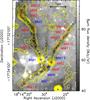 |
Fig. 1 Spitzer 8 μm image of SDC13 in grey scale on top of which we overlaid the IRAM 30 m MAMBO 1.2 mm dust continuum contours (from 3 mJy/beam to 88 mJy/beam in step of 5 mJy/beam). The positions of the identified 1.2 mm compact sources within the SDC13 filaments are marked as crosses, red for starless sources and blue for protostellar sources. |
Several high-resolution studies of filamentary cloud kinematics have been performed in the past three years towards low-mass, nearby, star-forming regions (e.g. Duarte-Cabral et al. 2010; Hacar & Tafalla 2011; Kirk et al. 2013; Arzoumanian et al. 2013). These studies demonstrate the importance of cloud kinematics in the context of filament evolution and core formation. For instance, Kirk et al. (2013) showed that gas filamentary accretion towards the central cluster of young stellar objects (YSOs) in Serpens South could sustain the star formation rate observed in this cloud, providing enough material to constantly form new generations of YSOs. But, it is not clear that these inflows have any impact at all in determining the mass of individual low-mass cores. On the high-mass side, infrared dark clouds (IRDCs) have been privileged targets (e.g. Miettinen 2012; Ragan et al. 2012; Henshaw et al. 2013; Busquet et al. 2013; Peretto et al. 2013). These sources are typically located at a distance of ~4 kpc from the Sun (Peretto & Fuller 2010), making the analysis of filament kinematics more difficult. Thanks to the high sensitivity and resolution of ALMA, Peretto et al. (2013) showed that the global collapse of the SDC335.579-0.292 IRDC is responsible for the formation of an early O-type star progenitor (M ≃ 545 M⊙ in 0.05 pc) sitting at the cloud centre.
In this paper, we present results of an IRDC (hereafter called SDC13), composed of three Spitzer dark clouds from the Peretto & Fuller (2009) catalogue (SDC13.174-0.07, SDC13.158-0.073, SDC13.194-0.073). The near kinematical distance of SDC13 is d = 3.6(±0.4) kpc using the Reid et al. (2009) model. From 8 μm extinction we estimate a total gas mass of ~600 M⊙ above NH2 > 1022 cm-2. As for any IRDC, SDC13 shows little star formation activity, except in the central region where extended infrared emission is observed (see Fig. 1 from Peretto & Fuller 2010). The high extinction contrast, the rather simple geometry, and the high aspect ratios of the SDC13 filaments are remarkable and provide a great opportunity to better understand the impact of filament kinematics on the formation of cores in an intermediate mass regime.
2. Millimetre observations
2.1. Dust continuum data
In December 2009 we observed SDC13 at the IRAM 30 m telescope using the MAMBO bolometer array at 1.2 mm. We performed on-the-fly mapping of a 5′ × 5′ region. The sky opacity at 225 GHz was measured to be between 0.08 and 0.26 depending on the scan. Pointing accuracy was better than 2′′ and calibration on Uranus was better than 10%. We used MOPSIC to reduce these MAMBO data, obtaining a final rms noise level on the reduced image of ~1 mJy/11′′-beam.
We also make use of publicly available Spitzer GLIMPSE (Churchwell et al. 2009) and 24 μm MIPSGAL (Carey et al. 2009) data.
2.2. Molecular line data
In September 2011, during the IRAM 30 m summer school, we observed SDC13 with the IRAM 30 m telescope using the EMIR heterodyne receiver. We performed 31 single-pointing observations along the SDC13 filaments in N2H+(1–0), at 93.2 GHz (i.e. 27′′ beam). The off positions, taken 5′ away from SDC13, were checked to ensure no emission was present there. The pointing was better than 5′′ and the sky opacity was varying between 0.3 to 2 at 225 GHz. We used the FTS spectrometer with a 50 KHz spectral resolution. The data were reduced in CLASS1. The resulting spectra have an rms noise varying from 0.05 to 0.1 K in a 0.16 km s-1 channel width.
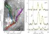 |
Fig. 2 Left: Spitzer 8 μm image of
SDC13 in grey scale on top of which we marked the 31 single-pointing positions we
observed in N2H+(1–0), and the skeletons of each filament
(thick solid lines). The size of the black circles represents the 30 m beam size at
3.2 mm. Right: examples of three N2H+(1–0)
spectra (displayed on |

3. Analysis
3.1. Mass partition in SDC13
The MAMBO observations of SDC13 are presented in Fig. 1. We can see that the 1.2 mm dust continuum emission towards SDC13 matches the mid-infrared extinction very well. In the remainder of this paper we focus only on the emission towards these dark filaments and ignore any other significant emission peaks since we do not have kinematical information for those.
We segmented the emission on this dust continuum map into four filaments: Fi-SE, Fi-NW, Fi-NEs, Fi-NEn. The skeletons of these filaments (Fig. 2-left) were obtained by fitting polynomial functions to the MAMBO emission peaks along them. The splitting of Fi-NE into two parts is due to its dynamical structure (cf. Sect. 3.2). These filaments are barely resolved in our MAMBO map and are responsible for most of the 1.2 mm flux in the region. Although ground-based dust continuum observations filter out all emission whose spatial scale is larger than the size of the bolometer array (~2′ for MAMBO), inspection of Herschel Hi-GAL observations (Molinari et al. 2010) shows that the SDC13 mass is indeed mostly concentrated within the filaments. The observed properties of the filaments (as measured within the 3 mJy/beam contour) are presented in Table 12.
Observed properties of SDC13 filaments.
Using the source identification scheme presented in Appendix A of Peretto & Fuller (2009) we further identified 18 compact sources sitting within the filaments. The observed properties of these sources are given in Table 2. A number of sources have sizes that are close to, or even smaller than, the beam size (all sources with dashes in Table 2 are in this situation). These sources have significant emission peaks (>3σ), but because they are blended with nearby sources, their measured sizes appear smaller than the beam, and their properties are very uncertain. All these sources are confirmed with a higher resolution extinction map and SABOCA data (not shown here). The flux uncertainties in Table 1 reflect the difficulty of estimating the separation between the sources and the underlying filament. It is calculated by taking the average of the clipping and the bijection schemes of the flux estimates (Rosolowsky et al. 2008). We characterised the compact sources further by checking their association with Spitzer 24 μm point-like sources, and their fragmentation as seen in the 8 μm extinction map (see Fig. 1 from Peretto & Fuller 2010). We find that most of the sources are starless (13 out of 18) and that only MM10 appears to be sub-fragmented in extinction. The results of this analysis are also quoted in Table 2.
Observed properties of SDC13 cores.
Physical properties of SDC13 filaments.
Assuming that the dust emission is optically thin at 1.2 mm, the measured fluxes provide a direct measurement of the source mass. In Tables 3 and 4 we give the masses of all structures estimated using a specific dust opacity at 1.2 mm κ1.2 mm = 0.005 cm2 g-1, and dust temperatures of 12 K for filaments and starless sources, and 15 K for protostellar ones (Peretto et al. 2010). We also provide their volume densities, and the mass per unit length of filaments. All uncertainties result from propagation of the flux uncertainties. They do not take systematic uncertainties on the dust temperature/opacity into account, increasing the uncertainty on all calculated properties by an extra factor of ≤2.
3.2. Dense gas projected velocity field
The N2H+(1–0) spectra observed along the SDC13 filaments are displayed in Figs. 2 and 3. All spectra show strong detections (S/N ≥ 4) for all hyperfine line components and symmetric line profiles. Based on these observations, we estimated the systemic velocity of SDC13 at +37 km s-1 (near position 8 in Fig. 2). From position 18 to 24 and 28 to 31, we observe a secondary velocity component separated by +17 km s-1. In Fig. 2 it can be identified as a small bump at V ≃ +54 km s-1 on spectrum #24. This higher velocity component most likely belongs to another cloud on the eastern side of SDC13 that overlaps, in projection, with the Fi-NE filament. For the remainder of the paper have we decided to ignore this higher velocity component.
We used the hyperfine structure line fitting routine of the CLASS software to derive line parameters, such as the centroid gas velocity and gas velocity dispersion (see Fig. 2). We represent the results from this fitting procedure in Fig. 4. The colour and size of the circular symbols code the line-of-sight velocity and linewidth, respectively, of the gas as measured in N2H+(1–0). The exact values are given in Table 5 for each position. Figure 4 shows that both the dense gas velocity and velocity dispersion vary smoothly along each filament, from one end to the other. The two quantities are strongly correlated. Along Fi-NE, we can actually see that the smooth variation in the velocity reaches a minimum (around position 25) to start increasing again towards position 31. We believe that this shows that the northern and southern parts of Fi-NE are dynamically distinct. This is why we decided to subdivide this filament in two, Fi-NEn and Fi-NEs. The Fi-NE filaments are blue-shifted with respect to the systemic velocity of SDC13 while the Fi-NW and Fi-SE filaments are red-shifted. The filaments spatially and dynamically converge near position 8 at the systemic velocity of the system, i.e. +37 km s-1. At this same position, the linewidth reaches a maximum of ~2 km s-1, while at the filament ends the linewidth is the narrowest, i.e. ~0.7 km s-1.
Physical properties of SDC13 cores.
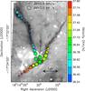 |
Fig. 4 Spitzer 8 μm image of SDC13 in grey scale on top of which we symbolised the results of the N2H+(1–0) HFS fitting as circles. The colour of the symbols indicate the gas velocity while their sizes indicate the gas velocity dispersion (FWHM). |
4. Discussion
4.1. Timescales and filament stability
The Spitzer protostellar objects that we identify in SDC13 filaments are
typically embedded Class I (or young Class II) objects (see Appendix B). The age
τCI of such objects from prestellar core stage to Class I
protostellar stage is 1 Myr ≤ τCI ≤ 2 Myr (e.g. Kirk et al. 2005; Evans
et al. 2009), consequently setting a lower limit of 1 Myr for the age of the
filaments themselves. Their widths3 as measured on
the MAMBO map are ~0.3 pc. Taking a 3D velocity dispersion
 km s-1, we obtain a crossing time
tcross = 0.3(±0.1) Myr. Given their lower age limit of 1
Myr, the SDC13 filaments must therefore either be gravitationally bound or confined by
ram/magnetic pressure. The thermal critical mass-per-unit-length for a 12 K isothermal
filament is
km s-1, we obtain a crossing time
tcross = 0.3(±0.1) Myr. Given their lower age limit of 1
Myr, the SDC13 filaments must therefore either be gravitationally bound or confined by
ram/magnetic pressure. The thermal critical mass-per-unit-length for a 12 K isothermal
filament is  M⊙/pc,
and the observed values for the SDC13 filaments are higher by a factor of 4 to 8 (cf.
Table 3), meaning that they are thermally
supercritical. However, if we consider non-thermal motions as an extra support against
gravity, the picture slightly changes. We define the effective critical
mass-per-unit-length as
M⊙/pc,
and the observed values for the SDC13 filaments are higher by a factor of 4 to 8 (cf.
Table 3), meaning that they are thermally
supercritical. However, if we consider non-thermal motions as an extra support against
gravity, the picture slightly changes. We define the effective critical
mass-per-unit-length as  /G,
where
/G,
where  corresponds to the average total velocity dispersion along the filaments. Taking
 km s-1 (cf. Table
5), we obtain
km s-1 (cf. Table
5), we obtain
 for all filaments, suggesting
that they are critical. This ratio is probably slightly overestimated since the
contribution from the longitudinal collapse of filaments (see following sections) probably
contributes to the observed line widths in the form of non-supportive bulk motions. The
SDC13 filaments match the relationship between Mline and
for all filaments, suggesting
that they are critical. This ratio is probably slightly overestimated since the
contribution from the longitudinal collapse of filaments (see following sections) probably
contributes to the observed line widths in the form of non-supportive bulk motions. The
SDC13 filaments match the relationship between Mline and
 found by
Arzoumanian et al. (2013) for thermally
supercritical filaments.
found by
Arzoumanian et al. (2013) for thermally
supercritical filaments.
N2H+(1–0) spectra properties.
4.2. Dynamical evolution scenarios
The smooth velocity structure observed along the SDC13 filaments shows that these filaments are dynamically coherent. The number of physical processes leading to a well organised parsec-scale velocity pattern, as observed in SDC13, is rather limited. Collapse, expansion, rotation, soft filament collision, and wind-driven acceleration are the five main possibilities. Rotation would imply that the SDC13 filaments rotate about an axis going through the filament junction. The resulting geometry is unrealistic in the context of interstellar cloud dynamics, because differential rotation would tear apart each filament in a crossing time tcross ≃ 0.3 Myr (cf. Sect. 4.1). No expanding source of energy (such as HII region or cluster of outflows4) is located at the centre of SDC13, rendering the expansion scenario unlikely, while colliding filaments cannot account for the velocity pattern observed along Fi-NEn. Finally, wind-driven acceleration powered by a nearby stellar cluster is a credible scenario. In particular, as we can see in Fig. 1 a mid-infrared nebulosity, along with a number of infrared compact sources, are observed east of MM1, probably interacting with it and affecting its velocity through expanding winds. However, it probably does not affect the dynamics of the entire network of filaments. Similar to the colliding flow scenario, the wind-driven scenario can hardly explain the smooth velocity field observed in these filaments and, in particular, the one along Fi-NEn.
We therefore consider that longitudinal collapse is the best option to explain the velocity structure observed in SDC13. Gravity can naturally account for a velocity gradient along the filaments as the gas collapses towards the centre of the system. In this context, one can argue that there is a primary gravitational potential well centre near position 8, towards which all the gas is collapsing, and a secondary one near position 31 towards which only Fi-NEn is infalling. In this collapse scenario, the red-shifted filaments, i.e. Fi-NW and Fi-SE, are in the foreground with respect to the primary centre of the system, while the blue-shifted ones, Fi-NEs and Fi-NEn, are in the background. The dense gas velocity observed along the filaments is therefore interpreted as a projected infall velocity profile. Figure 5 displays these profiles for all four filaments. We can see that for each filament the velocity is a linear function of the distance to the centre (gradients are given in Table 3) up to ~1.5 pc and then flattens out. This is expected when homologous free-fall collapse of filament have centrally concentrated density profiles along their crest (see Fig. 6 from Pon et al. 2011; Fig. 5 from Peretto et al. 2007; and Fig. 1 from Myers 2005).
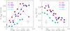 |
Fig. 5 Left: line-of-sight velocity profile of the dense gas within each filament as a function of position form the well centres, i.e. position 8 for Fi-NW (purple dotted line), Fi-SE (red dashed-dotted line), Fi-NEs (blue dashed line), and position 31 for Fi-NEn (cyan solid line). Right: same as left panel but for the total (thermal+non-thermal) dense gas velocity dispersion. |
In the context of longitudinal collapse, the observed velocity gradients are an
indication of the time evolution of each filament as the gradient becomes steeper during
collapse. We can therefore potentially constrain the age of a filament by measuring its
velocity gradient. Pon et al. (2012) showed that
the collapse time of free-falling filaments is  where
τ3D is the spherical free fall time at the same volume
density, and A is the aspect ratio of the filament. This equation shows
that the collapsing time of a filament can be significantly longer than the standard
τ3D. One can compute the time evolution of the filament
velocity gradient as a function of the semi-major axis Z, and this for a
given initial density n0, initial aspect ratio
A0, and initial semi-major axis
Z0, and then compare these to the SDC13 filament observed
values (see Appendix A for more details). Figure 6
shows that the velocity gradients of modelled filaments are consistent with the observed
ones after 1 Myr to 4 Myr of evolution, depending on the projection angles. Similar
collapsing timescales have recently been reported for the massive-star forming filament
NGC 6334 (Zernickel et al. 2013). Also, that Fi-NEn
seems dynamically younger is consistent with the idea that it is collapsing towards a
secondary potential well centre around position 31. Despite the limitations of this
comparison (SDC13 is more of a hub-filament system rather than a single filament – cf.
Fig. 7), these timescales are consistent with the
presence of Class I protostellar sources in the SDC13 filaments.
where
τ3D is the spherical free fall time at the same volume
density, and A is the aspect ratio of the filament. This equation shows
that the collapsing time of a filament can be significantly longer than the standard
τ3D. One can compute the time evolution of the filament
velocity gradient as a function of the semi-major axis Z, and this for a
given initial density n0, initial aspect ratio
A0, and initial semi-major axis
Z0, and then compare these to the SDC13 filament observed
values (see Appendix A for more details). Figure 6
shows that the velocity gradients of modelled filaments are consistent with the observed
ones after 1 Myr to 4 Myr of evolution, depending on the projection angles. Similar
collapsing timescales have recently been reported for the massive-star forming filament
NGC 6334 (Zernickel et al. 2013). Also, that Fi-NEn
seems dynamically younger is consistent with the idea that it is collapsing towards a
secondary potential well centre around position 31. Despite the limitations of this
comparison (SDC13 is more of a hub-filament system rather than a single filament – cf.
Fig. 7), these timescales are consistent with the
presence of Class I protostellar sources in the SDC13 filaments.
4.3. Gravity-driven turbulence and core formation
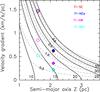 |
Fig. 6 Time evolution of free-falling filaments in the Z − ∇V parameter space. All filaments have the same initial density n0 = 4 × 104 cm-3. Each solid line represents the evolution of a filament with a different initial aspect ratio A0 indicated at the bottom end. Dashed lines represent isochrones from 0.5 Myr to 4 Myr separated by 0.5 Myr. The solid and empty squares mark the positions of the four filaments, for projection angles of 45° and 67°, respectively (cf. text and Appendix A). |
Figure 5 (right) shows the total velocity dispersion (including thermal and non-thermal motions – cf. Arzoumanian et al. 2013) along each filaments. We can see a strong correlation between this quantity and the dense gas velocity, the velocity dispersion increasing towards each of the two centres of collapse (positions 8 and 31). During the collapse of the filaments, the gravitational energy of the gas is converted into kinetic energy (e.g. Peretto et al. 2007; Vázquez-Semadeni et al. 2007). This has been proposed as the main process by which radially collapsing filaments manage to keep a constant width (Arzoumanian et al. 2013). The velocity dispersion resulting from gravitational energy conversion is then a function of the infall velocity and the gas density (Klessen & Hennebelle 2010). The global dynamical evolution of a supercritical filament initially at rest, with uniform density, can be described in two stages (e.g. Peretto et al. 2007). In the first stage, the gas at the filament ends is accelerated more efficiently, and the filament develops a linear velocity gradient increasing from centre to ends. In the second stage, as the matter is accumulated at the centre, the velocity gradient starts to reverse owing to the acceleration close to the central mass becoming larger than at the filament ends. It is clear that in the second stage, both the infall velocity and the velocity dispersion will increase faster at the centre than at the filament ends. However, in the first stage we might expect the infall velocity dispersion and the infall velocity to be greater at the filament ends. In the case of SDC13, the infall velocity is higher at the filament ends, but the velocity dispersion is larger at the centre. This could be explained by the SDC13 filaments being in an intermediate evolutionary stage and/or the initial density profile of SDC13 not being uniform. In fact, SDC13 as a whole has a more complex geometry and density structure than the ones of a single filament, more like a hub-filament system (Myers 2009). In such a configuration, the potential well is dominated by the central mass of the hub. The resulting hub density profile might then favour an early increase in the velocity dispersion during the hub collapse. However, this is speculation and remains to be tested.
The MM1 and MM2 sources, the most massive ones in SDC13, are located near the centre of
the system. Within the context of the free-fall collapse scenario, these sources must have
formed within a tenth of a pc from their current position, suggesting that MM1 and MM2
have basically formed in situ, near the converging point of the filaments. This location
is privileged for source mass growth since flows of dense gas are running towards it, both
bringing more material to be accreted and locally increasing the velocity dispersion. We
can quantify what impact both processes have on core formation. The mass infall rate due
to material running through the filaments can be estimated following
Ṁinf = π(W/2)2ρfilVinf
where W is the filament width, ρfil the
filament density, and Vinf the infall velocity. Using the
average values given in Table 3, along with an
infall velocity Vinf ≃ 0.2 km s-1 at the core
locations, we find that
Ṁinf ≃ 2.5 × 10⁻⁵ M⊙/yr.
This means that over a million years each filament would bring
~25 M⊙ to the SDC13 centre. This is probably an upper limit
since the gas did not fall in for a million years with its current infall velocity. Now,
if we consider that the gravity-driven turbulence acts as a support against gravity, then
the effective Jeans mass becomes  M⊙
(σtot/0.2 km s-1)3.
With a gas velocity dispersion σtot ≃ 0.8 km s-1
towards the centre of the system, the effective Jeans mass goes up to
M⊙
(σtot/0.2 km s-1)3.
With a gas velocity dispersion σtot ≃ 0.8 km s-1
towards the centre of the system, the effective Jeans mass goes up to
 M⊙.
This is close to the observed masses for MM1 and MM2, and it suggests that filament
longitudinal collapse might lead to the formation of super-Jeans cores more as a result of
enhanced turbulent support than as a result of large-scale accretion.
M⊙.
This is close to the observed masses for MM1 and MM2, and it suggests that filament
longitudinal collapse might lead to the formation of super-Jeans cores more as a result of
enhanced turbulent support than as a result of large-scale accretion.
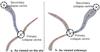 |
Fig. 7 Schematic representation of the the SDC13 velocity field (arrows) a) as viewed on the plane of the sky; b) as viewed sideways with the observer on the left-hand-side of the plot. The two centres of collapse are symbolised by black dashed circles and a cross at their centres. |
5. Conclusion
The presence of protostellar sources and organised velocity gradients along the SDC13 filaments suggest that local and large-scale longitudinal collapse are taking place simultaneously. As a result of the high aspect ratios of the SDC13 filaments, the timescale of the former process is much shorter than for the latter. Here we propose that the large-scale longitudinal collapse mostly contributes to the increase in the turbulent support towards the centre of collapse where starless cores with masses that are an order of magnitude higher than the thermal Jeans mass can form. This study therefore suggests that super-Jeans
prestellar cores may form at the centre of collapsing clouds. Despite this increase in support at the centre of SDC13, the MM1 and MM2 masses are still much lower than the mass of the O-type star-forming core sitting at the centre of SDC335 (Peretto et al. 2013). We speculate that the major difference resides in the mass and morphology of the surrounding gas reservoirs surrounding these sources. Dense, collapsing, spherical clouds of cold gas are more efficient in concentrating matter at their centres in a short amount of time. The study of a larger sample of massive star-forming clouds presenting all sort of morphologies is required to test this assertion.
Online material
Appendix A: Homologous free-fall collapse of filaments
The equation of motion for a filament edge in homologous free-fall collapse is given by
(Pon et al. 2012)
 (A.1)where
Z(t) is the semi-major axis of the filament, and
M its mass. Multiplying each side of Eq. (A.1) by
(A.1)where
Z(t) is the semi-major axis of the filament, and
M its mass. Multiplying each side of Eq. (A.1) by
 and integrating over t, we obtain
![Mathematical equation: \appendix \setcounter{section}{1} \begin{eqnarray} \frac{{\rm d}Z(t)}{{\rm d}t}=V(t)=-\sqrt{2GM[Z(t)^{-1}+\alpha]} \end{eqnarray}](/articles/aa/full_html/2014/01/aa22172-13/aa22172-13-eq150.png) (A.2)where
α is the constant of integration. Now, if we consider a filament
initially at rest, we have V(t = 0) = 0, and therefore
(A.2)where
α is the constant of integration. Now, if we consider a filament
initially at rest, we have V(t = 0) = 0, and therefore
 ,
where Z0 = Z(t = 0) is the
initial semi-major axis of the filament. We can solve for
Z(t) by setting
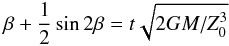
Z(t)/Z0 = cos2β
in Eq. (A.2) and integrating over t again. We then obtain
,
where Z0 = Z(t = 0) is the
initial semi-major axis of the filament. We can solve for
Z(t) by setting
Z(t)/Z0 = cos2β
in Eq. (A.2) and integrating over t again. We then obtain
 (A.3)or,
when replacing the mass by
M = 2πR2Z0ρ0,
(A.3)or,
when replacing the mass by
M = 2πR2Z0ρ0,
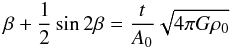 (A.4)where
A0 is the initial aspect ratio of the filament and
ρ0 its initial density. The filament free-fall times
τ1D is calculated for
Z(t)/Z0 = 0,
which means when β = π/2. We
therefore obtain
(A.4)where
A0 is the initial aspect ratio of the filament and
ρ0 its initial density. The filament free-fall times
τ1D is calculated for
Z(t)/Z0 = 0,
which means when β = π/2. We
therefore obtain 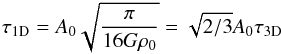 (A.5)where
τ3D is the spherical free-fall time at the same density.
Finally, given that the velocity gradient is linear during the homologous collapse of a
filament, we can compute the velocity gradient
∇V = V(t)/Z(t).
(A.5)where
τ3D is the spherical free-fall time at the same density.
Finally, given that the velocity gradient is linear during the homologous collapse of a
filament, we can compute the velocity gradient
∇V = V(t)/Z(t).
To compute the different values plotted in Fig. 6 we sampled β between 0 and π/2 and used the relevant equations presented in this appendix. We further assumed that the radius of the filaments stays the same during the collapse. For the purpose of the calculations, we took R = 0.15 pc. Figure 6 shows the evolution of seven filaments (solid lines) having all the same initial density n0 = 4 × 104 cm-3 but a different initial aspect ratio5.
Nearly all quantities presented in this paper are affected by projection effect. We can only correct for it if we know the projection angle θ of the filaments with respect to the line of sight. Unfortunately, it is impossible to know the exact value of θ for a given filament. However, for randomly sampled filament orientations one have ⟨ θ ⟩ = 67°. For this letter, we therefore considered two cases, the case where θ = 45° and the case where θ = 67°. The corrected values for the velocity, semi-major axis, and velocity gradients are Vcorr = Vobs/cos(θ), Lcorr = Lobs/sin(θ), and ∇Vcorr = ∇Vobstan(θ). For θ = 45° these corrections meant that the observed velocity gradients remain unaffected, but the semi-major axis becomes larger by a factor 1.4. For θ = 67°, the velocity gradient increases by a factor 2.4 and the semi-major axis by a factor 1.1. The points in Fig. 6 corresponding to the four SDC13 filaments have been corrected by such factors. Much larger angles would lead to very large velocity gradients that have never been observed on parsec scales, while much smaller angles would imply very large initial aspect ratios and semi-major axes. Even though we cannot rule out such configurations, they are unlikely.
Appendix B: Protostellar classes of SDC13 sources
Infrared spectral indexes have been used for more than 20 years to classify YSOs
according to their evolutionary stages. The idea is that the peak of a YSO spectral
energy distribution (SED) evolves from submillimetre to infrared during the first few
million years of its life. Calculating then the slope, i.e. the spectral index, of the
SED at a critical frequency range allows the quantification of this evolution. YSOs
classes are traditionally defined (e.g. Lada &
Wilking 1984; Wilking et al. 1989)
between 2 μm and 10 μm by calculating the following
quantity ![Mathematical equation: \hbox{$\alpha_{[2-10]} = \frac{{\rm d}(\log(\lambda S_{\lambda}))}{{\rm d} (\log(\lambda))}$}](/articles/aa/full_html/2014/01/aa22172-13/aa22172-13-eq177.png) ,
Class I sources having
α[2−10] > 0, Class II sources
0 > α[2−10] > −1.6,
and Class III sources
α[2−10] < −1.6.
,
Class I sources having
α[2−10] > 0, Class II sources
0 > α[2−10] > −1.6,
and Class III sources
α[2−10] < −1.6.
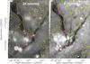 |
Fig. B.1 Left: Spitzer 24 μm image of SDC13 (greyscale) on which we over-plotted the MAMBO 3 mJy/beam contour (yellow). In this image we also report the positions of the seven protostellar sources identified along the SDC13 filaments (purple circles), along with the detection of two extra sources located on the edge of the outer edge of the contour (blue circles). Right: 8 μm image of SDC13 (greyscale). The contour is the same as in the left panel. The purple circles mark the positions of the nine 8 μm sources identified towards the identified 24 μm sources. The meaning of the symbol’s colour is the same as in the left panel. |
In the context of this study we focussed on sources identified at 24 μm. We only considered sources that are spatially coincident with the SDC13 filaments (purple circles in Fig. B.1), limiting potential background/foreground contamination. To extract sources we used the Starfinder algorithm (Diolaiti et al. 2000) and found seven 24 μm sources, five of which have 8 μm counterparts6 (see Fig. B.1). We then calculated their spectral index as estimated between 8 μm and 24 μm (fluxes of multiple 8 μm sources have been combined, and for those with no 8 μm counterpart, we used the 8 μm detection limit of 2 mJy). One advantage provided by these two wavelengths is that they are similarly affected by extinction (Flaherty et al. 2007; Chapman et al. 2009), which implies that estimated values of α[8−24] are not much affected by extinction. As a result, we find three sources with −0.4 < α[8−24] < 0, and another four with 0 < α[8−24] < 2.2. Note that we also report the detection of two additional protostellar sources located on the outer edge of the filament (blue circles in Fig. B.1). Their spectral indexes are ~−1.5, indicating that they might well be background/foreground sources. Note that we do not have any detection towards MM1 at 24 μm. This is because the 24 μm emission is rather diffuse towards this source, and Starfinder failed to find any compact sources, a requirement for protostar detection.
We then used the YSO C2D database of Serpens, Ophiucchi, and Perseus (Evans et al. 2009) to compare the α[2−10] spectral index with α[8−24]. The results of this comparison are displayed in Fig. B.2. Although there is some dispersion and not a one-to-one correlation, there is still a linear correlation between the two indexes. Despite the dispersion in α[8−24], this plot strongly suggests that the seven protostellar sources identified within the SDC13 filaments have mid-infrared spectral indexes consistent with Class I and/or young Class II objects.
We further analysed the properties of the nine 8 μm sources (see Fig. B.1) by constructing a colour-colour diagram using all IRAC Spitzer bands between 3.6 μm and 8 μm. Depending on their colours, sources of different classes are expected to sit in different regions of such diagram (Allen et al. 2004; Megeath et al. 2004). In Fig. B.3 we can see that seven sources sit in the Class I region of the diagram, while the two remaining sources are clearly sitting in the Class III/stellar contamination region. The latter are in fact the two sources located on the edge of the filament (i.e. the blue circles in Fig. B.1), already identified as likely foreground/background sources from our spectral index analysis. Also, extinction can significantly affect the source location in this plot, mostly artificially increasing their [3.6]−[4.5] mag. However, the extracted sources are red enough that even for an extinction of Av = 50, most identified sources would remain in the Class I region of the diagram, the other ones just moving to the other side of the Class II/Class I border. This is consistent with the α[8−24] analysis performed above.
Finally, based on the 24 μm flux of protostellar sources and an assumed extinction, one may obtain an estimate of the source bolometric luminosity (Dunham et al. 2008). Following Parsons et al. (2009) we estimate that, with extinctions in the range of 10 < Av < 50 (matching the range of observed dust column density in SDC13) and 24 μm fluxes between 10 mJy and 60 mJy for all but one source, the SDC13 protostellar sources have bolometric luminosities in the range of 10 L⊙ to few 100 L⊙. Such luminosities stand at the high end of the luminosity distribution of nearby low-mass protostars (Evans et al. 2009), possibly indicating a slightly shorter lifetime of the SDC13 protostellar sources compared to the standard Class I low-mass protostar lifetime.
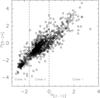 |
Fig. B.2 Mid-infrared spectral indexes for all ~1000 YSOs from the C2D catalogue (Evans et al. 2009). For each source the spectral index has been calculated for two wavelength ranges: from 2 μm to 10 μm and from 8 μm to 24 μm. |
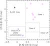 |
Fig. B.3 Mid-infrared [3.6]–[4.5] vs. [5.8]–[8.0] colour–colour diagram for the nine sources extracted at 8 μm. The colour coding is the same as in Fig. B.1. The arrow indicates an extinction of Av = 10. The different regions of the plot corresponding to the different protostellar classes are also shown. |
The sizes are estimated in the same way as for the IRDC catalogue of Peretto & Fuller (2009, see Appendix A), meaning that we calculate the matrix of moment of inertia of the pixels within the 3 mJy/beam contour for each filament. Then we diagonalise the matrix and get two values corresponding to the sizes along the major and minor axes of the filaments. The radius Reff corresponds to the radius of the disc having the same area as the filament. The 3 mJy/beam contour encompasses all filaments, so we artificially divided the MAMBO emission at the filaments junction.
These widths are compatible with the standard 0.1 pc FWHM width observed towards nearby interstellar filaments (Arzoumanian et al. 2011) since the SDC13 measurements we provide here extend beyond the FWHM of the filament profiles.
We observed few core positions in SiO(2–1), well known tracer of protostellar outflows, but did not get any wing emission.
Since we fixed the filament radius, A0 and Z0 are not independent parameters. Also, the aspect ratios given in Table 3 correspond to half of this A0 parameter.
Note that two 24 μm sources split up into two 8 μm sources.
Acknowledgments
We thank the anonymous referee whose report helped improve the quality of this paper. We would like to thank Alvaro Hacar for helping with the MAMBO data reduction. And finally, we want to thank the IRAM 30 m staff for their support during the observing runs. N.P. was partly supported by a CEA/Marie Curie Eurotalents fellowship and benefited from the support of the European Research Council advanced grant ORISTARS (Grant Agreement No. 291294).
References
- Allen, L. E., Calvet, N., D’Alessio, P., et al. 2004, ApJS, 154, 363 [NASA ADS] [CrossRef] [Google Scholar]
- André, P., Men’shchikov, A., Bontemps, S., et al. 2010, A&A, 518, L102 [NASA ADS] [CrossRef] [EDP Sciences] [Google Scholar]
- Arzoumanian, D., André, P., Didelon, P., et al. 2011, A&A, 529, L6 [Google Scholar]
- Arzoumanian, D., André, P., Peretto, N., & Könyves, V. 2013, A&A, 553, A119 [NASA ADS] [CrossRef] [EDP Sciences] [Google Scholar]
- Busquet, G., Zhang, Q., Palau, A., et al. 2013, ApJ, 764, L26 [NASA ADS] [CrossRef] [Google Scholar]
- Carey, S. J., Noriega-Crespo, A., Mizuno, D. R., et al. 2009, PASP, 121, 76 [NASA ADS] [CrossRef] [Google Scholar]
- Chapman, N. L., Mundy, L. G., Lai, S.-P., & Evans, N. J. 2009, ApJ, 690, 496 [NASA ADS] [CrossRef] [Google Scholar]
- Churchwell, E., Babler, B. L., Meade, M. R., et al. 2009, PASP, 121, 213 [NASA ADS] [CrossRef] [Google Scholar]
- Diolaiti, E., Bendinelli, O., Bonaccini, D., et al. 2000, A&AS, 147, 335 [NASA ADS] [CrossRef] [EDP Sciences] [Google Scholar]
- Duarte-Cabral, A., Fuller, G. A., Peretto, N., et al. 2010, A&A, 519, A27 [NASA ADS] [CrossRef] [EDP Sciences] [Google Scholar]
- Dunham, M. M., Crapsi, A., Evans, II, N. J., et al. 2008, ApJS, 179, 249 [NASA ADS] [CrossRef] [Google Scholar]
- Evans, N. J., Dunham, M. M., Jørgensen, J. K., et al. 2009, ApJS, 181, 321 [NASA ADS] [CrossRef] [Google Scholar]
- Flaherty, K. M., Pipher, J. L., Megeath, S. T., et al. 2007, ApJ, 663, 1069 [CrossRef] [Google Scholar]
- Hacar, A., & Tafalla, M. 2011, A&A, 533, A34 [NASA ADS] [CrossRef] [EDP Sciences] [Google Scholar]
- Henshaw, J. D., Caselli, P., Fontani, F., et al. 2013, MNRAS, 428, 3425 [NASA ADS] [CrossRef] [Google Scholar]
- Kirk, J. M., Ward-Thompson, D., & André, P. 2005, MNRAS, 360, 1506 [NASA ADS] [CrossRef] [Google Scholar]
- Kirk, H., Myers, P. C., Bourke, T. L., et al. 2013, ApJ, 766, 115 [NASA ADS] [CrossRef] [Google Scholar]
- Klessen, R. S., & Hennebelle, P. 2010, A&A, 520, A17 [NASA ADS] [CrossRef] [EDP Sciences] [Google Scholar]
- Lada, C. J., & Wilking, B. A. 1984, ApJ, 287, 610 [NASA ADS] [CrossRef] [Google Scholar]
- Megeath, S. T., Allen, L. E., Gutermuth, R. A., et al. 2004, ApJS, 154, 367 [NASA ADS] [CrossRef] [Google Scholar]
- Miettinen, O. 2012, A&A, 540, A104 [NASA ADS] [CrossRef] [EDP Sciences] [Google Scholar]
- Molinari, S., Swinyard, B., Bally, J., et al. 2010, A&A, 518, L100 [NASA ADS] [CrossRef] [EDP Sciences] [Google Scholar]
- Myers, P. C. 2005, ApJ, 623, 280 [NASA ADS] [CrossRef] [Google Scholar]
- Myers, P. C. 2009, ApJ, 700, 1609 [NASA ADS] [CrossRef] [EDP Sciences] [Google Scholar]
- Ostriker, J. 1964, ApJ, 140, 1056 [NASA ADS] [CrossRef] [MathSciNet] [Google Scholar]
- Parsons, H., Thompson, M. A., & Chrysostomou, A. 2009, MNRAS, 399, 1506 [NASA ADS] [CrossRef] [Google Scholar]
- Peretto, N., & Fuller, G. A. 2009, A&A, 505, 405 [NASA ADS] [CrossRef] [EDP Sciences] [Google Scholar]
- Peretto, N., & Fuller, G. A. 2010, ApJ, 723, 555 [NASA ADS] [CrossRef] [Google Scholar]
- Peretto, N., Hennebelle, P., & André, P. 2007, A&A, 464, 983 [NASA ADS] [CrossRef] [EDP Sciences] [Google Scholar]
- Peretto, N., Fuller, G. A., Plume, R., et al. 2010, A&A, 518, L98 [NASA ADS] [CrossRef] [EDP Sciences] [Google Scholar]
- Peretto, N., Fuller, G. A., Duarte-Cabral, A., et al. 2013, A&A, 555, A112 [NASA ADS] [CrossRef] [EDP Sciences] [Google Scholar]
- Pon, A., Johnstone, D., & Heitsch, F. 2011, ApJ, 740, 88 [NASA ADS] [CrossRef] [Google Scholar]
- Pon, A., Toalá, J. A., Johnstone, D., et al. 2012, ApJ, 756, 145 [NASA ADS] [CrossRef] [Google Scholar]
- Ragan, S. E., Heitsch, F., Bergin, E. A., & Wilner, D. 2012, ApJ, 746, 174 [NASA ADS] [CrossRef] [Google Scholar]
- Reid, M. J., Menten, K. M., Zheng, X. W., et al. 2009, ApJ, 700, 137 [NASA ADS] [CrossRef] [Google Scholar]
- Rosolowsky, E. W., Pineda, J. E., Kauffmann, J., & Goodman, A. A. 2008, ApJ, 679, 1338 [NASA ADS] [CrossRef] [Google Scholar]
- Sadavoy, S. I., Di Francesco, J., & Johnstone, D. 2010, ApJ, 718, L32 [NASA ADS] [CrossRef] [Google Scholar]
- Vázquez-Semadeni, E., Gómez, G. C., Jappsen, A. K., et al. 2007, ApJ, 657, 870 [NASA ADS] [CrossRef] [Google Scholar]
- Wilking, B. A., Lada, C. J., & Young, E. T. 1989, ApJ, 340, 823 [NASA ADS] [CrossRef] [Google Scholar]
- Zernickel, A., Schilke, P., & Smith, R. J. 2013, A&A, 554, L2 [NASA ADS] [CrossRef] [EDP Sciences] [Google Scholar]
All Tables
All Figures
|
Fig. 1 Spitzer 8 μm image of SDC13 in grey scale on top of which we overlaid the IRAM 30 m MAMBO 1.2 mm dust continuum contours (from 3 mJy/beam to 88 mJy/beam in step of 5 mJy/beam). The positions of the identified 1.2 mm compact sources within the SDC13 filaments are marked as crosses, red for starless sources and blue for protostellar sources. |
| In the text | |
|
Fig. 2 Left: Spitzer 8 μm image of
SDC13 in grey scale on top of which we marked the 31 single-pointing positions we
observed in N2H+(1–0), and the skeletons of each filament
(thick solid lines). The size of the black circles represents the 30 m beam size at
3.2 mm. Right: examples of three N2H+(1–0)
spectra (displayed on |
| In the text | |
|
Fig. 4 Spitzer 8 μm image of SDC13 in grey scale on top of which we symbolised the results of the N2H+(1–0) HFS fitting as circles. The colour of the symbols indicate the gas velocity while their sizes indicate the gas velocity dispersion (FWHM). |
| In the text | |
|
Fig. 5 Left: line-of-sight velocity profile of the dense gas within each filament as a function of position form the well centres, i.e. position 8 for Fi-NW (purple dotted line), Fi-SE (red dashed-dotted line), Fi-NEs (blue dashed line), and position 31 for Fi-NEn (cyan solid line). Right: same as left panel but for the total (thermal+non-thermal) dense gas velocity dispersion. |
| In the text | |
|
Fig. 6 Time evolution of free-falling filaments in the Z − ∇V parameter space. All filaments have the same initial density n0 = 4 × 104 cm-3. Each solid line represents the evolution of a filament with a different initial aspect ratio A0 indicated at the bottom end. Dashed lines represent isochrones from 0.5 Myr to 4 Myr separated by 0.5 Myr. The solid and empty squares mark the positions of the four filaments, for projection angles of 45° and 67°, respectively (cf. text and Appendix A). |
| In the text | |
|
Fig. 7 Schematic representation of the the SDC13 velocity field (arrows) a) as viewed on the plane of the sky; b) as viewed sideways with the observer on the left-hand-side of the plot. The two centres of collapse are symbolised by black dashed circles and a cross at their centres. |
| In the text | |
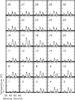 |
Fig. 3 N2H+(1–0) spectra observed for each position along the SDC13 filaments (see Fig. 2). |
| In the text | |
|
Fig. B.1 Left: Spitzer 24 μm image of SDC13 (greyscale) on which we over-plotted the MAMBO 3 mJy/beam contour (yellow). In this image we also report the positions of the seven protostellar sources identified along the SDC13 filaments (purple circles), along with the detection of two extra sources located on the edge of the outer edge of the contour (blue circles). Right: 8 μm image of SDC13 (greyscale). The contour is the same as in the left panel. The purple circles mark the positions of the nine 8 μm sources identified towards the identified 24 μm sources. The meaning of the symbol’s colour is the same as in the left panel. |
| In the text | |
|
Fig. B.2 Mid-infrared spectral indexes for all ~1000 YSOs from the C2D catalogue (Evans et al. 2009). For each source the spectral index has been calculated for two wavelength ranges: from 2 μm to 10 μm and from 8 μm to 24 μm. |
| In the text | |
|
Fig. B.3 Mid-infrared [3.6]–[4.5] vs. [5.8]–[8.0] colour–colour diagram for the nine sources extracted at 8 μm. The colour coding is the same as in Fig. B.1. The arrow indicates an extinction of Av = 10. The different regions of the plot corresponding to the different protostellar classes are also shown. |
| In the text | |
Current usage metrics show cumulative count of Article Views (full-text article views including HTML views, PDF and ePub downloads, according to the available data) and Abstracts Views on Vision4Press platform.
Data correspond to usage on the plateform after 2015. The current usage metrics is available 48-96 hours after online publication and is updated daily on week days.
Initial download of the metrics may take a while.