| Issue |
A&A
Volume 561, January 2014
|
|
|---|---|---|
| Article Number | A145 | |
| Number of page(s) | 11 | |
| Section | Interstellar and circumstellar matter | |
| DOI | https://doi.org/10.1051/0004-6361/201321946 | |
| Published online | 27 January 2014 | |
New light on the multiple jets of CRL 618
1 Departament de Física i Enginyeria Nuclear, EUETIBUniversitat Politécnica de Catalunya Comte d’Urgell 187 08036 Barcelona Spain
e-mail: angels.riera@upc.edu; [angels.riera;arjuna.castrillon]@upc.edu
2 Departament d’Astronomia i Meteorologia, Universitat de Barcelona, 08028 Barcelona, Spain
3 Instituto de Ciencias Nucleares, Universidad Nacional Autónoma de México, CP: 04510 México D.F., Mexico
e-mail: pablo@nucleares.unam.mx; Raga@nucleares.unam.mx
Received: 23 May 2013
Accepted: 26 November 2013
Context. Proto-planetary nebulae (pPNe) are thought to represent the transitory phase of the late stages of low- to intermediate-mass stars. Most pPNe show a bipolar or multipolar geometry. The process(es) that transforms the spherical asymptotic giant branch (AGB) ejecta into a bipolar/multipolar geometry is not known in detail. Interactions between stars in a binary system are suspected to cause the departure from spherical symmetry.
Aims. We aim to determine whether the existence of a binary source that ejects a wind (from the primary) and a bipolar precessing jet with a time-dependent ejection velocity (from the orbiting companion) could produce the morphology and kinematics of the well-known multipolar pPN CRL 618.
Methods. We applied an anisotropic wavelet analysis to the [S ii] Hubble Space Telescope (HST) images of CRL 618 to determine the charateristic sizes of various small-scale structures across and along the optical jets of CRL 618. From the archival [S ii] HST images of CRL 618 with a 10.7 yr time base, we carried out proper-motion measurements of the emission structures observed in the lobes of CRL 618. We computed six 3D numerical simulations of a precessing, time-dependent ejection velocity jet launched from a hypothetical companion star of a binary system.
Results. We found the proper motions to be well aligned with the jet axis with tangential velocities ranging from 60 to 430 km s-1. The tangential velocity is a monotonically increasing function of the distance to the central source. We found that our numerical simulations reproduce the morphology and proper-motion measurements of CRL 618 when we considered a trend of decreasing jet velocity with time to reproduce the tangential velocity vs. distance dependence.
Conclusions. From the comparison we made between the structure and proper motions observed in CRL 618 and predictions from 3D jet simulations, we found that the size and morphology of the lobes and the proper motion behavior of CRL 618 can be explained in terms of a well-collimated bipolar ejection, a precession of the outflow axis, an approximately periodic time-variability of the outflow velocity (with a period of ~15 yr), and a long-term trend of decreasing outflow velocities from dynamical timescales of 50 yr towards more recent times.
Key words: ISM: jets and outflows / planetary nebulae: individual: CRL 618
© ESO, 2014
1. Introduction
CRL 618 was identified as an object in transition from the asymptotic giant branch (AGB) to a planetary nebula (PN), that is in the proto-planetary nebula (pPN) phase, based on its optical, infrared and radio properties (Westerbrook et al. 1975). Ground-based optical and near-infrared imaging of CRL 618 revealed two lobes of emission separated by a dark lane. Hubble Space Telescope (HST) narrowband images revealed highly collimated outflows (or jets) showing a multipolar geometry (Trammell & Goodrich 2002). These jets are known to have high velocities in the optical lines (Carsenty & Solf 1982; and Sánchez Contreras et al. 2002). High velocities and multipolar jets are also seen in molecular gas. High-velocity features associated with the optical jets, with velocities up to 200 km s-1, were detected in H2 (Cox et al. 2003). Dense molecular gas detected in CO is also outflowing at velocities on the order of 200 km s-1 (Cernicharo et al. 1989; Sánchez Contreras et al. 2004; Bujarrabal et al. 2010; Soria-Ruiz et al. 2013). Recent interferometric maps of the CO J = 1−2 emission showed different molecular components in CRL 618: 1) a compact bipolar outflow (at a velocity higher than 200 km s-1); 2) large expanding torus (~11′′) perpendicular to the outflow; 3) a compact dense torus-like core perpendicular to the outflow; and 4) an extended round halo (Sánchez Contreras et al. 2004; Sánchez Contreras & Sahai 2004; Lee et al. 2013).
Surrounding the central star, there is a compact H II region elongated in the east-west direction, detected in the centimeter and millimeter-wave continuum (Kwok & Feldman 1981; Kwok & Bignell 1984; Martín-Pintado et al. 1988). This elliptical H II region has increased in flux and size over a period of ~26 years (Tafoya et al. 2013).
Recently, proper-motion measurements of the outermost features of the jets of CRL 618 have been obtained from Hα HST images with a time base of 11 years (Balick et al. 2013). Balick et al. reported tangential velocities of ~300 km s-1.
HST [S ii] images of CRL 618.
From early ground-based observations, the optical emission from the lobes has been known to be shock-excited (Trammell et al. 1993; Sánchez Contreras et al. 2002; Riera et al. 2006). More recently, Riera et al. (2011) have analyzed the HST STIS spectra of several features of the jets of CRL 618 with unprecedented spatial resolution. Unfortunately, the slit was displaced from the leading bow-shocks. Comparing the observations with plane-parallel shock models, Riera et al. (2011) found that the shock velocities lie in a narrow range between 30 and 40 km s-1, except for the [O iii]/Hβ line ratios which require higher shock velocities (80–90 km s-1). The predicted shock velocities are significantly lower than the velocities with which the jets move outward.
Several models have been invoked to explain the bipolar/multipolar morphology of some pPNe. Most are based on the presence of a bipolar jet or collimated fast wind (CFW) ejected by one of the stars in a binary system (e.g., Morris 1987; Soker & Rappaport 2000). Hydrodynamical simulations with a time dependent ejection velocity and/or precessing jets have successfully reproduced the morphology of bipolar pPNe and PNe, such as the point-symmetric nebulae: Hen 3-1475 (Velázquez et al. 2004), PN K 3−35 (Velázquez et al. 2007), IC 4634 (Guerrero et al. 2008), and the Red Rectangle (Velázquez et al. 2011). In particular, there are some numerical simulations that try to reproduce the morphology and kinematics of CRL 618, such as the study of Lee & Sahai (2003), who proposed that the CFW interacts with a spherical AGB wind (see also, Lee et al. 2009); alternatively, Dennis et al. (2008) proposed that the multiple jet appearance of CRL 618 could be due to clumps moving outwards at high velocities and slightly different directions. Balick et al. (2013) have explored the nature of the jets of CRL 618 by means of 3D hydrodynamical simulations of either a bullet or a continuous jet moving through the remnant AGB wind. These authors favored the “bullet” hypothesis based on the multipolar morphology.
Some studies have been carried out to explain how both mirror- and point-symmetric morphologies can be obtained from a precessing jet from a binary system (see, e.g., Raga et al. 2009). Haro-Corzo et al. (2009) analyzed the influence of the orbital motion on the optical emission of these objects, by means of 3D hydrodynamical simulations. Their predicted [N ii] emission line maps can produce different luminosities for the two lobes, as observed in CRL 618 (Sánchez Contreras et al. 2002; Riera et al. 2011).
More recently, Velázquez et al. (2012, 2013) have shown that the existence of a binary source that ejects a wind (from the primary star) and a bipolar, precessing jet with time-dependent ejection velocity (from the orbiting companion) can reproduce the multipolar geometry of pPNe. These authors have shown that the large-scale morphological characteristics of these nebulae (lobe size, semi-aperture angle, number of observed lobes) can be related to some of the parameters of the binary system.
Two sets of HST images taken with a time interval of 10.7 years are used in this paper to study the morphology and the proper motions of the jets of CRL 618. The paper is organized as follows, the observations are described in Sect. 2. In Sect. 3 we describe the wavelet technique and the procedure we applied to calculate the proper motion of the emission features of the jets of CRL 618. The results are shown in Sect. 4. We compute numerical simulations of a precessing jet with a variable ejection velocity ejected by the secondary star of a binary system, which are compared with the [S ii] HST images (Sect. 5). Finally, we summarize our results in Sect. 6.
2. Observations
The images used in this paper to determine the proper motion of the jets of CRL 618 were retrieved from the HST Data Archive1. Two data sets of CRL 618 were obtained with the HST through some narrowband filters. The first set of images was taken on 1998 November 23 with the Wide Field Planetary Camera 2 (WFPC2) (GO 6761, PI: Trammell), and three narrowband filters selected to isolate the [S ii] 6716, 6731 Å emission lines (F673N), the [O I] 6300 Å emission line (F631N), and the Hα emission (F656N). The second data set was obtained with the Wide Field Camera 3 (WFC3) on 2009 August 8 (GO 11580, PI: Balick) through three narrowband filters isolating the Hα emission (F656N), the [N ii] 6584 Å emission line (F658N), and the [S ii] 6716, 6731 Å emission lines (F673N). Among the four narrowband filters used, the F673N and F656N are in common in both sets. Note that the Hα (F656N) images have two components: the emission formed in the lobes and the scattered component (Hα emission scattered by the dust outflow) (Carsenty & Solf 1982; Riera et al. 2011). We measured the proper motion of the bow-shaped and knotty features from the two [S ii] images, which proved to be the most suitable because the observed emission arises from the jets. Although the filter names remainded the same in both sets, their characteristics have changed (see Table 1). Table 1 presents the details of the two observations.
The first images of CRL 618 were obtained as part of the HST Cycle 6 program 6761. CRL 618 was at the center of the planetary camera which has a field of view of 36″ × 36″ and a plate scale of 0 045 pixel-1. The images were reduced through the HST WFPC2 data reduction pipeline (for a detailed description of the data reduction see Trammell & Goodrich 2002). The second set of images was obtained as part of cycle 17 (GO 11580, PI: Balick) with the WFC3 ultraviolet and visible channel (UVIS) camera, which has a 20″ × 20″ field of view and a plate scale of 00395 pixel-1 (Balick et al. 2013).
The analysis started with the pipeline-reduced data products provided by the Hubble archive. The two-epoch [S ii] 6716 + 6731 Å images were converted into a common reference system and rebinned to the same pixel scale (0045 pixel-1). The determination of accurate proper motions requires the multiepoch images to be registered to subpixel accuracy. When the observed field contains many background stars, image registration is easy to implement and the distortions introduced by the optical system can be corrected for. However, in the case of the two [S ii]-images of CRL 618 only one field star was detected in both exposures. The images were initially aligned using the absolute astrometry as returned by the pipeline reduction. Then both images were rebinned to the same pixel scale (0045 pixel-1) and aligned using the field star and the small structure seen in the innermost part of the east lobe (labeled A′ in Fig. 1, see also Sánchez Contreras et al. 2002), which has a spectrum different from that of the lobes. Sánchez Contreras et al. (2002) proposed that this region is ionized by the UV stellar radiation and that it corresponds to the outermost parts of the H II region surrounding the star. Balick et al. (2013) proposed that A′ (visible in several optical and NIR images) is the central exciting source of CRL 618. We assumed that A′ is a stationary feature that was used to align the two [S ii] images. The proper-motion measurements obtained with this assumption are along the jet axes (as expected), and the tangential velocity values therefore are consistent with the proper motions displayed by outflows of PNe (such as Hu 1–2, Miranda et al. 2012).
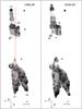 |
Fig. 1 CRL 618 in the 1998.89 (left) and 2009.60 (right) [S ii] images shown to the same scale and pixel size (0 |
The images were aligned and rotated using the standard IRAF routines GEOMAP and GEOTRAN. The accuracy of the relative alignment between the two images is approximately 0.5 pixels (i.e., ≤ ).
).
3. Analysis
The [S ii] HST images of CRL 618 show at least four different jets in its lobes (see Fig. 1). We named these four jets J1, J2 (in the bright eastern lobe), and J1′ and J2′ in the faint lobe (as indicated in Fig. 1).
3.1. Small-scale structure: wavelet technique
The [S ii] images of CRL 618 show the complex structure of its jets, with knots, arc-shaped structures, and diffuse emission. A comparison between the two epochs indicates remarkable morphological changes. Because of the complexity of the observed jets, we carried out an analysis based on wavelet transforms, which allow us to obtain a general description of the flow.
The wavelet transform decomposes an image into maps of different scales. In each map, structures with the chosen scales are prominent because they have higher coefficients than those with smaller or larger scales. Wavelet transforms have been used in different astrophysical contexts. For example, Grosdidier et al. (2001) used 2D wavelets to isolate stochastic structures of different characteristic sizes in M 1-67 from its Hα image; Riera et al. (2003) studied the complex spatial structure of knots in HH 110 using the wavelet technique. In this paper, we are interested in identifying the characteristics of the complex spatial structure of the lobes of CRL 618 without loosing the positional information. This study shares many similarities with the study of the characteristic sizes of knots along HH 110. Therefore, we adopted the procedure developed by Riera et al. (2003).
The two-dimensional wavelet transform analysis is used to obtain the position of the features of its lobes. We rotated the images of each jet so that the jet axis is parallel to the ordinate. The jet axes are shown in Fig. 1. On these rotated images, we carried out a decomposition on a basis of anisotropic wavelets, which have different sizes along and across the radial (axial) direction. Following Riera et al. (2003), we used a basis of “Mexican hat” wavelets of the form  (1)where r = [(x/ax)2 + (y/ay)2] 1/2],
  , and ax and ay are the scale lengths of the wavelet along the x- and y-axes respectively. Following Riera et al. (2003), we chose a range for ax and ay, which were taken to have integer values from 1 to 60 pixels (i.e., from
  to
to  ), and we then compute the convolutions
  (2)where r′ = [ [(x′ − x)/ax] 2 + [(y′ − y)/ay] 2] 1/2, and I(x,y) is the observed emission map as a function of position (x,y). These convolutions are calculated with a standard FFT algorithm.
We computed the transform maps Tax,ay(x,y) for the [S ii] images for each jet at the two epochs. The convolved maps were used as follows. First, we fixed the position of y on the observed intensity map and found the values of xk (k = 1,2,3) where the intensity map has a local maximum. For each pair (xk,y) where I(x,y) has a maximum, we determined (ax,k,ay,k) in the ax and ay-space where wavelet transform has a local maximum. In this way, we detected the characteristic size of a feature with an intensity maximum at (xk,y).
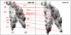 |
Fig. 2 Bright (east) lobe in the 1998.89 (left) and 2009.60 (right) [S ii] images. Several features along regions J1 and J2 are marked and labeled. Changes in the structure of the labeled features between both epochs are discussed in the text. The red arrows show the assumed identifications of corresponding knot pairs in the two epochs. |
The results obtained with the process described above are shown in Figs. 4 and 5. Figures 4 and 5 show the characteristic sizes of the small structures of the bright lobe (Fig. 4) and the faint lobe (Fig. 5) as a function of position along each jet axis.
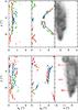 |
Fig. 4 First-epoch [S ii] image of the J1 (bottom) and J2 (top) jets and the characteristic sizes of the small-scale features observed in the optical lobes (ax,k (left) and ay,k (right)) as a function of position y along the jet axis, obtained from the wavelet analysis. The k = 1 peaks are represented in red, k = 2 in green, and k = 3 in blue. Three examples of the compact knots (K), arc, and leading bow-shock (BS) classes are labeled. |
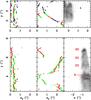 |
Fig. 5 Same as Fig. 4, but for the faint lobe. The J1′ jet is presented in the bottom panel. The J2′ jet is shown in the top panel. Three examples of the compact knots (K), elongated structures (ES), and leading bow-shock (BS) classes are labeled. |
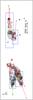 |
Fig. 6 Proper motions of the individual features in the jets of CRL 618. First-epoch [S ii] image of CRL 618 together with the boxes in which the cross-correlations were made (see text). The red boxes correspond to individual knots. Features that include more than one knot (as E1, E9 and W3) are marked in green. The blue boxes were used to measure the proper motion of the J1, J2, J1′ and J2′ jets. The arrows show the computed proper motions. The length of each arrow is proportional to the proper motion. The vertical arrow at the top right shows a proper motion of 300 km s-1. |
3.2. Proper-motion measurements
The first- and second-epoch F673N images used for the proper-motion measurements were converted into a common reference system and rotated so that the y-axis lay along the bipolar axis. The resulting images are shown in Figs. 1, 2 and 3, which also show the assumed identifications of corresponding feature pairs in the two epochs. Strong changes in morphology occur over this time period. These structural changes add uncertainties to the proper-motion measurements and in a few cases even prevent their determination.
Several features within the lobes of CRL 618 exhibit significant morphological changes in the 10.7 years that passed between the two epochs. Knot E3 was a bright feature in the 1998.89 image but in the second epoch (2009.60) it faded and changed from an arc-shaped morphology to being stretched – and more diffuse – along the jet axis. Knot E4 also faded over this time period. These changes made reliable proper motion measurements for E3 and E4 impossible. Although structure E9 (a/b/c) has varied significantly in morphology over the time period, we computed the proper motion of each knot (i.e., features E9a, E9b and E9c) and the proper motion of the whole structure.
In Fig. 1 one can see that some of the features show clear proper motions. We computed the two-dimensional cross-correlation function of the emission detected within previously defined boxes containing the emission features under study (Fig. 2). We also defined four boxes (shown in Fig. 6) including the J1, J2, J1′ and J2′ emission regions. Finally, the proper motions were determined through a parabolic fit to the peak of the cross-correlation (see Reipurth et al. 1992; and López et al. 1996 for a description of this method). The uncertainty in the position of the correlation peak was estimated through the scatter of the correlation peak positions obtained from boxes different from the nominal one in 0 or ±2 pixels (or 0090) in any of its four sides. The error adopted includes the uncertainty in the relative alignment between the two images (≤003) and the uncertainty in the position of the correlation peak. The uncertainty in the identification of corresponding knot pairs are not included in the errors quoted in Table 6. The numerical results are presented in Table 2, which includes the derived proper motions (in milliarcsec yr-1), the tangential velocities (in km s-1) for an adopted distance of 1 kpc (Goodrich 1991; Sánchez Contreras et al. 2004), and the position angle of the proper-motion vectors.
4. Results
4.1. Small-scale structure
The results obtained with the wavelet analysis are shown in Figs. 4 and 5. The distances are measured from A′.
Figure 4 shows ax,k and ay,k (k = 1,2,3) as a function of position (y) along the jet for the two jets identified in the bright (east) lobe. We describe the charateristic sizes of the small-scale structures along J1 to explore the information that can be extracted from the wavelet technique. At  (i.e., at knot E6) the width ranges from
  to
to  and the size along feature E6 shows a V-shaped feature with a decrease toward the intensity peak and then increases up to
  toward the east. At larger y (from
  to
to  ) the structures become elongated with a more or less constant value of
  (i.e., a projected size of 3.0× 1016 cm at the adopted distance). At the arc including E4, ay,k remains constant (~
 –
– ) and the charateristic width ranges from ~
 to . At
  to
to  (i.e., the arc delimited by knots E2 and E3) we see a transition from structures which are elongated along the jet axis to knotty/clumpy features charaterized by widths from
  up to
up to  , and ay,k either lower than 0
 or higher than 1
 . Finally, knot E1 and its tail (at y distances from
  to
to  ) show a V-shaped feature in the ay,k vs. y plot, with values from ~ at the tail to ≤
 (i.e. unresolved) at the intensity peak, while the ax,k values range from to .
Both jets (J1 and J2) show elongated structures with similar values at the central region of each jet ( to
to  ). In Fig. 4 we can compare the overall behavior of the width across the outflows J1 and J2 as a function of distance along the jet axis (ax,k vs. y). Along J1, ax,k decreases more or less monotonically from ~1 at E6 to 0″.2 at E1 (i.e., along 3″). We deduce that the J1 outflow narrows with the distance to the central source with a half-opening angle ~15°. J2 shows a more or less constant width (with an ax,k mean value of 0
 ) for y distances up to 6 and a significantly lower value (≤0
 ) at E7. J2 is more clumpy, showing a larger number of compact knots (detected as V-shaped features in the ay,k vs. y plot).
Proper motions of identified features.
A similar analysis was applied to all jets (i.e. J1, J2, J1′ and J2′). We searched for patterns in the appearance of the small-scale features based on the size across and along the jet axis. We considered morphological classes: knots (either compact knots and leading bow-shocks), elongated (along the jets axis) features, and elongated and wide arcs. The compact-knot class is composed of features that show low values of ax,k and ay,k as W3a, W3b and E11. The compact knots have sizes ~ 6 × 1015 cm along and across the jet axis. The leading bow-shocks (E1, E7, W1b) have widths ranging from 1.5 × 1015 cm to ≤1016 cm, while the charateristic sizes along the flow are ≤1.2 × 1016 cm. The elongated features include W1a, W2 and E10, having ax,k ≤6 × 1015 cm and ay,k ≥ 3 × 1016 cm. The elongated and wide arc class includes the E4 arc and the E2+E3 arc, which have ax,k ≤ 1.5 × 1016 cm and ay,k ≃ 1.5 to 3 × 1016 cm.
4.2. Proper-motion measurements
Figure 6 shows the proper-motion measurements obtained through the process described in Sect. 3.2. The resulting tangential velocities (for a distance of 1kpc toward CRL 618) and the position angles are given in Table 2. The J1′ and J2′ jets (west lobe) have velocities with moduli ~120 km s-1 and approximately along the jet axes. The proper motions we obtained for the outer knots of CRL 618 are roughly consistent with the proper motions of ~300 km s-1 reported by Balick et al. (2013). Balick et al. (2013) extracted their results from a pair of F606W images obtained from the ACS in 2002.6 and WFC3 in 2009.6. These authors determined the overall expansion of the outer bow-shocks by applying a magnification factor to the first image.
All the knots show proper motions in the direction of the corresponding jet axis (either the J1, J2, J1′ or the J2′ jet axes), with the exception of knot E6. As can be seen, there are strong velocity variations along the jets, with tangential velocities ranging from 60 km s-1 to 430 km s-1. In Fig. 7, we show the tangential velocities as a function of distance d to the feature A′. As is clear from this figure, the tangential velocities rapidly increase for increasing distances from the central source. The outer (bow-shock-like) knots show the highest proper-motion values, from 245 up to 430 km s-1. We find the largest proper motion measurement at knot E7 (i.e., the leading bow shock-feature of the J2 jet), which shows a value ~430 km s-1. Large proper motions were also measured in the leading bow-shocks of J1′ and J2′ (W1a/b, W4b) with a mean value ~370 km s-1. Finally, knots E1 and E8 have tangential velocities that are significantly lower than the values reported above (i.e., 288 and 245 km s-1 respectively). The innermost knots (i.e., E5, E6, W5 and W2) have the lowest tangential velocities with values ≤100 km s-1. Several knots at  to show intermediate velocity values, which range from 100 to 200 km s-1.
We calculated the kinematic age (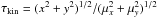 ) of the outermost bow shock-like knots. Knots E1 and E7 have a kinematic age of ~100 years. The W1b and W4b have kinematical ages that are younger (~85 years (W1b) and 50 years (W4b)). These values agree with the age of ~100 yr reported by Balick et al. (2013).
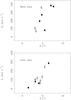 |
Fig. 7 Tangential velocity as a function of distance to the central H II region. Top panel: faint lobe (J1′ (circles), J2′ (squares)). Bottom panel: bright lobe (J1 (circles), J2 (squares)). |
5. Numerical simulations
5.1. Code description and initial setup
We calculated 3D numerical simulations with the Yguazú-a hydrodynamical code (Raga et al. 2000), which integrates the gasdynamical equations with a second-order accurate scheme (in time and space) using the “flux-vector splitting” method of van Leer (1982) on a binary adaptive grid. Together with the gas-dynamic equations, several rate equations for atomic/ionic species were also integrated. These species are H i, H ii, He i, He ii, He iii, [C ii], [C iii], [C iv], [N i], [N ii], [N iii], [O i], [O ii], [O iii], [O iv], [S ii], and [S iii] (see details of the reaction and cooling rates in Raga et al. 2002). These rate equations enable the computation of a nonequilibrium cooling function. Considering the temperature and density distributions obtained from the numerical simulations, we can compute the [S ii]λλ 6716, 6730 emission coefficients. The intensities of the forbidden lines [S ii]λλ 6716, 6730 were calculated by solving five-level atom problems, using the parameters of Mendoza (1983). These intensities can be integrated along the line of sight to produce synthetic emission maps.
A computational domain of (1.5, 1.5, 3) × 1017 cm along the x-, y-, and z-axes, respectively, was employed. These sizes correspond to the observed angular size for a distance of 1 kpc. An adaptive Cartesian grid with five refinement levels was used, achieving a resolution of ~5.9 × 1014 cm (~0040 at a distance of 1 kpc) at the finest level, corresponding to (256 × 256 × 512) pixels in a uniform grid.
Following the work of Velázquez et al. (2012; see also Velázquez et al. 2013), we considered a precessing and a time-dependent ejection velocity jet, that is launched from the companion star of a binary system. This jet propagates into a dense and slow wind of the AGB primary star. At the initial time (and filling the whole computational domain), we imposed an isotropic, constant velocity AGB wind with a density distribution, that considers the final superwind phase of the AGB star (Mellema 1995), given by: ![\begin{equation} \rho_{\rm w}=\frac{1}{2}\left[(\rho_{\rm sup}+\rho_{\rm AGB})+(\rho_{\rm sup}-\rho_{\rm AGB}) \cos\epsilon\right] \left(\frac{r_{\rm w}}{r}\right)^2, \label{rhoagb} \end{equation}](/articles/aa/full_html/2014/01/aa21946-13/aa21946-13-eq91.png) (3)which is:
(3)which is: ![\begin{equation} \epsilon=\pi \min\left[1,\max\left[0,\ \frac{r-(r_{\rm w}+v_{\rm w} t_{\rm sup})}{v_{\rm w} t_{\rm trans}}\right]\right], \label{fac_epsilon} \end{equation}](/articles/aa/full_html/2014/01/aa21946-13/aa21946-13-eq92.png) (4)where r is the distance from the primary star, vw is the terminal wind velocity, and rw is the stellar wind radius. In Eq. (4) the times tsup and ttrans indicate the duration of the superwind phase and the time of transition between the AGB wind and the superwind phase. The densisties ρAGB and ρsup are calculated as
(4)where r is the distance from the primary star, vw is the terminal wind velocity, and rw is the stellar wind radius. In Eq. (4) the times tsup and ttrans indicate the duration of the superwind phase and the time of transition between the AGB wind and the superwind phase. The densisties ρAGB and ρsup are calculated as 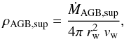 (5)where ṀAGB and Ṁsup are the mass loss rates of the AGB and the superphase AGB winds, respectively. Based on observational results (Neri et al. 1992; Pardo et al. 2004; Sánchez-Contreras et al. 2004; Nakashima et al. 2007; Bujarrabal et al. 2010; Lee et al. 2013), we chose ṀAGB = 10-5 M⊙ yr-1, Ṁsup = 10-4 M⊙ yr-1vw = 15 km s-1, rw = 3.6 × 1015 cm (equivalent to 6 pixels in the finest grid) and a constant temperature Tw = 100 K (this initial constant temperature acquires a decreasing profile with distance r, as the time-integration proceeds).
Parameters employed in the models.
The bipolar outflow was injected at the center of the computational domain inside a cylindrical volume with radius rj and length lj, both equal to rw. The jet axis precesses, describing a cone with a half-opening angle α. The precession period τp is related to the dynamical time τdyn and the orbital period τo by τdyn = p τp and τp = q τo, where p and q a pair of free dimensionless parameters (Velázquez et al. 2012; Velázquez et al. 2013). The jet velocity is given by 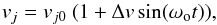 (6)where ωo is 2π/τo, vj0 is the mean velocity and Δv is the amplitude of velocity variation. The semiaperture angle α, the mean jet velocity vj0, and the initial number density nj were set to 15°, 400 km s-1 and 106 cm-3, respectively, for all models. The amplitude of the velocity variation was set to vj0/2 for all models. With these values for vj0 and nj, the average mass-injection rate of the jet is Ṁj = 5.6 × 10⁻⁵ M⊙ yr-1.
In ~120 yr (the total integration time of our simulations) the bipolar outflow injects a total mass of 1.3 × 10⁻² M⊙ into the surrounding medium.
With these values of injected mass and mean jet velocity, the linear momentum injected by the jet (in 120 yr) is 4.4 M⊙ km s-1, which agrees with the observational estimate of 4 M⊙ km s-1 (Bujarrabal et al. 2001). The value of q = τp/τo gives the m2/m1 ratio, employing the results of Terquem et al. (1999) and Raga et al. (2009) (see Table 3). We set m1 = 0.5 M⊙ (of the star which launches the jets) and the eccentricity e = 0.5 (actually, the value of e has little influence on the overall PN morphology, see Velázquez et al. 2013). In Table 3 we also list the values of the orbital period and radius employed in our models.
5.2. Numerical results
Velázquez et al. (2012, 2013) have shown that a precessing jet in a binary system with a time-dependent velocity produces nebulae with multipolar morphology. A quadrupolar morphology similar to CRL 618 is obtained by setting q = 2, 3 or 4. Because the adopted velocity variability period is the orbital period, and to have three or four ejections for each lobe along the 120 yr, we chose p = 4, for the case with q = 2 (model M1a), p = 3 for q = 3 (model M2a), and p = 2 for q = 4 (model M3a).
We also carried out three more runs (M1b, M2b, and M3b) for which the mean velocity vj0 (see Eq. (6)) was modified to be a decreasing function of time. For simplicity, we imposed a linear decrease with a rate of 3 km s-1 yr-1 (i.e. vj0, after t = 120 yr, decreases to 10% of its initial value).
As discussed in Sect. 5.3, such a systematic decrease in the ejection velocity is needed to reproduce the proper motions of CRL 618. This decrease in vj0 with time could be the result of the presence of a longer-period ejection velocity variability mode, but the currently observed lobes of CRL 618 do not give appropriate constraints for the amplitude and period of this mode.
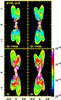 |
Fig. 8 Synthetic [S ii] emission maps obtained from models M1a (bottom panels) and M1b (top panels). The right panels display the yz projection for both models, while the left panels display the xz projection. The angle between the precession axis and the plane of sky was set to 25° for all models. The vertical color bar gives the [S ii] flux in units of erg s-1cm-2sr-1. The vertical and horizontal axes are given in units of 1017 cm. |
From the density and temperature distributions given by the numerical simulations, synthetic [S ii] emission maps were computed for all models. Figure 8 displays the maps obtained for models M1a (bottom panels) and M1b (top panels) for the xz- and yz-projections, at an integration time of 120 yr. The synthetic maps obtained for models M2a and M2b (models M3a and M3b) are shown in Fig. 9 (Fig. 10). These maps were obtained considering that the z-axis is tilted by 25°, with respect to the plane of the sky.
To explore whether or not our predicted maps show a small-scale structure similar to that observed in the lobes of CRL 618, we applied the wavelet analysis (as described in Sect. 3.1) to the synthetic map of the M2b simulation (yz-projection, at an integration time of 120 yr). The scale lengths of wavelets along the x- and y-axis were taken to have integer values from 1 to 60 pixels (i.e. from  to
to  ). The results are shown in Fig. 11.
On these synthetic maps, we also carried out the proper motion study that was performed for the observations (described in Sect. 3.2). To do this, the simulations were restarted from the output corresponding to an integration time of 120 yr and were left to evolve 10 yr longer. The results of the proper-motion study are shown in Figs. 12 and 13.
5.3. Comparison with observations
For all the computed models, emission structures similar to the jets of CRL 618 were obtained. As mentioned above, a quadrupolar morphology is predicted for all models presented in this work (the yz-projection maps of models M3a and M3b display a bipolar morphology). All synthetic maps show leading bow-shocks together with several arcs/rings and knots with a qualitative similarity to the morphology of the jets of CRL 618. However, our synthetic maps show an overall point-symmetric morphology, which is not observed in the CRL 618 images.
As mentioned above, the wavelet analysis was applied to the predicted [S ii] images (see Figs. 12 and 13). For this analysis, the synthetic map obtained from model M2b was rotated so that the jet axes lay parallel to the y-axis. The angular distance was measured from the jet injection point and the adopted distance to the object was 1 kpc. These figures show the ax,k and ay,k as a function of y for the two predicted jets, and the position of the local intensity maxima (i.e. (xk,y) for k = 1,2,3) are superimposed on the [S ii] synthetic image.
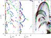 |
Fig. 11 Wavelet study performed on the top-left lobe or jet of the model M2b. The [S ii] image obtained from this model at a t = 120 yr integration time is shown in the right panel. For each y, the location of the three maxima of the intensity map are shown as dots superimposed on this image (first maximum in red, second maximum in green and third maximum in blue). The characteristic sizes (ax,k in the left panel; ay,k in the central panel) are shown as a function of position y along the jet axis. |
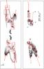 |
Fig. 12 Left panel: proper motions of the individual features in the synthetic [S ii] map (model M2b) together with the boxes in which the cross-correlations were made. The red arrows show the computed proper motions. The length of each arrow is proportional to the proper motion. Right panel: proper motions of the individual knots of CRL 618, included for comparison. Both images are shown to the same spatial scale. The vertical arrow at the top right shows a proper motion of 300 km s-1. |
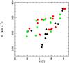 |
Fig. 13 Tangential velocity of the individual features in the synthetic [S ii] map obtained for model M1b (black), M2b (red) and M3b (green) at a t = 120 yr integration time as a function of distance to the jet injection point. |
When we applied the wavelet analysis to this synthetic image we obtained the typical sizes of the small-scale structure. The compact knots have widths across the jets ≤6 × 1015 cm (i.e.  ) and show a V-shaped structure in the ay,k vs. y plot. Some of the leading bow-shocks (as seen in Fig. 11) have small widths across the jet (which are more or less constant, with ax,k ≃ 6 × 1015 cm), and a V-shaped structure in the ay,k – y diagram. The elongation of these V-shaped structures decreases from
  at their edges to ~
 at the intensity peak. The wavelet analysis allows us to characterize the elongated structures with ay,k values ranging from
  to (i.e. 1.8 × 1016 cm to 3 × 1016 cm) which are similar to the elongated structures detected in the jets of CRL 618. The observed morphological classes (i.e., knots, bow-shocks, elongated structures and arcs) also appear in the wavelet analysis of the predicted [S ii] maps. Moreover, the sizes of the predicted emission features clearly agree with the observed ones.
We carried out the proper-motion study as described in Sect. 3.2, using two [S ii] emission maps computed for two epochs at a 10 yr time interval. The results obtained with the model M2b (projection yz) are shown in Figs. 12 and 13. Figure 12 shows the boxes used for the calculation, and the resulting proper motions are shown as red arrows. We clearly see that all features show proper motions in the direction of the corresponding jet axis, a result found in all six models.
From the predictions of models a, we find tangential velocities from 200 to 500 km s-1, which are higher than the observed values (see Sect. 4.2). The tangential velocities derived from the M1a and M2a models show a quite wide dispersion, and basically no correlation is seen between the tangencial velocity and the distance to the central source. To reproduce the apparent acceleration of the knots of the jet of CRL 618 with distance, it was necessary to superimpose on the periodic velocity variability a trend of decreasing ejection velocity (vj0) over time. We computed three models (M1b, M2b and M3b) for which the mean jet velocity is a linear decreasing function of time. For these two models we found tangential velocities ~100 to 350 km s-1. The results obtained for model M2b are presented in Fig. 13. As a function of distance d, vt shows a quite wide scatter, and a general trend of increasing velocities from the inner knots to the leading bow-shocks. The vt vs. d plot shows a more or less monotonic growth, reaching a value of ~350 km s-1 at the outer bow-shocks. Similar results were found for model M1b. All three models (M1b, M2b, and M3b) reproduce the distance dependence of the tangential velocities observed in CRL 618.
An obvious difference between CRL 618 and all of our models is the fact that while the models show point-symmetries between the correponding components of the outflow lobes, CRL 618 does not show such symmetries. The point symmetrical structure in our models is a direct result of the fact that we imposed a point-symmetrical, precessing jet/counterjet ejection.
This symmetry discrepancy between our models and CRL 618 indicates that the structures observed in this object do not correspond to point-symmetrical ejections. The lack of point-symmetry could be an indication of the presence of effects similar to those found in the models of Montgomery (2012), in which the tidally induced disk precession changes the point of impact of an accretion column from a mass-exchanging binary companion. This process results in clear differences between the two faces of the accretion disk and would probably result in substantial differences between the two outflow lobes produced by the inner disk regions.
6. Summary and discussion
We have reanalyzed the [S ii] HST images of CRL 618 obtained by Trammell & Goodrich (2002) and Balick et al. (2013). We applied an anisotropic wavelet analysis technique to calculate the characteristic sizes along and across the CRL 618 jets. From this analysis, we found four morphological classes: compact knots (which have sizes along and across the axis ~6 × 1015 cm), outermost bow-shocks (with widths ranging from ~1.5 × 1015 cm to ~1016 cm, and sizes smaller than ~1.2 × 1016 cm along the jet), elongated features (with ax,k ≤ ~ 6 × 1015 cm, ay,k ≥ 3 × 1016 cm), and arcs.
From the archival [S ii] HST images of CRL 618 with a 10.7 yr time base, we carried out proper-motion measurements of the knots, arcs, and bow-shocks observed in the lobes of CRL 618, computing the two-dimensional cross-correlation function of the emission detected within the chosen boxes. The proper motions were calculated through a parabolic fit to the peak of the cross-correlation. We found proper motions which are well-aligned with the jets axes (either the J1, J2, J1′ or J2′ axis), and tangential velocities ranging from 60 to 430 km s-1. These velocities agree to within 15% with the Hα proper motions of Balick et al. (2013) after correcting these velocities for the diastance of 0.9 kpc adopted by these authors. Fom our proper-motion measurements and the distance to the central source, we calculated the kinematic age for several features. We found τkin ~ 50 to 100 yr, ages increasing with the distance to the central source.
We found that the tangential velocity is a monotonically increasing function of distance d, with the highest proper motions at the outermost bow-shocks (with velocities up to 430 km s-1). A ramp of increasing radial velocities versus distance is seen in the outer regions of the bright lobe of CRL 618 (Sánchez Contreras et al. 2002; Riera et al. 2009). Therefore, the jet ejection velocity shows a monotonic increase with distance to the central source, which we interpret as a systematic decrease of the ejection velocity over time.
We modeled the jets of CRL 618 as a precessing jet with a time-dependent ejection velocity that is launched from the secondary star of a binary system. The [S ii] intensity maps predicted for the sinusoidal ejection velocity models have morphologies that agree with the [S ii] HST images of CRL 618. The increase of the tangential velocity (and also the increase of radial velocity) with distance to the central source requires a mean jet velocity that varies over time. The dependence of the tangential velocities with distance to the central source can be reproduced when we impose a linear decrease of the mean vj0 over time.
From the comparisons we made between the structure and proper motions observed in CRL 618 and predictions from 3D jet simulations, we predict the presence of the following elements:
-
a well-collimated, bipolar ejection,
-
a precession of the outflow axis,
-
an approximately periodic time-variability of the outflow velocity with a period on the order of 15 yr (the orbital one),
-
a general, long-term trend of decreasing outflow velocities from dynamical timescales of ~50 yr toward more recent times.
It is currently not possible to say whether or not the long-term trend of decreasing outflow velocity vs. time might be part of a longer-period, quasi-periodic variability. If that were the case, new knots along the CRL 618 jets at future times would show larger proper motions. The younger present-day astronomers might yet be able to observe this effect.
Acknowledgments
A.Ri., R.E., and A.C. are partially supported by Spanish MCI grants AYA2008-06189-C03 and AYA2011-30228-C03, and FEDER funds. PFV and ACR acknowledge support from CONACyT grants 61547,101356, 101975, 167611, and UNAM DGAPA grant IN105312.
References
- Balick, B., Huarte-Espinosa, M., Frank, A., et al. 2013, ApJ, 772, 20 [NASA ADS] [CrossRef] [Google Scholar]
- Bujarrabal, V., Castro-Carrizo, A., Alcolea, J., & Sánchez Contreras 2001, A&A, 377, 868 [NASA ADS] [CrossRef] [EDP Sciences] [Google Scholar]
- Bujarrabal, V., Alcolea, J., Soria-Ruiz, R., et al. 2010, A&A, 521, A3 [Google Scholar]
- Carsenty, U., & Solf, J. 1982, A&A, 106, 307 [NASA ADS] [Google Scholar]
- Cernicharo, J., Guelin, M., Penalver, J., Martin-Pintado, J., & Mauersberger, R. 1989, A&A, 222, L1 [NASA ADS] [Google Scholar]
- Cox, P., Huggins, P. J., Maillart, J.-P., et al. 2003, ApJ, 586, L87 [NASA ADS] [CrossRef] [Google Scholar]
- Dennis, T. J., Cunningham, A. J., Frank, A., et al. 2008, ApJ, 679, 1327 [NASA ADS] [CrossRef] [Google Scholar]
- Goodrich, R. W. 1991, ApJ, 376, 654 [NASA ADS] [CrossRef] [Google Scholar]
- Grosdidier, Y., Moffat, A. F. J., Blais-Ouellette, S., Joncas, G., & Acker, A. 2001, ApJ, 562, 753 [NASA ADS] [CrossRef] [Google Scholar]
- Guerrero, M. A., Miranda, L. F., Riera, A., et al. 2008, ApJ, 683, 272 [NASA ADS] [CrossRef] [Google Scholar]
- Haro-Corzo, S. A. R., Velázquez, P. F., Raga, A. C., Riera, A., & Kajdic, P. 2009, ApJ, 703, L18 [NASA ADS] [CrossRef] [Google Scholar]
- Kwok, S., & Bignell, R. C. 1981, ApJ, 276, 544 [Google Scholar]
- Kwok, S., & feldman, P. A. 1984, ApJ, 247, 67 [Google Scholar]
- Lee, C.-F., & Sahai, R. 2003, ApJ, 586, 319 [NASA ADS] [CrossRef] [Google Scholar]
- Lee, C.-F., Hsu, M.-C., & Sahai, R. 2009, ApJ, 696, 1630 [NASA ADS] [CrossRef] [Google Scholar]
- López, R., Riera, A., Raga, A. C., et al. 1996, MNRAS, 282, 470 [NASA ADS] [CrossRef] [Google Scholar]
- Martín-Pintado, J., Bujarrabal, V., Bachiller, R., Gómez-González, J., & Planesas, P. 1988, A&A, 204, 242 [NASA ADS] [Google Scholar]
- Mendoza, C. 1983, Proc. IAU Symp. 103, Planetary Nebulae, ed. D. Flower (Reidel: Dordrecht), 143 [Google Scholar]
- Miranda, L. F., Blanco, M., Guerrero, M. A., & Riera, A. 2012, MNRAS, 421, 1661 [NASA ADS] [CrossRef] [Google Scholar]
- Montgomery, M. M. 2012, ApJ, 753, L27 [NASA ADS] [CrossRef] [Google Scholar]
- Morris, M. 1987, PASP, 99, 1115 [NASA ADS] [CrossRef] [Google Scholar]
- Nakashima, J.-I., Fong, D., Hasegawa, T., et al. 2007, AJ, 134, 2035 [NASA ADS] [CrossRef] [Google Scholar]
- Neri, R., García-Burillo, S., Guelin, M., et al. 1992, A&A, 262, 544 [NASA ADS] [Google Scholar]
- Pardo, J. R., Cernicharo, J., Goicoechea, J. R., & Phillips, T. G. 2004, ApJ, 615, 495 [NASA ADS] [CrossRef] [Google Scholar]
- Raga, A. C., Navarro-González, R., & Villagrán-Muniz, M. 2000, Rev. Mex. Astron. Astrofis., 36, 67 [NASA ADS] [Google Scholar]
- Raga, A. C., de Gouveia Dal Pino, E. M., Noriega-Crespo, A., Mininni, P. D., & Velázquez, P. F. 2002, A&A, 392, 267 [NASA ADS] [CrossRef] [EDP Sciences] [Google Scholar]
- Raga, A. C., Esquivel, A., Velázquez, P. F., et al. 2009, ApJ, 707, L6 [NASA ADS] [CrossRef] [Google Scholar]
- Reipurth, B., Raga, A. C., & Heathcote, S. 1992, ApJ, 392, 145 [NASA ADS] [CrossRef] [Google Scholar]
- Riera, A., Raga, A. C., Reipurth, B., et al. 2003, AJ, 126, 327 [NASA ADS] [CrossRef] [Google Scholar]
- Riera, A., Binette, L., & Raga, A. C. 2006, A&A, 455, 203 [NASA ADS] [CrossRef] [EDP Sciences] [Google Scholar]
- Riera, A., Raga, A. C., Velázquez, P. F., et al. 2009, Protostellar Jets in Context, eds. K. Tsinganos et al. (Berlin: Springer-Verlag), Ap&SS Proc. Ser., 603 [Google Scholar]
- Riera, A., Raga, A. C., Velázquez, P. F., et al. 2011, A&A, 533, A118 [NASA ADS] [CrossRef] [EDP Sciences] [Google Scholar]
- Sánchez Contreras, C., & Sahai, R. 2004, ApJ, 602, 960 [NASA ADS] [CrossRef] [Google Scholar]
- Sánchez Contreras, C., Sahai, R., & Gil de Paz, A. 2002, ApJ, 578, 269 [NASA ADS] [CrossRef] [Google Scholar]
- Sánchez Contreras, C., Bujarrabal, V., Castro-Carrizo, A., Alcolea, J., & Sargent, A. 2004, ApJ, 617, 1142 [NASA ADS] [CrossRef] [Google Scholar]
- Soker, N., & Rappaport, S. 2000, ApJ, 538, 241 [NASA ADS] [CrossRef] [Google Scholar]
- Soria-Ruiz, R., Bujarrabal, V., & Alcolea, J. 2013, A&A, 559, A45 [NASA ADS] [CrossRef] [EDP Sciences] [Google Scholar]
- Tafoya, D., Loinard, L., Fonfría, J. P., et al. 2013, A&A, 556, A35 [NASA ADS] [CrossRef] [EDP Sciences] [Google Scholar]
- Terquem, C., Eislöffel, J., Papaloizou, J. C. B., & Nelson, R. P. 1999, ApJ, 512, L131 [NASA ADS] [CrossRef] [EDP Sciences] [Google Scholar]
- Trammell, S. R., & Goodrich, R. W. 2002, ApJ, 579, 688 [NASA ADS] [CrossRef] [Google Scholar]
- Trammell, S. R., Dinerstein, H. L., & Goodrich, R. W. 1993, ApJ, 402, 249 [NASA ADS] [CrossRef] [Google Scholar]
- van Leer, B. 1982, in Proc. Numerical Methods in Fluid Dynamics, ed. E. Krause (Berlin: Springer), Lect. Notes Phys., 507 [Google Scholar]
- Velázquez, P. F., Riera, A., & Raga, A. C. 2004, A&A, 419, 991 [NASA ADS] [CrossRef] [EDP Sciences] [Google Scholar]
- Velázquez, P. F., Gómez, Y., Esquivel, A., & Raga, A. C. 2007, MNRAS, 382, 1965 [NASA ADS] [Google Scholar]
- Velázquez, P. F., Steffen, W., Raga, A. C., et al. 2011, ApJ, 734, 57 [NASA ADS] [CrossRef] [Google Scholar]
- Velázquez, P. F., Raga, A. C., Riera, A., et al. 2012, MNRAS, 419, 3529 [NASA ADS] [CrossRef] [Google Scholar]
- Velázquez, P. F., Raga, A. C., Cantó, J., Schneiter, E. M., & Riera, A. 2013, MNRAS, 428, 1587 [NASA ADS] [CrossRef] [Google Scholar]
- Westerbrook, W. E., Willner, S. P., Merrill, K. M., et al. 1975, ApJ, 202, 407 [NASA ADS] [CrossRef] [Google Scholar]
All Tables
All Figures
|
Fig. 1 CRL 618 in the 1998.89 (left) and 2009.60 (right) [S ii] images shown to the same scale and pixel size (0 |
| In the text | |
|
Fig. 2 Bright (east) lobe in the 1998.89 (left) and 2009.60 (right) [S ii] images. Several features along regions J1 and J2 are marked and labeled. Changes in the structure of the labeled features between both epochs are discussed in the text. The red arrows show the assumed identifications of corresponding knot pairs in the two epochs. |
| In the text | |
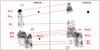 |
Fig. 3 Same as Fig. 2, but for the jets of the faint (west) lobe (labeled J1′ and J2′). |
| In the text | |
|
Fig. 4 First-epoch [S ii] image of the J1 (bottom) and J2 (top) jets and the characteristic sizes of the small-scale features observed in the optical lobes (ax,k (left) and ay,k (right)) as a function of position y along the jet axis, obtained from the wavelet analysis. The k = 1 peaks are represented in red, k = 2 in green, and k = 3 in blue. Three examples of the compact knots (K), arc, and leading bow-shock (BS) classes are labeled. |
| In the text | |
|
Fig. 5 Same as Fig. 4, but for the faint lobe. The J1′ jet is presented in the bottom panel. The J2′ jet is shown in the top panel. Three examples of the compact knots (K), elongated structures (ES), and leading bow-shock (BS) classes are labeled. |
| In the text | |
|
Fig. 6 Proper motions of the individual features in the jets of CRL 618. First-epoch [S ii] image of CRL 618 together with the boxes in which the cross-correlations were made (see text). The red boxes correspond to individual knots. Features that include more than one knot (as E1, E9 and W3) are marked in green. The blue boxes were used to measure the proper motion of the J1, J2, J1′ and J2′ jets. The arrows show the computed proper motions. The length of each arrow is proportional to the proper motion. The vertical arrow at the top right shows a proper motion of 300 km s-1. |
| In the text | |
|
Fig. 7 Tangential velocity as a function of distance to the central H II region. Top panel: faint lobe (J1′ (circles), J2′ (squares)). Bottom panel: bright lobe (J1 (circles), J2 (squares)). |
| In the text | |
|
Fig. 8 Synthetic [S ii] emission maps obtained from models M1a (bottom panels) and M1b (top panels). The right panels display the yz projection for both models, while the left panels display the xz projection. The angle between the precession axis and the plane of sky was set to 25° for all models. The vertical color bar gives the [S ii] flux in units of erg s-1cm-2sr-1. The vertical and horizontal axes are given in units of 1017 cm. |
| In the text | |
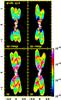 |
Fig. 9 As Fig. 8, but for models M2a (bottom panels) and M2b (top panels). |
| In the text | |
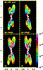 |
Fig. 10 As Fig. 8, but for models M3a (bottom panels) and M3b (top panels). |
| In the text | |
|
Fig. 11 Wavelet study performed on the top-left lobe or jet of the model M2b. The [S ii] image obtained from this model at a t = 120 yr integration time is shown in the right panel. For each y, the location of the three maxima of the intensity map are shown as dots superimposed on this image (first maximum in red, second maximum in green and third maximum in blue). The characteristic sizes (ax,k in the left panel; ay,k in the central panel) are shown as a function of position y along the jet axis. |
| In the text | |
|
Fig. 12 Left panel: proper motions of the individual features in the synthetic [S ii] map (model M2b) together with the boxes in which the cross-correlations were made. The red arrows show the computed proper motions. The length of each arrow is proportional to the proper motion. Right panel: proper motions of the individual knots of CRL 618, included for comparison. Both images are shown to the same spatial scale. The vertical arrow at the top right shows a proper motion of 300 km s-1. |
| In the text | |
|
Fig. 13 Tangential velocity of the individual features in the synthetic [S ii] map obtained for model M1b (black), M2b (red) and M3b (green) at a t = 120 yr integration time as a function of distance to the jet injection point. |
| In the text | |
Current usage metrics show cumulative count of Article Views (full-text article views including HTML views, PDF and ePub downloads, according to the available data) and Abstracts Views on Vision4Press platform.
Data correspond to usage on the plateform after 2015. The current usage metrics is available 48-96 hours after online publication and is updated daily on week days.
Initial download of the metrics may take a while.