| Issue |
A&A
Volume 559, November 2013
|
|
|---|---|---|
| Article Number | A83 | |
| Number of page(s) | 20 | |
| Section | Planets and planetary systems | |
| DOI | https://doi.org/10.1051/0004-6361/201220770 | |
| Published online | 20 November 2013 | |
Planets around stars in young nearby associations
Radial velocity searches: a feasibility study and first results⋆,⋆⋆,⋆⋆⋆
1
Institut de Planétologie et d’Astrophysique de Grenoble, UMR5274 CNRS,
Université Joseph Fourier,
BP 53,
38041
Grenoble Cedex 9,
France
e-mail: anne-marie.lagrange@obs.ujf-grenoble.fr
2
European Southern Observatory, Casilla 19001,
19 Santiago,
Chile
3
European Southern Observatory, Karl-Schwarzschild-Str. 2, 85748
Garching bei Munchen,
Germany
4
Observatoire de Genève, Université de Genève,
51 ch. des Maillettes,
1290
Versoix,
Switzerland
Received: 21 November 2012
Accepted: 20 May 2013
Context. Stars in young nearby associations are the only targets that allow giant planet searches in the near future, at all separations by coupling indirect techniques, such as radial velocity (RV) and deep imaging. These stars are first priority targets for the forthcoming planet imagers on eight- to ten-metre class telescopes. Young stars rotate more rapidly and are more active than their older counterparts. Both effects can limit the ability to detect planets using RV.
Aims. We wish to explore the planet detection abilities of a representative sample of stars in close and young associations with RV data and to explore the complementarity between this technique and direct imaging.
Methods. We observed 26 such targets with spectral types from A to K and ages from 8 to 300 Myr with HARPS. We computed the detection limits with two methods, in particular, a method we have recently developed that takes the frequency distribution of the RV variations into account. We also attempted to improve the detection limits in a few cases by correcting for the stellar activity.
Results. Our A-type stars RV show high-frequency variations due to pulsations, while our F-K stars clearly show activity with more or less complex patterns. For F-K stars, the RV jitter and vsini rapidly decrease with star age. The data allow us to search for planets with periods typically ranging from 1 day to 100 days, and up to more than 500 days in a few cases. Within the present detection limits, no planet was found in our sample. For the bulk of our F-K stars, the detection limits fall to sub-Jupiter masses. We show that these limits can be significantly improved by correcting even partially for stellar activity, down to a few Neptune masses for the least active stars. The detection limits on A-type stars can be significantly improved, down to a few Jupiter-mass planets, provided an appropriate observing strategy. We finally show the tremendous potential of coupling RV and adaptive-optics deep imaging results.
Conclusions. The RV technique allows the detection of planets lighter than Jupiter, reaching a few Neptune masses around young stars aged typically 30 Myr or more. Detection limits increase at younger ages, but (sub-)Jupiter mass planets are still detectable. In the next few years, using complementary techniques will allow a full exploration of the Jupiter-mass planets’ content of many of these stars.
Key words: techniques: radial velocities / techniques: high angular resolution / planets and satellites: detection
Based on observations made with the ESO3.6m/Harps spectrograph at La Silla.083.C-0794(ABCD); 084.C-1039(A); 084.C-1024(A).
Appendices A and B are available in electronic form at http://www.aanda.org
Tables of radial velocities are only available at the CDS via anonymous ftp to cdsarc.u-strasbg.fr (130.79.128.5) or via http://cdsarc.u-strasbg.fr/viz-bin/qcat?J/A+A/559/A83
© ESO, 2013
1. Introduction
Thanks to hundreds of discoveries for more than 15 years1, mainly coming from radial velocity (RV) and transit surveys, our knowledge of exoplanets has dramatically improved. We know that exoplanets are frequent around solar-type, main sequence (MS) stars: more than 50% have planets (all masses, Mayor et al. 2011) and about 15% have planets with masses higher than 50 MEarth. An unexpected diversity of planet properties, such as separations, eccentricities, and orbital motions (for example retrograde orbits discovered thanks to the Rossiter-McLaughlin effect), was revealed for short -or intermediate – period planets. This suggests that the dynamics due, for example, to planet-planet interactions or early disk-planet interactions plays an important role in building planetary systems.
Giant planets play an important role because they carry most of the planetary systems’ mass. They therefore strongly impact the dynamics and fate of lighter planets, and, consequently, the final architecture of the planetary systems. Giant planets also affect the detectability of lighter planets as far as indirect methods are concerned. Even though giant planets represent the majority of the planets detected so far, we are far from having a clear picture of their occurrence, variety, and properties. RV and transit explorations are indeed still limited to planets orbiting within 5 AU of their parent stars, while current deep (adaptive-optics, hereafter AO) imaging, which is meant to detect more distant planets, is not sensitive enough for MS stars, except around a few young early-type stars that have already reached the MS Stars in young nearby associations (see for example Torres et al. 2008; Zuckerman & Song 2004) are therefore the best targets for a complete giant planet exploration, if combining the data obtained with forthcoming planet imagers, such as SPHERE at the VLT (Beuzit et al. 2008) or GPI at Gemini (Macintosh et al. 2008), and high-precision spectrographs. In addition, these data could be combined in the future with astrometric measurements when available.
Compared to mature MS stars, limited effort has been devoted so far to the search for planets around young stars with RV techniques. To our knowledge, the only significant surveys have been performed by Paulson et al. (2004) on 94 stars members of the Hyades (aged about 600 Myr) and on 61 stars members of various moving groups (MGs) or stellar associations aged between 12 and 300 Myr (Paulson & Yelda 2006). In both cases, high spectral resolution data in the range 40 000–70 000 were used. The internal errors were 3–5 m/s and ≃10 m/s. The Hyades stars were found to be weakly active, with stellar jitters in the range 10–20 m/s (average value = 16 m/s). No planet was detected with masses down to 1–2 MJup, down to the sub-Jupiter mass regime in a few cases, and with periods typically of 1–2 years or less. In the second case, no planet was detected with a detection limit reaching 1–2 MJup, for periods up to six days for the oldest stars, while the detection limits fell into the brown dwarf regime for the youngest targets (members of the β Pic group).
Stellar activity can mimic planet signatures (Desort et al. 2007), and great care must be taken when analysing RV data. In the past, two detections were announced around TW Hya (Setiawan et al. 2007), and BD +20 1790 (Hernán-Obispo et al. 2010), but were strongly debated (Figueira et al. 2010). Bailey et al. (2012) used NIRSPEC at Keck to observe a set of 20 young stars with high-precision spectroscopy in the near-IR, where line shifts due to spot-induced activity are expected to be smaller than at optical wavelengths. Detection limits of 8 MJup (respectively 17 MJup) were obtained for periods of three days (respectively 30 days) periods. Crockett et al. (2012) used CSHELL for similar purposes on nine T Tauri stars and showed that for these stars, the jitter in the near IR was reduced by a factor 2–3 compared to the jitter measured in the optical range. No planet was firmly detected. Finally, we unambiguously detected a 2.8 MJup giant planet orbiting with a 320-day period, a 150 Myr, weakly active star (Borgniet et al. 2013).
We investigate here the potential of high-precision optical spectroscopy in searching for giant planets around 26 stars, which are members of close-by young associations, since these stars are potential targets of the SPHERE NIRSUR survey aimed at imaging giant planets. Section 2 describes our targets and observing log. Section 3 presents the data analysis. The results are shown and discussed in Sect. 4. In Sect. 5, we show how such results can be coupled to deep imaging detection limits to perform a complete exploration of giant planets in the environements of these young and close stars.
2. Targets and observations
The bulk of our sample is made of 22 bright (V ≤ 9), nearby (d ≤ 80 pc), young (≤200 Myr) stars identified in young MGs and from systematic spectroscopic surveys. Four other stars with ages greater than 200 Myr were observed: HD 90905, HD 109536, HD 105690, and HD 188828. The 26 stars are listed in Table 1. Our sample includes eight A-type stars, four F-type stars, ten G-type stars and four K-type stars. Several of them are known to have debris disks (Rodriguez & Zuckerman 2012). In several cases, peculiar disks properties (shapes, offsets) suggest that inner planets could be present.
Target list and stellar parameters.
We provide some details here about a few peculiar targets. Unless otherwise indicated, relative disk luminosities Ldisk/Lstar are from Moór et al. (2006) or Rhee et al. (2007), and binary indications from Rodriguez & Zuckerman (2012):
-
HD 39060(β Pictoris ) is surrounded by aseen edge-on disk (Ldisk/Lstar=2 × 10-3), as well as a planet detected in direct imaging (Lagrange et al. 2009b, 2010). Detection limits in deep imaging fall in the giant planet regime. A study of RV data allowed Lagrange et al. (2012) to set an upper limit to the dynamical mass of β Pictoris b.
-
HD 61005 (The Moth) is surrounded by a thin and narrow disk that is resolved in near-IR (Hines et al. 2007; Buenzli et al. 2010, and references therein). The disk is seen as a ring inclined by 84 degrees with respect to pole-on and is offset from the star center. In addition, streamers are observed at the edge of the ring. Detection limits in deep imaging fall in the giant planet regime.
-
HD 172555 belongs to the β Pictoris MG (Zuckerman et al. 2001). It has a spectral type similar to that of β Pictoris but an IR excess smaller than that of β Pictoris (Ldisk/Lstar = 8 × 10⁻⁴). It is also part of a wide binary system.
-
HD 174429 (PZ Tel) has an IR excess (Ldisk/Lstar = 9 × 10⁻⁵). A brown dwarf companion with a 20–40 MJup mass is present with a projected separation of 0.3′′ representing 15 AU (Biller et al. 2010). Given the companion Δ J (5.6 mag), its expected V − J (5.5–6.5 mag), its mass and age, and the V − K (1.2 mag) of the star itself, the contrast at optical wavelengths between PZ Tel and its companion is about 9–10 mag. The companion’s contribution to the visible flux within the Harps fibre (1′′) is therefore negligeable.
-
HD 181327 is a member of the β Pictoris MG, with a large IR excess (Ldisk/Lstar = 2 × 10⁻³Lebreton et al. 2012). A debris disk has been resolved in near IR by Schneider et al. (2006). It shapes a ring located at 90 AU and inclined by about 30 degrees from face-on.
-
HD 216956 (Fomalhaut) is also surrounded by a debris disk (Ldisk/Lstar = 8 × 10⁻⁵) seen as a narrow ring at 115 AU (Kalas et al. 2005), inclined by 24 degrees from edge-on and offset from the star. It may also be surrounded by a planet orbiting just inside the ring (Kalas et al. 2008), and shaping its sharp inner edge (Chiang et al. 2009), but this planet is still being debated (Janson et al. 2012). Recently Lebreton et al. (2013) showed that warm dust is also present within AUs from the star.
-
HD 218396 (HR8799) is surrounded by a system of four planets detected in imaging with projected separations between 15 and 70 AU (Marois et al. 2008, 2010). A thin debris disk (Ldisk/Lstar = 2 × 10⁻⁴) has also been resolved at sub-mm wavelengths (Patience et al. 2011) and has an inclination of 20–50 degrees from face-on (Kalas et al. 2010).
We have obtained more than 2000 high resolution (R ≃ 115 000) and high signal-to-noise (S/N) spectra of our targets with the fibre-fed spectrograph Harps (Mayor et al. 2003) at the La Silla 3.6 m telescope. In the case of β Pictoris, we used, in addition to our data, a few data available in the archive and obtained with the same set-up. The spectra cover a wavelength range between 3800 and 6900 Å. During our runs, we usually recorded two consecutive spectra for each telescope pointing. In the following, one pointing is referred to as one epoch. Since our main goal was to look for short-period planets (100 days or less), we recorded several spectra of each target during each run whenever possible. In addition, we also recorded whenever possible spectra at two or three different epochs during one night, to identify possible high-frequency RV variations. For the brightest stars, we did not consider spectra with saturation that could affect the RV measurements. We report in Table 2 information about each star observation. The timespan varies between a few hours for three of our targets and 1912 days. The stars with a long timespan are early-type stars that happened to be part of a previous survey of A-F stars described in Lagrange et al. (2009a). The exposure times were computed to get a S/N larger than 200 at 550 nm in most cases. This corresponds to exposure times between less than one minute for the brightest targets and 15 for the faintest ones.
Observation results and typical detection limits.
Finally, for some of the earliest types, generally pulsating stars, we performed continuous observations over typically one to two hours to check that short-term pulsations are indeed present and to estimate their amplitude.
3. Data analysis
3.1. RV measurements
The RV were computed using SAFIR, a tool dedicated to measuring accurate RVs on fast rotators, as described in Galland et al. (2005), and based on the Fourier interspectrum method developed by Chelli (2000). SAFIR has been extensively used, in particular in RV surveys of rapidly rotating stars (Lagrange et al. 2009a). SAFIR input data are the extracted 2D spectra provided by the Data Reduction Software (DRS) pipeline and the related wavelength calibration coefficients. SAFIR takes care of the blaze correction, as well as bad-pixel correction (Galland et al. 2005). The errors associated to the individual RV measurements typically range between 1.5 m/s for the slowly rotating stars to 30–40 m/s for the fast-rotating stars. The values obtained for slowly rotating stars are similar to those obtained by the HARPS DRS; they show that the instrument internal errors are very low. Lomb-Scargle periodograms of the RV variations were also computed for each target.
3.2. Line profile variations and activity indicators
For stars with vsini below typically 100 km s-1 and spectral types later than A3V, it is possible to compute the bisector velocity spans (BVS) using the cross-correlation function, as shown in Lagrange et al. (2009a). Typical examples are provided in Fig. 1 for an active star (upper panels) and a pulsating one (lower panels). The relation between BVS and RV is useful for further characterizing the temporal RV variations whenever present. A correlation between the RV and BVS variations indicates that the RV are due to stellar activity (Desort et al. 2007), while pulsation-dominated variations instead induce uncorrelated (RV, BVS) variations. We also computed the vsini using the cross-correlation function for the low to moderately rotating stars, and the obtained values are given in Table 2.
For active stars, we also computed the S-index that measures the amount of chromospheric activity, and derived the Ca index  according to Duncan et al. (1991)2. In the case of the Sun, there is a correlation between the long-term Ca emission variability and the RV variability (see Meunier & Lagrange 2013, and references therein). For solar-type MS stars, a correlation between the long-term photometric variability and the Ca emission is also observed (see in particular Lockwood et al. 2007): the brightness increases when the Ca emission increases. This is consistent with the fact that the long-term photometric variations are, as for the Sun, dominated by plages. Correlations between RV and Ca emission have been searched for (Santos et al. 2010; Isaacson & Fischer 2010; Boisse et al. 2009; Dumusque et al. 2011), but only rarely reported (Dumusque et al. 2011, and references therein). However, instrumental artefacts such as diffused light could alter the Ca emission measurements and/or the RV measurements (the long term stability must be ensured to a few m/s) and may therefore prevent finding such a correlation. For young solar-type stars, the situation is even less clear, as much less data are available. The long-term photometric variations are anti-correlated with chromospheric activity variations; i.e., the brightness decreases when the Ca emission increases, in contrast to older Sun-like stars (Lockwood et al. 2007). This is interpreted as the photometric variations being spot-dominated.
For stars with a high enough vsini (i.e. larger than 15–20 km s-1) or with very strong emissions, the 1 Å wavelength range used to measure the Ca emission index is too narrow compared to the emission itself. Even though sophisticated modelling has been proposed to estimate the Ca index in such cases (Schröder et al. 2009), we did not make any attempt to do so, since the main purpose of the present paper is not to study stellar activity. In such cases no value is given in Table 2.
 |
Fig. 1 Upper panels: RV versus time, bisectors, BVS versus time and BVS versus RV for the active G-type star HD 183414. In the last panel, we indicate the slope of the (RV, BVS) correlation. Lower panels: same for the pulsating A-type star HD 216956. |
3.3. Detection-limit measurements
As extensively discussed in a previous dedicated paper (Meunier et al. 2012, hereafter MLB12), there are different ways to estimate detection limits associated to RV time series. We use two methods in the present paper, namely the “rms-based method” and the LPA method. Noticeably, we do not use the bootstrap method that, we showed, provides detection limits that are not as good as the LPA method and, in the case of pulsating stars, may provide unrealistic results. We refer to MBL12 for a detailed description of these methods and their respective merits. We briefly summarize the principles of the rms-based and LPA methods, and examples of the obtained detection limits are provided in Fig. 2.
The fastest method, the rms-based method, is based on the measured standard deviation (hereatfer rms) of the RV series and was first described in Lagrange et al. (2009a). In the rms-based method, we compute the RV produced by a planet with a given mass and period for the actual temporal sampling and then the rms of these simulated RV. This is done for 1000 orbital phases. The distribution of this rms is Gaussian. If the rms of the observed RV is lower than the average rms of the 1000 simulated RV, the planet is detectable. The level of confidence (detection probability) is obtained by comparing the standard deviation of the simulated distribution and the difference between the observed rms and the average value of the simulated distribution. We showed in Lagrange et al. (2009a) that, provided a very good temporal sampling is available, the rms-based detection limit in mass for a given period is similar to the mass of a planet that would produce an RV amplitude equal to 3 × rms(RV). In the following, the latter limit will be referred to as the “rms-based achievable limit”.
The LPA (local power analysis) method provides more accurate and lower detection limits when enough data are available (see below). Briefly, for a given period P, we compute the maximum of the periodogram of the observed RV in the range 0.75P–1.25P 3, and this provides a threshold for that period. Then, for a given planet (mass, period), we compare the maximum amplitude of the power spectrum of the RV induced by this planet on the same temporal sampling with that threshold, for 100 trials of the phase of the planet. If for all these trials, all “planet amplitudes” are above the threshold, then the planet mass is above the detection limit. We iterate on the planet mass until we reach a mass for which this condition is no longer met, indicating a mass below the detection limit. The smallest step we use is in general 0.1 MJup, but we choose a smaller step in a few cases to avoid a discretization of the detection limits. With our present set of data, we can use the LPA method for ten stars, for which more than 40 data points were available.
As expected, the LPA detection limits are much lower than the rms-based limits. To quantify the improvement, we computed the ratio between the rms-based and the LPA detection limits for each of the 200 periods considered, and then the median of the 200 ratio. The median ratio is typically a factor of 2 to 3, but may sometimes reach higher values (see Sect. 4). The improvement is due to the fact that the LPA method takes into account the variability of the power amplitude frequency, either due to an actual signal or to the temporal sampling, while the rms-based does not. The advantage of the rms-based is that the computation is fast and less sensitive to the number of data available. It provides an order of scale but a pessimistic estimation of the achievable detection limits (Lagrange et al. 2009a).
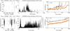 |
Fig. 2 Upper panels: RV versus time, periodogram of RV and detection limits (from left to right) for the G2V star HD 183414, covering a time span of 189 days. The detection limits have been computed using the rms-based method (black line), LPA (orange stars). Lower panels: same for the A5V star HD 39060 covering a time span of 2600 days. |
3.4. Search for circumstellar Ca in rapid rotators
Finally, as a by-product of these observations, we also used the spectra to search for narrow CaII absorption lines at the bottom of the rotationally broadened stellar lines. Such absorptions could indicate the presence of circumstellar gas, as present in the case of HD 39060 (e.g. Lagrange et al. 2000).
4. Results
4.1. RV time series and variability properties
We show in Appendix A the obtained RV times series for our 26 targets. The RV rms and amplitudes, as well as the BVS rms and amplitudes for stars with enough data points, are reported in Table 2. The average jitter of our eight A type stars is 237 m/s, while that of the three F-type stars is 35 m/s and that of the thirteen G-K stars is 131 m/s. The median is 67 m/s in the last case. For the stars for which the BVS could be computed, the average BVS is 61 m/s for the F-type stars and 74 m/s for the G-K type stars. We recall though that within a given spectral type range, there is a large dispersion of jitters due to the star ages (see below). Among the 14 F-K stars with at least two epochs4, only one, HD 224228, shows no detetectable level of RV variations, with an RV jitter below 5 m/s. Twelve stars have jitters larger than 5 m/s. Among them, only three have jitters larger than 150 m/s (referred to as “high amplitude variable stars”), five have jitters between 50 and 105 m/s (referred to as “medium amplitude variable stars”), and four have jitters between 5 and 50 m/s (“low amplitude variable stars”).
 |
Fig. 3 Upper panel: jitter versus age for our stars with enough data points (except HD 177171), for G-K stars (blue diamonds), F-type stars (green triangles), and A-type stars (red squares). An age of 300 Myr was assumed for Fomalhaut. Bottom panel: same for vsini versus age. |
 |
Fig. 4 Upper panel: high-frequency variations of RV for HD 39060 (exposure time of 90 s). Middle panel: same for HD 216956 (exposure time of 8 s). Lower panel: same for HD 218396 (exposure time of 40 s). |
The vsini deduced from our cross-correlation functions are also provided in Table 2, whenever possible. For the stars with already published values, our values typically agree within 10% with previously reported ones, except for the low vsini HD 224228 for which we find 5.7 km s-1 instead of 8.7 km s-1. The average vsini is 20.1 km s-1 for F-type stars and 20.5 km s-1 for G-K stars (with a median of 13.3 km s-1).
We also provide the values whenever possible. They agree within 0.1–0.2 dex with reported ones, although the latter often show discrepancies from one author to the next. The differences can be due either to systematics or to intrinsic stellar variability, which would not be surprising because all these stars (except HD 224228) are active.
Finally, in Fig. 3, we show the RV rms and vsini as a function of the star ages, as well as the vsini as a function of RV jitters. We considered only stars with enough data available. We did not consider HD 177171 (F6V) either, because it shows clear signs of being a short-period spectroscopic binary, with a possible period of 1.7 days. (We note that HD 177171 was classified as a close binary by Frankowski et al. 2007, on the basis of Hipparcos astrometric data.) We see that globally, the vsini of late-type stars significantly decreases with age. This is in qualitative agreement with the results of the Weise et al. (2010) analysis on a wider sample of stars and covering a wider age range. The RV jitter also generally decreases with age, and increases with vsini . For early-type stars, the correlations between vsini and age, or RV jitter and age, are not as clear as for late-type stars.
4.2. Origin of the variability
We used the bisectors (see Appendix A), as well as extracted short-term time series of pulsating stars (see examples in Fig. 4), to classify the observed variations. The results of the classification (activity, pulsations, spectroscopic binarity) are reported in Table 2.
4.2.1. Early-type stars
All our A-type stars show high-frequency and high-amplitude (up to 5 km s-1) RV variations that are characteristic of pulsations (see Table 2). Similar conclusions were reached in Lagrange et al. (2009a) for MS stars with similar spectral types.
4.2.2. Late-type stars
The RV and BVS of late-type stars are generally correlated well, as shown for example for HD 183414 in Fig. 1, indicating that the variability is due to stellar activity. We do not find any correlation between and RV for any of our stars. This is compatible with the long-term activity of late-type stars being dominated by spots instead of plages, as proposed by Lockwood et al. (2007). Our observations show a similar effect on shorter timescales.
To help interpret our results, we ran several cold-spots simulations using SAFIR (see a description of the simulations in Desort et al. 2007) to characterize the RV and BVS variations using simulated spectra over the 377–691 nm region. All these simulations are done assuming a solar-type star, but we checked that the results for F5 and G2 stars are quite similar. The spot temperature contrast was 1200 K (Berdyugina 2005). Also, in these examples, a very high S/N (≥300) was considered, to focus on the effects of star and spot parameters. Results are provided in Fig. B.1 in the case of a star seen edge-on with different vsini , and in Fig. B.2 for different star inclinations, vsini , and spot latitudes.
In most cases (HD 37572, HD 45270, HD 90905, HD 102458, HD 141493, HD 174429, HD 181327, HD 183414, and HD 217343), the (RV, BVS) diagrams indicate activity with a simple pattern, which are characteristic of either a single spot or slowly evolving spots at the same latitude (Desort et al. 2007). A more complex case, HD 105690, is described below.
We give details here for a few cases of interest.
-
HD 61005: only three epochs are available,spread only over a few days. The data revealvariability, with an amplitude over 100 m/s.The amount of data is not sufficient to determine any peri-odicity in these variations, but they are compatible witha five-day period, as deduced from photometric data byDesidera et al. (2011). Se-tiawan et al. (2008) ob-served this star with FEROS and report strong variationswith an amplitude of 150 m/s. Withinthe 10 m/s FEROS precisionon RV, they found a correlation between RV and BVS as an indica-tion of the presence of spots. Our results are compatible with theseconclusions.
-
HD 105690: the RV and BVS data shown in Fig. 5 are rather puzzling and very different from those of HD 183414 for example (Fig. 1). Most of the data are compatible with a single spot with a period of 4.88 days, as checked by fitting the RV data by a set of two signals with periods 4.88 and 2.44 days, which leads to a correlation between RV and BVS. However, the data recorded between JD 2 454 343 and JD 2 454 348 lead to a more complex (RV, BVS) diagramme, with an additional, more inclined and off-centred contribution. The RV variations between JD 2 454 343 and JD 2 454 348 are nonetheless still compatible with a period of about 4.8 days. The comparison with spot simulations shows that the observed (RV, BVS) characteristics can only be reproduced when assuming a small star inclination of ≃10–20 degrees with respect to pole-on. If we do not consider the data taken between JD 2 454 343 and JD 2 454 348, the observed RV are compatible with a spot with a projected surface of about 1% at ≃30 degrees from the star pole. The spot latitude is not well constrained since the star is close to pole-on. Obviously, this spot must be long-lived. This agrees with our knowledge of young stars, even though short-lived spots can sometimes be found as well, as shown by García-Alvarez et al. (2011). We tried to see whether we could reproduce the RV and BVS properties for the whole period by adding a short-lived spot. We did not find any configuration that would produce an acceptable match. We can therefore exclude additional spots located at latitude a similar to that of the main, long-lasting spot, or to a spot at a lower latitude. More data and studies will be needed to understand HD 105690 RV variations.

Fig. 5 From left to right: RV variations of HD 105690, bisectors, bisector velocity span (BVS) versus time and BVS versus RV. In the (RV, BVS) diagram, the data corresponding to the period from JD 2 454 343 to JD 2 454 348 are in red.
-
HD 174429: it shows high-amplitude RV and BVS variations5 (see Fig. 6). The observed bisector shape is closer to that of pulsating stars than to that of low vsini late-type active stars. Simulations show that for a given spot size, the RV and the BSV amplitudes significantly increase with vsini (see Figs. B.1 and B.2), so we conclude that the high RV and BVS amplitudes can be just a consequence of the star high vsini . The PZ Tel vsini , 80 km s-1, is the highest projected rotational velocity among our late-type stars. García-Alvarez et al. (2011) propose that this high vsini is due to accretion from a close TT star. We do not see spectroscopic signs of accretion, though.

Fig. 6 From left to right: RV variations of HD 174429, bisectors, bisector velocity span (BVS) versus time and BVS versus RV.
-
HD 207575: its (RV, BVS) shape is quite different from that of our other active F stars, and closer to that of earlier type stars. However, for a given spot pattern, the RV and BVS characteristics strongly depend on vsini , as illustrated in Figs. B.1 and B.2. The (RV, BVS) shape departs from the roughly linear or even from the “eight-shape” form for stars seen with very low (5 degree) inclinations from pole-on and with vsini in the range 30–40 km s-1. Such a situation is, however, not compatible with the star spectral type and observed vsini of 35 km s-1.
4.3. Detection limits
4.3.1. Obtained detection limits
In Appendix A, we provide the detection limits computed with the rms-based method and the LPA ones, when computed. The corresponding LPA-derived values for periods of 3, 10, 100, 500, and 1000 days are reported in Table 2. We recall that the LPA method provides more accurate and better detection limits than the rms-based method. The rms-based limits are provided here only because we do not have enough data for several stars to compute the LPA detection limits. In Appendix A, we also indicate the rms-based detection limits that would theoretically be achieved with a much better temporal sampling (“achievable rms-based detection limits”), as well as the rms-based detection limits that would be achieved if the stars were not active or pulsating, i.e. if the noise was dominated by photon/instrumental noises.
The detection limits depend on both the monitoring quality (time-span and sampling) and the stars (spectral-type, vsini , and activity/pulsations). For most stars, the timespan of the RV monitoring allow us to compute significant detection limits for periods shorter than a few hundred days. For a few targets, the timespan is close to or longer than 1000 days. This is the case for HD 39060, HD 71555, HD 105690, HD 146624, HD 172555, HD 174429, HD 188228, HD 216956, and HD 218396.
In general, the conservative rms-based achievable limits are all below 10 MJup for periods less than 100 days, except for the A-type highly pulsating stars HD 71555 and HD 218396. As expected, the LPA method provides better detection limits than the rms-based limits for all our stars.
For early-type stars, the detection limits strongly depend on the available data. This is very clear if one compares HD 39060 (β Pictoris ) and HD 172555, which have similar spectral types and RV jitters. The detection limits can be substantially improved when averaging RV obtained on long series of data (1–2 h). Planets of 2–3 MJup can be found at periods up to 100 days on HD 39060 (see an extensive discussion in Lagrange et al. 2012), to be compared to masses of 4–10 MJup for similar periods for HD 172555. HD 109536, with a temporal sampling covering only 93 days, has detection limits in the range 1–2 MJup for periods up to tens of days, even though its rms(RV) is as large as 216 m/s. We conclude that, provided enough and well sampled data are available, it is possible to detect giant planets down to a few Jupiter masses, even with long periods, around these young early-type stars.
Excellent detection limits are obtained for HD 216956 (Fomalhaut) for periods up to more than 1000 days (Fig. 7). A ≃30 MJup brown dwarf at 5 AU was proposed by Chiang et al. (2009) to explain the observed Hipparcos acceleration. The present detection limits do not allow us to rule out such a companion, because the timespan is not long enough, but the presence of such a companion could easily be tested provided a longer timespan and an appropriate observing strategy, as we did in the case of β Pictoris (Lagrange et al. 2012).
 |
Fig. 7 Impact of data averaging on pulsating stars: rms-based detection limits obtained on HD 216956 when using all measurements directly (left panel), and when averaging the data over two days (right panel). Same symbols as for the middle panels of Fig. A.1. |
Detection limits for late-type stars for periods below 100 days are most of the time lower than 1 MJup. Only for the few stars with the highest RV jitters, for example for HD 141593 which has a RV jitter of 235 m/s, these detection limits approach 5.5 MJup for periods of 100 days. Stars with intermediate RV jitters, which are the most representative of our sample, have much lower detection limits. For the well-monitored HD 105690, with an RV rms of 60 m/s, we obtained a detection limit of 1.2 MJup for a period of 100 days and of 2 MJup for periods around 800 days. HD 183414, with RV rms of 60 m/s, has sub-Jupiter mass limits up to 100 days. Finally, HD 181327, which has a lower RV jitter of 15 m/s, has a detection limit between less than 0.1 MJup and 0.2 MJup for periods up to 40 days, and 0.3 MJup for a period of 100 days. The periods considered here are only limited by the time spans of the data available. Additional data would allow increasing the range of periods to be considered.
We conclude that when enough and well-sampled data are available, it is possible to find giant planets down to very low masses, down to 1 MJup or below, orbiting these active young late-type stars, up to long periods.
4.3.2. Improvements of the detection limits
As mentioned above, adopting adequate observing and averaging strategies is particularly efficient to improve the detection limits for early-type, pulsating stars. This is also illustrated in Fig. 7 in the case of HD 216956, for which we recorded long data sets of one to two hours at each epoch. In this case, the RV jitter is reduced from 56 m/s to 25 m/s after averaging.
For active stars, the detection limits obtained when taking the temporal structure of the stellar noise into account are already very satisfactory. Nonetheless, it is worth trying to improve our detection capabilities. Several approaches have been proposed and given more or less successful results on solar-type MS stars: use of simultaneous photometric variations to correct from spots/plages (Aigrain et al. 2012; Lanza et al. 2011, and references therein), use of the BVS (Boisse et al. 2011, and references therein), and use of spectroscopic activity indicators (Boisse et al. 2011). Using simultaneous photometric data may be quite powerful when the signal is not dominated by convection (see an analysis in Meunier & Lagrange 2013). Using the BVS or other spectroscopic diagnostics is very tempting as these parameters are obtained exactly simulatenously with the RV data and do not request additional observations.
As seen previously, we do not observe any correlation between the Ca emission and the RV variations, so we cannot use the Ca emissions to improve our detection limits. We then consider the use of the BVS. The vsini of our stars are usually significantly higher than the spectral resolution, and this induces complex relationships between the BVS and the RV, as demonstrated by Desort et al. (2007) and Boisse et al. (2011). This is also seen in Appendix B in a number of examples. Departures from a linear correlation such as inclined “eightshapes” or even more complex structures can be observed. The amount of departure from a simple linear dependence depends on the star vsini , on the star orientation with respect to the line of sight sini, and on the spot parameters.
We focussed on the three active stars with the largest number of data and for which a good (RV, BVS) correlation trend (hereafter slope) could be determined (with the measured RV jitter and vsini in parenthesis): HD 141943 (235 m/s, 35 km s-1), HD 181327 (15 m/s, 17.9 km s-1), and HD 183414 (67 m/s, 11.1 km s-1). The slopes of the (RV, BVS) correlation are indicated in Table 2. After correction of the RV using the (BVS, RV) correlation, the RV jitters are significantly reduced, as well as the detection limits (see Fig. 8). For HD 141943, the RV jitter of the corrected RV is reduced from 238 m/s to 131 m/s, and the detection limits are reduced by a factor of 1.6 on average. They now fall in the range 1–5 MJup for periods below 100 days. For HD 183414, the RV jitter is reduced from 67 m/s to 25 m/s, and the detection limits are reduced by a factor larger than 2.9 on average, and they are at the Saturn mass level for periods below 100 days. Finally, for HD 181327, the RV jitter is reduced from 15 m/s to 12 m/s, and the detection limits are reduced by a factor of 1.5, and are in the 2–4 Neptune mass domain for periods below 100 days.
An even better correction could be expected by removing the spot signal itself, using for example simultaneous photometric data. A perfect correction would remove all activity-induced RV signal, and the achievable detections limits would be those achievable under photon and instrumental noises alone (see the third panels of Fig. A.1). As an exercise and for illustration purposes only, we tried to fit the observed RV of the same stars with a Keplerian signal (mimicking a spot) and then to estimate the detection limits on the residuals. Significant improvements were obtained for HD 141943 and HD 181327, as seen in Fig. 8. The detection limits after correction now reach levels below 1 MJup for the very active star HD 141943 and of one to two Neptune mass planets for the weakly active star HD 181327. However, this approach assumes that the spot signal can be fitted by a Keplerian signal, which is not always the case. In particular, this assumption does not apply when the spot is not always visible or when the activity pattern is complex, as illustrated by the simulations shown above. Even though the detection limits are significantly improved, we would therefore not advise using this method for planet detection unless simultaneous photometric data are available to provide independent constraints on the spot(s) properties.
 |
Fig. 8 Upper panel: LPA detection limits after correction of the RV using the (BVS, RV) slope (blue dots), and after fitting and removing the spot signal (red diamonds), for HD 141943 (jitter = 235 m/s, vsini = 35 km s-1). The uncorrected LPA detection limits are indicated by green crosses. Middle panel: same for HD 183414 (jitter = 67 m/s, vsini = 11.1 km s-1). Lower panel: same for HD 181327 (jitter = 15 m/s, vsini = 17.9 km s-1). |
4.3.3. Comparison with previous surveys
Before comparing our detection limits to those from other works, we recall that these quantities strongly depend on the targets themselves (jitter and temporal distribution of the stellar noise), on the observing strategy, and also on the way the limits are measured, as extensively discussed in Meunier et al. (2012). Our detection limits are much better than those observed by Bailey et al. (2012). However, the latter focussed on stars with spectral types M, i.e. later than those of our targets, and their detection limit estimation is probably conservative (like our rms-based method). Our detection limits, even before correcting for activity, are better than those obtained by Paulson & Yelda (2006) on the β Pic moving group; for these targets, their detection limits at short periods fall in the brown dwarf regime, whereas our limits are well within the planet regime for similar periods. We attribute this to the internal precision of their measurements, their adopted observing strategy, and their approach to estimating the detection limits. Finally, that we find much lower detection limits for older stars than for younger ones is in agreement with the Paulson et al. (2004) results.
4.4. Search for circumstellar Ca in rapid rotators
Finally, in no case did we find evidence of circumstellar lines, except for β Pictoris . In the case of the A-type β Pictoris analogous star HD 172555, a narrow and faint component is present at the bottom of the Ca line. However, it most probably has an interstellar origin.
5. Towards a full exploration of young stars’ giant planet population
We have shown that RV monitoring with an appropriate observing strategy and data analysis can allow one to detect giant planets around young nearby stars despite their activity. The separations of detectable planets with RV techniques are, however, limited to a few AU. To get a complete view of planetary systems, it is necessary to complement RV data with other types of data: astrometric ones (e.g. Gaia, for typical separations of 2–5 AU Sozzetti 2011), and, above all, direct imaging data that can provide detection limits at much larger separations. Direct imaging is particularly interesting for young systems because the contrasts between young planets and their parent stars are more favourable than for older systems. The combination of these techniques therefore offers a unique opportunity to explore the giant planet population on the same class of stars. We illustrate in this section the potential of the coupling of RV and AO deep imaging data, using the example of Harps, NaCo, and Sphere data.
We consider three stars of our sample for which we have both Harps RV and NaCo imaging data which could be considered as prototypes for such complementary studies, namely HD 183414, HD 181327, and HD 188228. The G-type star HD 183414 is an example of medium activity-level star, with a jitter of 67 m/s; it is located 35 pc away. The F-type star HD 181327, located at 51 pc, has a low activity level (jitter = 15 m/s). The pulsating A-type star HD 188228, located at 32 pc, has a jitter of 127 m/s (amplitude of 2 km s-1). We plot in Fig. 9 the RV and imaging detection limits expressed in Jupiter masses for these three stars. The deep imaging detection limits are either those measured on NaCo data (Rameau et al. 2013), and the ones expected with Sphere (Mesa et al. 2011). The detection limits of HD 183414 are those obtained once correction for activity using the RV-BVS relation has been made. Different star inclinations are considered for the RV data. The limits are strongly affected for inclinations below 60 degrees. For larger inclinations, the RV derived detection limits are very similar. We see that the detection limits are in the planetary regime with both approaches. In these examples, the RV limits are much better than the NaCo ones for the G-type stars (this effect is even stronger when considering moderately active stars with an RV jitter below 50 m/s), while the AO limits are better than the RV ones for the A-type star.
The complementarity of HARPS and NaCo in terms of separation ranges is obvious. However, gaps are still present. This is particularly true for HD 183414, for which the available RV data are only spread over 189 days. In contrast, for HD 188288, which is located at a similar distance, there is an excellent overlap because we dispose of RV data spread over about 2000 days. Finally, the gap observed for HD 181327 is narrower than that of HD 183414 because the available RV data span is much larger (560 days), even though the star is located further away. We note the important impact of forthcoming imagers like SPHERE on the VLT: with inner working angles smaller than 0.15′′–0.2′′, they will allow the detection of planets much closer to the stars than current imagers such as NaCo. This will fill the gap between RV data and imaging ones for stars closer than typically 30 pc, and significantly contribute to reducing the gap for stars located further away. Finally, we see that Gaia can help fill the gap, if any, between RV and AO direct imaging data. This will be particularly important for distant stars.
 |
Fig. 9 Left panel: AO detection limits (observed NaCo limits in plain lines and expected SPHERE limits in dotted lines) and Harps RV detection limits for the active G-type star HD 183414 (192 Myr, 35 pc and timespan of 189 days). In both cases, different star inclinations: 10 (light blue), 30 (red), 60 (blue), and 80 degrees (green) are considered. The Gaia detection limits are also indicated. Middle panel: the same for for the less active F6 star HD 181327 (12 Myr, 51 pc and timespan of 588 days). Right panel: same for the pulsating A-type star HD 188228 (40 Myr, 32 pc and timespan of 1984 days). Since the star is brighter than V = 6, no Gaia data will be available for this star. |
6. Concluding remarks
We have shown that RV data allow the detection of giant planets around stars in close-by young associations. Given the available data, we could explore different separations ranges, up to more than 2 AU for some stars in our sample. For low to moderately active stars, detection limits of a few Neptune masses were obtained. The best detection limits were obtained for low to moderate vsini in the range 10–30 km s-1, which are generally observed for stars older than 30 Myr, although there are some exceptions. Early-type stars are generally pulsating, and averaging over the high-frequency variations reduces the achievable detection limits considerably. Values well within the giant planet domain were obtained.
Finally, we illustrated the tremendous interest of coupling RV and deep AO data using Harps and NaCo data and, even more, future Sphere data. RV data covering more than 2000 days allow planet detection and characterization for separations up to 3–5 AU, while forthcoming imagers will provide excellent detection limits for separations greater than 0.15–0.2′′, which correspond to 4–5 AU at 30 pc. For more distant stars, Gaia will fill the remaining gap. In the next decade and for the first time, we will have a unique opportunity to make an exhaustive giant planet search around these stars, which will in turn lead to unprecedented studies of giant planet formation and evolution.
Online material
Appendix A: Observed RV, BVS, and measured detection limits
 |
Fig. A.1 From left to right: 1) RV time series. 2) (RV, BVS) diagramme. The slope of the (RV, BVS) correlation is indicated. In a few cases, the value is obviously impacted by a single deviating data point. 3) rms-based detection limits with a 99.8% probability (solid black curve) and a 68.2% probability (dotted curve), achievable limits with a perfect sampling (black solid straight line) and achievable limits if the signal was limited only by photon and instrumental noises and with a perfect temporal sampling (dotted straight lines). The vertical lines in the (period, detection limit) diagramme indicate the timespan for each star. 4) detection limits obtained with the LPA method. “r” indicates the factor of improvement between the LPA and rms-based detection limits. |
 |
Fig. A.1 continued. |
 |
Fig. A.1 continued. |
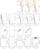 |
Fig. A.1 continued. |
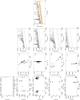 |
Fig. A.1 continued. |
 |
Fig. A.1 continued. |
 |
Fig. B.1 First column: RV versus time of a simulated equatorial spot covering 1.5% of the visible surface and a temperature contrast of 1200 K, for a seen edge-on sun-like star and for five different values of vsini from the upper panels to the lower panels: 3 km s-1, 10 km s-1, 30 km s-1, 50 km s-1, 80 km s-1. Second column: same for the bissectors. Third column: BVS versus RV. Fourth column: BVS versus time. |
 |
Fig. B.2 Same as Fig. 10 for an inclination of 30 degrees (three first lines) and 5 degrees (three last lines), a colatitude (from the pole) of 30 degrees (except 5th line with a colatitude of 60 degrees), and vsini (from upper panels to lower panels) of 3, 10, 40, 10, 10, and 10 km s-1. |
We did not apply any correction factor to the obtained index, as is sometimes done, to calibrate the values with those of Mount Wilson, because 1) we are mainly interested here in relative variations; and 2) such corrections are possible only when a lot of values (for several targets, with stable levels of activity), taken both at Mount Wilson and in the other observing site, are available. Here, we are possibly dealing with a strong variability, so a correction could only be applied if we had simulatenous measurements, for the same targets. Our  ) are similar within 0.3 dex with those already published ones, however.
Acknowledgments
We acknowledge support from the French CNRS and from the Agence Nationale de la Recherche (ANRBLANC10-0504.01). We are grateful to the ESO staff for their help during the observations and to the Programme National de Planétologie (PNP, INSU). These results have made use of the SIMBAD astronomical database, operated at the Centre de Données Astronomiques de Strasbourg, France, and NASAs Astrophysics Data System. We also thank Gérard Zins and Sylvain Cètre for their help in implementing the SAFIR interface.
References
- Aigrain, S., Pont, F., & Zucker, S. 2012, MNRAS, 419, 3147 [NASA ADS] [CrossRef] [Google Scholar]
- Bailey, III, J. I., White, R. J., Blake, C. H., et al. 2012, ApJ, 749, 16 [NASA ADS] [CrossRef] [Google Scholar]
- Berdyugina, S. V. 2005, Liv. Rev. Sol. Phys., 2, 8 [Google Scholar]
- Beuzit, J.-L., Feldt, M., Dohlen, K., et al. 2008, in SPIE Conf. Ser., 7014, 41 [Google Scholar]
- Biller, B. A., Liu, M. C., Wahhaj, Z., et al. 2010, ApJ, 720, L82 [NASA ADS] [CrossRef] [Google Scholar]
- Boisse, I., Moutou, C., Vidal-Madjar, A., et al. 2009, A&A, 495, 959 [NASA ADS] [CrossRef] [EDP Sciences] [Google Scholar]
- Boisse, I., Bouchy, F., Hébrard, G., et al. 2011, A&A, 528, A4 [NASA ADS] [CrossRef] [EDP Sciences] [Google Scholar]
- Borgniet, S., Lagrange, A.-M., Boisse, I., et al. 2013, A&A, submitted [Google Scholar]
- Buenzli, E., Thalmann, C., Vigan, A., et al. 2010, A&A, 524, L1 [NASA ADS] [CrossRef] [EDP Sciences] [Google Scholar]
- Chelli, A. 2000, A&A, 358, L59 [NASA ADS] [Google Scholar]
- Chiang, E., Kite, E., Kalas, P., Graham, J. R., & Clampin, M. 2009, ApJ, 693, 734 [Google Scholar]
- Crockett, C. J., Mahmud, N. I., Prato, L., et al. 2012, ApJ, 761, 164 [NASA ADS] [CrossRef] [Google Scholar]
- Desidera, S., Covino, E., Messina, S., et al. 2011, A&A, 529, A54 [NASA ADS] [CrossRef] [EDP Sciences] [Google Scholar]
- Desort, M., Lagrange, A.-M., Galland, F., Udry, S., & Mayor, M. 2007, A&A, 473, 983 [NASA ADS] [CrossRef] [EDP Sciences] [Google Scholar]
- Dumusque, X., Lovis, C., Ségransan, D., et al. 2011, A&A, 535, A55 [NASA ADS] [CrossRef] [EDP Sciences] [Google Scholar]
- Duncan, D. K., Vaughan, A. H., Wilson, O. C., et al. 1991, ApJS, 76, 383 [NASA ADS] [CrossRef] [Google Scholar]
- Figueira, P., Marmier, M., Bonfils, X., et al. 2010, A&A, 513, L8 [NASA ADS] [CrossRef] [EDP Sciences] [Google Scholar]
- Frankowski, A., Jancart, S., & Jorissen, A. 2007, A&A, 464, 377 [NASA ADS] [CrossRef] [EDP Sciences] [Google Scholar]
- Galland, F., Lagrange, A.-M., Udry, S., et al. 2005, A&A, 443, 337 [NASA ADS] [CrossRef] [EDP Sciences] [Google Scholar]
- García-Alvarez, D., Lanza, A. F., Messina, S., et al. 2011, A&A, 533, A30 [NASA ADS] [CrossRef] [EDP Sciences] [Google Scholar]
- Hernán-Obispo, M., Gálvez-Ortiz, M. C., Anglada-Escudé, G., et al. 2010, A&A, 512, A45 [NASA ADS] [CrossRef] [EDP Sciences] [Google Scholar]
- Hines, D. C., Schneider, G., Hollenbach, D., et al. 2007, ApJ, 671, L165 [NASA ADS] [CrossRef] [Google Scholar]
- Isaacson, H., & Fischer, D. 2010, ApJ, 725, 875 [NASA ADS] [CrossRef] [Google Scholar]
- Janson, M., Carson, J. C., Lafrenière, D., et al. 2012, ApJ, 747, 116 [NASA ADS] [CrossRef] [Google Scholar]
- Kalas, P., Graham, J. R., & Clampin, M. 2005, Nature, 435, 1067 [NASA ADS] [CrossRef] [PubMed] [Google Scholar]
- Kalas, P., Graham, J. R., Chiang, E., et al. 2008, Science, 322, 1345 [NASA ADS] [CrossRef] [PubMed] [Google Scholar]
- Kalas, P., Fitzgerald, M. P., Papadopoulos, P. P., et al. 2010, in Am. Astron. Soc. Meeting Abstracts 215, 42, 377.07 [Google Scholar]
- Lagrange, A.-M., Backman, D. E., & Artymowicz, P. 2000, Protostars and Planets IV, 639 [Google Scholar]
- Lagrange, A.-M., Desort, M., Galland, F., Udry, S., & Mayor, M. 2009a, A&A, 495, 335 [NASA ADS] [CrossRef] [EDP Sciences] [Google Scholar]
- Lagrange, A.-M., Gratadour, D., Chauvin, G., et al. 2009b, A&A, 493, L21 [NASA ADS] [CrossRef] [EDP Sciences] [Google Scholar]
- Lagrange, A.-M., Bonnefoy, M., Chauvin, G., et al. 2010, Science, 329, 57 [NASA ADS] [CrossRef] [PubMed] [Google Scholar]
- Lagrange, A.-M., De Bondt, K., Meunier, N., et al. 2012, A&A, 542, A18 [NASA ADS] [CrossRef] [EDP Sciences] [Google Scholar]
- Lanza, A. F., Boisse, I., Bouchy, F., Bonomo, A. S., & Moutou, C. 2011, A&A, 533, A44 [NASA ADS] [CrossRef] [EDP Sciences] [Google Scholar]
- Lebreton, J., Augereau, J.-C., Thi, W.-F., et al. 2012, A&A, 539, A17 [NASA ADS] [CrossRef] [EDP Sciences] [Google Scholar]
- Lebreton, J., van Lieshout, R., Augereau, J., et al. 2013, A&A, 555, A146 [NASA ADS] [CrossRef] [EDP Sciences] [Google Scholar]
- Lockwood, G. W., Skiff, B. A., Henry, G. W., et al. 2007, ApJS, 171, 260 [NASA ADS] [CrossRef] [Google Scholar]
- Macintosh, B. A., Graham, J. R., Palmer, D. W., et al. 2008, in SPIE Conf. Ser., 7015 [Google Scholar]
- Marois, C., Macintosh, B., Barman, T., et al. 2008, Science, 322, 1348 [NASA ADS] [CrossRef] [PubMed] [Google Scholar]
- Marois, C., Zuckerman, B., Konopacky, Q. M., Macintosh, B., & Barman, T. 2010, Nature, 468, 1080 [NASA ADS] [CrossRef] [PubMed] [Google Scholar]
- Mayor, M., Marmier, M., Lovis, C., et al. 2011, A&A, submitted [arXiv:1109.2497] [Google Scholar]
- Mayor, M., Pepe, F., Queloz, D., et al. 2003, The Messenger, 114, 20 [NASA ADS] [Google Scholar]
- Mesa, D., Gratton, R., Berton, A., et al. 2011, A&A, 529, A131 [NASA ADS] [CrossRef] [EDP Sciences] [Google Scholar]
- Meunier, N., & Lagrange, A.-M. 2013, A&A, 551, A101 [NASA ADS] [CrossRef] [EDP Sciences] [Google Scholar]
- Meunier, N., Lagrange, A.-M., & De Bondt, K. 2012, A&A, 545, A87 [NASA ADS] [CrossRef] [EDP Sciences] [Google Scholar]
- Moór, A., Ábrahám, P., Derekas, A., et al. 2006, ApJ, 644, 525 [NASA ADS] [CrossRef] [Google Scholar]
- Patience, J., Bulger, J., King, R. R., et al. 2011, A&A, 531, L17 [NASA ADS] [CrossRef] [EDP Sciences] [Google Scholar]
- Paulson, D. B., & Yelda, S. 2006, PASP, 118, 706 [NASA ADS] [CrossRef] [Google Scholar]
- Paulson, D. B., Cochran, W. D., & Hatzes, A. P. 2004, AJ, 127, 3579 [Google Scholar]
- Rameau, J., Chauvin, G., Lagrange, A.-M., et al. 2013, A&A, 553, A60 [NASA ADS] [CrossRef] [EDP Sciences] [Google Scholar]
- Rhee, J. H., Song, I., Zuckerman, B., & McElwain, M. 2007, ApJ, 660, 1556 [NASA ADS] [CrossRef] [MathSciNet] [Google Scholar]
- Rodriguez, D. R., & Zuckerman, B. 2012, ApJ, 745, 147 [NASA ADS] [CrossRef] [Google Scholar]
- Santos, N. C., Gomes da Silva, J., Lovis, C., & Melo, C. 2010, A&A, 511, A54 [NASA ADS] [CrossRef] [EDP Sciences] [Google Scholar]
- Schneider, G., Silverstone, M. D., Hines, D. C., et al. 2006, ApJ, 650, 414 [NASA ADS] [CrossRef] [Google Scholar]
- Schröder, C., Reiners, A., & Schmitt, J. H. M. M. 2009, A&A, 493, 1099 [NASA ADS] [CrossRef] [EDP Sciences] [Google Scholar]
- Setiawan, J., Weise, P., Henning, T., et al. 2007, ApJ, 660, L145 [NASA ADS] [CrossRef] [Google Scholar]
- Setiawan, J., Henning, T., Launhardt, R., et al. 2008, Nature, 451, 38 [NASA ADS] [CrossRef] [PubMed] [Google Scholar]
- Sozzetti, A. 2011, in EAS Pub. Ser., 45, 273 [Google Scholar]
- Torres, C. A. O., Quast, G. R., Melo, C. H. F., & Sterzik, M. F. 2008, Young Nearby Loose Associations, ed. B. Reipurth, ASP Monograph publication, 5, 757 [Google Scholar]
- Weise, P., Launhardt, R., Setiawan, J., & Henning, T. 2010, A&A, 517, A88 [NASA ADS] [CrossRef] [EDP Sciences] [Google Scholar]
- Zuckerman, B., & Song, I. 2004, ARA&A, 42, 685 [NASA ADS] [CrossRef] [MathSciNet] [Google Scholar]
- Zuckerman, B., Song, I., Bessell, M. S., & Webb, R. A. 2001, ApJ, 562, L87 [NASA ADS] [CrossRef] [Google Scholar]
All Tables
All Figures
|
Fig. 1 Upper panels: RV versus time, bisectors, BVS versus time and BVS versus RV for the active G-type star HD 183414. In the last panel, we indicate the slope of the (RV, BVS) correlation. Lower panels: same for the pulsating A-type star HD 216956. |
| In the text | |
|
Fig. 2 Upper panels: RV versus time, periodogram of RV and detection limits (from left to right) for the G2V star HD 183414, covering a time span of 189 days. The detection limits have been computed using the rms-based method (black line), LPA (orange stars). Lower panels: same for the A5V star HD 39060 covering a time span of 2600 days. |
| In the text | |
|
Fig. 3 Upper panel: jitter versus age for our stars with enough data points (except HD 177171), for G-K stars (blue diamonds), F-type stars (green triangles), and A-type stars (red squares). An age of 300 Myr was assumed for Fomalhaut. Bottom panel: same for vsini versus age. |
| In the text | |
|
Fig. 4 Upper panel: high-frequency variations of RV for HD 39060 (exposure time of 90 s). Middle panel: same for HD 216956 (exposure time of 8 s). Lower panel: same for HD 218396 (exposure time of 40 s). |
| In the text | |
|
Fig. 5 From left to right: RV variations of HD 105690, bisectors, bisector velocity span (BVS) versus time and BVS versus RV. In the (RV, BVS) diagram, the data corresponding to the period from JD 2 454 343 to JD 2 454 348 are in red. |
| In the text | |
|
Fig. 6 From left to right: RV variations of HD 174429, bisectors, bisector velocity span (BVS) versus time and BVS versus RV. |
| In the text | |
|
Fig. 7 Impact of data averaging on pulsating stars: rms-based detection limits obtained on HD 216956 when using all measurements directly (left panel), and when averaging the data over two days (right panel). Same symbols as for the middle panels of Fig. A.1. |
| In the text | |
|
Fig. 8 Upper panel: LPA detection limits after correction of the RV using the (BVS, RV) slope (blue dots), and after fitting and removing the spot signal (red diamonds), for HD 141943 (jitter = 235 m/s, vsini = 35 km s-1). The uncorrected LPA detection limits are indicated by green crosses. Middle panel: same for HD 183414 (jitter = 67 m/s, vsini = 11.1 km s-1). Lower panel: same for HD 181327 (jitter = 15 m/s, vsini = 17.9 km s-1). |
| In the text | |
|
Fig. 9 Left panel: AO detection limits (observed NaCo limits in plain lines and expected SPHERE limits in dotted lines) and Harps RV detection limits for the active G-type star HD 183414 (192 Myr, 35 pc and timespan of 189 days). In both cases, different star inclinations: 10 (light blue), 30 (red), 60 (blue), and 80 degrees (green) are considered. The Gaia detection limits are also indicated. Middle panel: the same for for the less active F6 star HD 181327 (12 Myr, 51 pc and timespan of 588 days). Right panel: same for the pulsating A-type star HD 188228 (40 Myr, 32 pc and timespan of 1984 days). Since the star is brighter than V = 6, no Gaia data will be available for this star. |
| In the text | |
|
Fig. A.1 From left to right: 1) RV time series. 2) (RV, BVS) diagramme. The slope of the (RV, BVS) correlation is indicated. In a few cases, the value is obviously impacted by a single deviating data point. 3) rms-based detection limits with a 99.8% probability (solid black curve) and a 68.2% probability (dotted curve), achievable limits with a perfect sampling (black solid straight line) and achievable limits if the signal was limited only by photon and instrumental noises and with a perfect temporal sampling (dotted straight lines). The vertical lines in the (period, detection limit) diagramme indicate the timespan for each star. 4) detection limits obtained with the LPA method. “r” indicates the factor of improvement between the LPA and rms-based detection limits. |
| In the text | |
|
Fig. A.1 continued. |
| In the text | |
|
Fig. A.1 continued. |
| In the text | |
|
Fig. A.1 continued. |
| In the text | |
|
Fig. A.1 continued. |
| In the text | |
|
Fig. A.1 continued. |
| In the text | |
|
Fig. B.1 First column: RV versus time of a simulated equatorial spot covering 1.5% of the visible surface and a temperature contrast of 1200 K, for a seen edge-on sun-like star and for five different values of vsini from the upper panels to the lower panels: 3 km s-1, 10 km s-1, 30 km s-1, 50 km s-1, 80 km s-1. Second column: same for the bissectors. Third column: BVS versus RV. Fourth column: BVS versus time. |
| In the text | |
|
Fig. B.2 Same as Fig. 10 for an inclination of 30 degrees (three first lines) and 5 degrees (three last lines), a colatitude (from the pole) of 30 degrees (except 5th line with a colatitude of 60 degrees), and vsini (from upper panels to lower panels) of 3, 10, 40, 10, 10, and 10 km s-1. |
| In the text | |
Current usage metrics show cumulative count of Article Views (full-text article views including HTML views, PDF and ePub downloads, according to the available data) and Abstracts Views on Vision4Press platform.
Data correspond to usage on the plateform after 2015. The current usage metrics is available 48-96 hours after online publication and is updated daily on week days.
Initial download of the metrics may take a while.