| Issue |
A&A
Volume 558, October 2013
|
|
|---|---|---|
| Article Number | A74 | |
| Number of page(s) | 9 | |
| Section | Stellar structure and evolution | |
| DOI | https://doi.org/10.1051/0004-6361/201322335 | |
| Published online | 04 October 2013 | |
Swift J053041.9-665426, a new Be/X-ray binary pulsar in the Large Magellanic Cloud⋆
1
Max-Planck-Institut für extraterrestrische Physik,
Giessenbachstraße,
85748
Garching,
Germany
e-mail:
gevas@mpe.mpg.de
2
School of Physics and Astronomy, University of
Southampton, Highfield, Southampton
SO17 1BJ,
UK
Received: 22 July 2013
Accepted: 25 August 2013
Aims. We observed the newly discovered X-ray source Swift J053041.9-665426in the X-ray and optical regime to confirm its proposed nature as a high mass X-ray binary.
Methods. We obtained XMM-Newton and Swift X-ray data, along with optical observations with the ESO Faint Object Spectrograph, to investigate the spectral and temporal characteristics of Swift J053041.9-665426.
Results. The XMM-Newton data show coherent X-ray pulsations with a period of 28.77521(10) s (1σ). The X-ray spectrum can be modelled by an absorbed power law with photon index within the range 0.76 to 0.87. The addition of a black body component increases the quality of the fit but also leads to strong dependences of the photon index, black-body temperature and absorption column density. We identified the only optical counterpart within the error circle of XMM-Newton at an angular distance of ~0.8′′, which is 2MASS J05304215-6654303. We performed optical spectroscopy from which we classify the companion as a B0-1.5Ve star.
Conclusions. The X-ray pulsations and long-term variability, as well as the properties of the optical counterpart, confirm that Swift J053041.9-665426 is a new Be/X-ray binary pulsar in the Large Magellanic Cloud.
Key words: galaxies: individual: Large Magellanic Cloud / X-rays: binaries / stars: emission-line, Be / stars: neutron / pulsars: individual: Swift J053041.9-665426
© ESO, 2013
1. Introduction
Be/X-ray binaries (BeXRBs) are a subclass of high mass X-ray binaries (HMXRBs). The binary consists of a compact object, typically a neutron star, that accretes mass from a high-mass main sequence, subgiant or giant OBe star. Currently, there are no confirmed black hole BeXRB systems (Belczynski & Ziolkowski 2009). The optical companions in BeXRBs are rapidly rotating emission-line stars, typically having spectral classes between O5 and B9 (Coe et al. 2005). The rapidly rotating high mass star loses material resulting in the formation of an equatorial disc, which is also referred to as decretion disc. The exact mechanism by which material is fed by the star to the disc is not yet well understood (Porter & Rivinius 2003). This disc is responsible for the optical emission lines, mainly the Balmer and Paschen series of Hydrogen and sometimes He and Fe lines. Another signature of these systems is the infrared (IR) excess also originating from the equatorial disc (for a full review see Reig 2011).
In a BeXRB system the neutron star is usually orbiting its companion in a significantly eccentric orbit that may be inclined to the decretion disc (Townsend et al. 2011). This results in higher accretion rates when the stellar separation is smaller and/or the neutron star passes through the decretion disc, which can lead to the X-ray emission being transient in nature. During these phases of enhanced accretion the X-ray luminosity can reach values up to 1036−37 erg s-1. These so called Type I outbursts can be identified from their periodic behaviour related to the orbital period of the binary system. Sometimes, giant outbursts (Type II) may occur at luminosities greater than 1037 erg s-1 and last for several orbital periods. These are believed to be caused by large structural changes in the decretion disc which can be completely lost and replenished (Okazaki et al. 2013).
The strong magnetic field of the neutron star funnels mass accretion onto the magnetic poles and leads to the formation of an accretion column. Shocks heat the gas which then emits X-rays (for a detailed review of the emission mechanisms see Hickox et al. 2004; Frank et al. 2002). Due to the localised mass accretion onto the magnetic poles of the rotating neutron star, it is possible to detect pulses in the X-ray light curve. The pulse profiles can be single peaked, double peaked or even more complex depending on the accretion geometry and viewing angle (Annala & Poutanen 2010).
In the last decade, a thermal soft excess has been detected in several BeXRB pulsars. It has been suggested that the presence of a soft spectral component could be a very common feature intrinsic to X-ray pulsars. Hickox et al. (2004) concluded that the origin of this excess could be related to the total luminosity of the source. For sources with higher luminosity (LX > 1038 erg s-1) the excess could be explained only by reprocessing of hard X-rays from the neutron star by optically thick accreting material. In less luminous sources (LX < 1036 erg s-1), the soft excess can be due to emission by photoionised or collisionally heated gas or thermal emission from the surface of the neutron star. Either or both of these types of emission can be present for sources with intermediate luminosity.
The study of BeXRBs in nearby galaxies can provide us with more complete and homogeneous samples of BeXRB populations with the advantage of low foreground absorption and well known distances compared to sources in our Galaxy. The Magellanic Clouds are the closest star-forming galaxies to our own, making them ideal for the study of their X-ray binary populations. Approximately 60 confirmed pulsars have been found in the Small Magellanic Cloud (SMC) so far (Haberl & Pietsch 2004; Coe et al. 2005, 2010), and 45 candidates have been identified during the recent XMM-Newton survey of the SMC (Sturm et al. 2013; Haberl et al. 2012). On the other hand the Large Magellanic Cloud (LMC), which is 10 times more massive than the SMC, has only 15 confirmed BeXRBs (Maggi et al. 2013). A possible explanation is the connection between the density of BeXRBs and the recent star formation of the galaxy. Antoniou et al. (2010) found a correlation between the SMC BeXRB population and the recent star formation ~(25−60) Myr ago. For the LMC a similar correlation has been reported but for stellar populations with ages ~(15−50) Myr (Antoniou et al. 2011). The most recent star-formation episodes in the LMC occurred 12 and 100 Myr ago (Harris & Zaritsky 2009). The X-ray coverage of the LMC is not nearly as complete as that of the SMC and so early interpretations on the connection between star-formation rate and its BeXRB population would be dubious. The XMM-Newton survey of the LMC (PI: F. Haberl) will achieve a homogeneous coverage of the inner ~4.5° × 4.5° region of the LMC and will provide us with a more complete BeXRB sample of this region.
In this work we report on a newly discovered BeXRB in the LMC, Swift J053041.9-665426. The source was discovered on 2011 Nov. 6 during a Swift observation of the LMC nova 2009B (Sturm et al. 2011a). It was then detected in a subsequent Swift follow-up observation that yielded an improved position and X-ray spectrum (Sturm et al. 2011b). Based on its spectral properties and the correlation with an early-type optical counterpart the source was characterised as a BeXRB candidate. Variability of the optical counterpart has been reported (Charles et al. 2011), which is consistent with such a classification. In addition to the existing Swift observations we present the spectral and timing analysis of an XMM-Newton target-of-opportunity (ToO) observation as well as the results of optical spectroscopy performed on its companion.
2. Observations and data reduction
2.1. X-ray observations
For the current analysis we used six Swift, one XMM-Newton and one ROSAT observations of the field surrounding the source. The detailed observation log is recorded in Table 1.
X-ray observations of Swift J053041.9-665426.
The source was detected in four more Swift observations of the field in addition to those reported above. For the spectral extraction we used the HEASoft1 task xselect and an extraction region with radius 35′′ for the source and 300′′ for the background.
Following the detection of Swift J053041.9-665426in the Swift observation on 2012 Aug. 28, we obtained an XMM-Newton ToO observation (PI: P. Maggi). The observation was performed on 2012 Sep. 03 and allowed us to detect the source during outburst. The source was located on-axis, on CCD4 of the EPIC-pn (Strüder et al. 2001) and on CCD1 of the EPIC-MOS (Turner et al. 2001) detectors. XMM-Newton SAS 12.0.12 was used for data processing. The observation was affected by high background for the first 10 ks, which then stayed at a moderate level for the rest of the exposure. We used a background threshold of 16 and 8 counts ks-1 arcmin-2 for the EPIC-pn and EPIC-MOS detectors respectively which resulted in net exposure times of 22.3/26.0/26.0 ks for EPIC-pn/MOS1/MOS2 after flare removal. The source event extraction was performed using a circle around the source, while the background events were extracted from a point-source free area on the same CCD but with different pixel columns for EPIC-pn. We optimised the size of the source extraction area using the SAS task eregionanalyse. The final values used for the extraction are given in Table 1, which summarises the available X-ray observations. For the EPIC-pn spectra and light curves, we selected single-pixel and double-pixel events (PATTERN ≤ 4), while in the case of EPIC-MOS we used single to quadruple events (PATTERN≤12). The quality flag FLAG = 0 was used throughout. The SAS task especget was used to create the spectra for the spectral analysis. The spectra were binned to achieve a minimum signal-to-noise ratio of five for each bin. This allows the use of the χ2 statistics in the spectral analysis, which was performed with XSPEC (Arnaud 1996) version 12.7.0.
A ROSAT archival pointed observation covering the position of Swift J053041.9-665426is also available, which we used to establish an upper limit for the source luminosity.
2.2. Optical spectroscopy
The optical data were taken with the ESO Faint Object Spectrograph and Camera (EFOSC2) mounted at the Nasmyth B focus of the 3.6 m New Technology Telescope (NTT), La Silla, Chile on the nights of 2011 Dec. 8−10. A slit width of 1.5′′ was used, along with Grisms 14 and 20 for blue and red end spectroscopy, respectively. For details on the individual Grisms see Table 2. Filter OG530 was used in conjunction with Grism 20 to block second order effects. The resulting spectra were recorded on a Loral/Lesser, thinned, AR-coated, UV flooded, MPP CCD with 2048 × 2048 pixels. Wavelength calibration was achieved using comparison spectra of helium and argon lamps taken throughout the observing run with the same instrument configuration. The data were reduced using the standard packages available in the Image Reduction and Analysis Facility (IRAF)3. The spectra were normalised to remove the continuum and a redshift correction was applied corresponding to the recession velocity of the LMC (−280 km s-1, Richter et al. 1987).
ESO Faint Object Spectrograph grism information.
3. X-ray data analysis and results
3.1. X-ray position
X-ray images were created from all the EPIC cameras using the XMM-Newton standard energy sub-bands (Watson et al. 2009). Source detection was performed simultaneously on all the images using the SAS task edetect_chain. Boresight correction was performed on the images based on the position of three identified background X-ray sources in the same field. The positional correction based on these sources was found to be ~1′′. The source position was determined to RA = 05h30m42 17 and Dec = –66°54′31
 0 (J2000.0) with a 1σ statistical uncertainty of 0.08′′. The total 1σ positional uncertainty, however, is determined by the remaining systematic uncertainty assumed to be 0.5′′ (see Sect. 4.3 of Sturm et al. 2013).
3.2. Spectral analysis
All the EPIC spectra were fitted simultaneously for the same model parameters with an additional scaling factor to account for instrumental differences. For the EPIC-pn we fixed the scaling factor to be 1, while for both EPIC-MOS we obtained values of CMOS = 1.08 ± 0.05, which is consistent with the expected value, as EPIC-MOS is known to provide ~5% higher fluxes than EPIC-pn (see Stuhlinger et al. 2006, or the latest version of the XMM-Newton calibration manual4). The photoelectric absorption was modelled as a combination of Galactic foreground absorption and an additional column density accounting for both the interstellar medium of the LMC and the intrinsic absorption by the source. The Galactic photoelectric absorption was set to a column density of NH,GAL = 5.86 × 1020 cm-2 (Dickey & Lockman 1990) with abundances according to Wilms et al. (2000). The additional column density NH,LMC was left as a free parameter with abundances of 0.49 for elements heavier than helium (Rolleston et al. 2002). All the uncertainties were calculated based on a Δχ2 statistic of 2.706, equivalent to a 90% confidence level for one parameter of interest.
The spectra were fitted by an absorbed power law, resulting in an acceptable fit with reduced χ2 value of  . However, we found systematic deviations in the residuals. Therefore, we further tested the spectra for the existence of additional features typically shown by BeXRBs. The best fit was achieved by an absorbed power law plus a black body that contributes to the soft part of the spectrum. The two-component model significantly improves the fit over the simple power-law (
 vs. 1.4 for two additional parameters), with the F-test probability for the additional black-body component being ~8 × 10-21. The black-body component accounts for 53.8% of the detected flux and demonstrates model dependent uncertainties on the photon index of the power-law model. The black-body model bbodyrad uses a normalisation proportional to the emission area (norm
  , where Rkm denotes the emission radius in km and D10 the source distance in units of 10 kpc). From this relation we derived a radius for the emission region of ~800 m. This area should be indicative of the size of the accretion column from which the black-body radiation is believed to originate (Hickox et al. 2004). The spectra together with the best-fit power-law and black-body model are presented in Fig. 1, where we also compare the residuals with those of the simple power-law model fit.
It should be noted that although the addition of the black-body model improves the quality of the fit it also adds large uncertainties to the best-fit values. Thus different combinations of parameters can actually provide a similarly good fit (see Fig. 2). Softer power-laws (higher Γ, where Γ is defined as the index in a power low spectrum A(E) ∝ E− Γ) can be compensated with higher absorption values, while for lower Γ the best fit model gives lower absorption values and lower black-body temperature. Therefore, for any constant value of Γ between 0 and 0.8 the reduced Δχ2 for the fit varies only marginally around one. Also by looking at Fig. 1, we can see that the black-body component contributes almost to all the emission below 6 keV. Because of the large uncertainties, we present another more consistent set of parameters for a fixed photon index at the value of 0.7, which is close to the one found with the single power-law fitting. The best-fit results are listed in Table 3.
Replacing the black-body component by alternative models such as, a Comptonisation spectrum, a thermal bremsstrahlung or a MEKAL thermal plasma only gives a marginal improvement of the fit compared to the single power-law model. The only models that showed similar goodness of fit were a power-law with high-energy exponential cutoff (cutoffpl in xspec, with Γ = −0.68 and e-folding energy of 2.8 keV) and the broken power-law (bknpower in xspec, with Γ1 = 0.1, Γ2 = 1.2, break at 3.3 keV). However, we do not expect negative photon indices nor a break at such low energies for BeXRB systems.
Individual Swift observations did not provide sufficient statistics to determine spectral parameters independently, but using a group of them to simultaneously fit a model provided better statistics. For the first four observations that were taken during the same outburst and were at similar flux level we performed the event extraction as described in Sect. 2.1 and performed a simultaneous spectral fitting with XSPEC. Due to lower statistics compared to the XMM-Newton spectra we only tested an absorbed power-law model. The best-fit values are also listed in Table 3. For the two Swift observations taken in 2012 we used the best-fit parameters for the absorbed power-law model as obtained from the XMM-Newton spectrum (near in time) and derived the fluxes of these Swift observations by adjusting the normalisation.
From the ROSAT observation we estimated an upper limit for the X-ray flux assuming the same spectral properties as in the XMM-Newton detection and assuming that for a detection at least seven counts are needed for an on-axis observation.
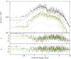 |
Fig. 1 EPIC spectra of Swift J053041.9-665426. The top panel shows the EPIC-pn (black), EPIC-MOS1 (red) and EPIC-MOS2 (green) spectra, together with the best-fit model (solid line) of an absorbed power-law (dotted line) plus a black-body (dash-dotted line). The residuals for this model are plotted below (bottom panel), while for comparison the best-fit single power-law model residuals are also plotted (middle panel). |
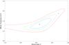 |
Fig. 2 Photon index Γ vs. temperature kT (keV) confidence contours for the power-law + black-body model. Confidence levels of 1, 2 and 3σ are shown in blue green and red. The star represent the best-fit values, while the diamond marks the best fit for a fixed Γ of 0.7. |
Spectral fit results.
3.3. X-ray long-term variability
To study the long-term variability of Swift J053041.9-665426, we estimated the flux level for all available observations (see Table 1). The source flux from the XMM-Newton ToO observation was determined from the spectra as described in Sect. 3.2. We transformed the observed fluxes to unabsorbed luminosities based on a LMC distance of 50 kpc. The net count rates and unabsorbed luminosities are given in Table 1.
The Swift observations indicate a variability of up to a factor of ~14. The XMM-Newton ToO observation yields a luminosity lower than any Swift observation giving a total variability of ~23. The upper limit derived from the ROSAT observation is ~1.6 times smaller than the XMM-Newton detected flux, providing evidence for even larger variability. However, the photoelectric absorption will have large effect on the soft ROSAT energy band and may introduce large systematic uncertainties.
3.4. Timing analysis
We corrected the XMM-Newton EPIC event arrival times to the solar-system barycentre using the SAS task barycen. The X-ray light curves were searched for periodicities using fast Fourier transform (FFT) and light curve folding techniques. The power density spectra derived from time series in various energy bands from all three EPIC instruments show a periodic signal at ω ~ 0.0347521 Hz. To increase the signal-to-noise ratio, we then created time series from the merged event list of EPIC-pn and EPIC-MOS (delimited to common good time intervals). Figure 3 shows the inferred power density spectrum from the (0.2−10) keV energy band with a strong peak at a frequency of 0.0347520(5) Hz. Following Haberl et al. (2008) we used a Bayesian periodic signal detection method (Gregory & Loredo 1996) to determine the pulse period with 1σ uncertainty to (28.77521 ± 0.00010) s. The period folded pulse profiles in the EPIC standard energy bands together with the hardness ratios derived from the pulse profiles in two adjacent energy bands (HRi = (Ri + 1 − Ri)/(Ri + 1 + Ri) with Ri denoting the background-subtracted count rate in energy band i) are plotted in Fig. 4. To achieve better statistics, the first two standard energy bands were combined in the top panel, the bottom panel shows all five energy bands combined. All the profiles are background-subtracted and normalised to the average count rate (0.0215, 0.0813, 0.1403, 0.0950, and 0.3388 cts s-1, from top to bottom).
4. Analysis and results of optical data
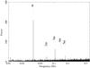 |
Fig. 3 Power density spectrum created from the merged EPIC-pn and EPIC-MOS data in the (0.2−10.0) keV energy band. The time binning of the input light curve is 0.8156671 s. On the plot we can see the best-fit frequency of ω = 0.034752 Hz and its first, second and fourth harmonics. |
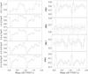 |
Fig. 4 Left: pulse profiles obtained from the merged EPIC data in different energy bands. Right: hardness ratios as a function of pulse phase derived from the pulse profiles in two neighbouring standard energy bands. |
4.1. Optical counterpart
The most precise X-ray position of Swift J053041.9-665426was derived from XMM-Newton data (Sect. 2.1). Within the 3σ error circle we found only one candidate counterpart at a distance of ~0.8′′. The object was identified in 2MASS (Skrutskie et al. 2006; Cutri et al. 2003), IRSF (Kato et al. 2007) and MCPS (Zaritsky et al. 2004) catalogs and the WISE All-sky data release. It is listed as J05304215-6654303 in the 2MASS catalogue. The various magnitudes are summarised in Table 4.
A finding chart of Swift J053041.9-665426is shown in Fig. 5. The image was obtained with ESO NTT during the spectroscopic observation of the source and the image coordinates were corrected based on the 2MASS catalogue with a positional uncertainty ~0.2′′.
The spectral energy distribution (SED) of Be stars consists of two components (Dougherty et al. 1994), the emission from the surface of the star (stellar atmosphere of T ~ (18 000−38 000) K) and an infrared excess from the equatorial disc. Due to the evolution of the disc with time the luminosity of the system may vary. Therefore, simultaneous measurements of individual colours are needed for a meaningful SED. From the available data it is not possible to construct an SED and compare it with available models. However, we see evidences for variability of the optical counterpart, which is typical for BeXRB systems.
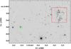 |
Fig. 5 Finding chart of Swift J053041.9-665426. The image was taken with ESO NTT (V#641 filter) during the spectroscopic observation of the source. The green error circle with radius of 1.6′′ translates to the 3σXMM-Newton positional uncertainty. On the right part of the image at a distance of 0.95′ from the XMM-Newton position of Swift J053041.9-665426the nearby star cluster KMHK 987 is seen (dashed red box). |
Optical and IR photometry of Swift J053041.9-665426.
The optical counterpart of Swift J053041.9-665426was also found in the Spitzer SAGE catalogs of the Magellanic Clouds (Meixner et al. 2006). Using the J colours from various surveys and the IRAC 3.6, 4.5, 5.8 μm colours (see Table 4) and based on the analysis of Bonanos et al. (2009, 2010) we determined the position of the source on the JIRSF vs. JIRSF−[3.6], JIRSF vs. JIRSF−[5.8], JIRSF vs. JIRSF−[8.0] diagrams. Most of the B stars have a J−[3.6] colour ~[−0.2:0.2] mag. While, depending on the four available observations in the J filter, the optical counterpart of Swift J053041.9-665426has a larger colour index between 0.7 and 1.26 mag. Based on that we clearly detect infrared excess of the counterpart of Swift J053041.9-665426. This excess can be attributed to the free-free emission from the disc around the star.
4.2. Spectral classification
From the optical spectroscopy we clearly see Hα emission from the proposed counterpart of Swift J053041.9-665426. Figure 6 shows the red end of the spectrum taken on 2011 Dec. 10. The Hα equivalent width, considered as an indicator for circumstellar disc size (Stevens et al. 1997), is − (16.8 ± 0.9) Å.
OB stars in our own Galaxy are classified using the ratio of certain metal and helium lines (Walborn & Fitzpatrick 1990) based on the Morgan-Keenan (Morgan et al. 1943) system. However, in lower metallicity environments such as the Magellanic Clouds this is not possible, due to the absence or weakness of the metal lines. Therefore, the optical spectrum of Swift J053041.9-665426was classified using the method developed by Lennon (1997) for B-type stars in the SMC. The luminosity classification method from Walborn & Fitzpatrick (1990) was assumed in this work.
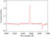 |
Fig. 6 Spectrum of Swift J053041.9-665426in the wavelength range λ6000–7000Å as measured with the NTT on 2011-12-10. The spectrum has been normalised to remove the continuum and redshifted by − 280 km s-1. |
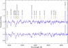 |
Fig. 7 Spectra of Swift J053041.9-665426in the wavelength range λ3900−5000 Å taken on concurrent nights with the NTT. The spectra have been normalised to remove the continuum and redshift corrected by −280 km s-1. Atomic transitions relevant to spectral classification have been marked. The lower one was taken on the first night, while a different normalisation has been used for better representation and comparison. |
Figure 7 shows two unsmoothed optical spectra of Swift J053041.9-665426taken on 2011 Dec. 8 and 9, dominated by the hydrogen Balmer series. The equivalent widths of the Hβ lines are (− 1.3 ± 0.2) Å and (− 1.4 ± 0.2) Å, respectively. The Siiv lines at λ4088,λ4116 Å are both clearly present in both spectra, despite the rotational broadening of the Hδ line, suggesting a classification earlier than B1.5. The Heii line at λ4686 Å is just visible above the noise level of the data, implying a classification of B1. There also appears to be marginal evidence for a line at λ4541 Å (particularly in the lower spectrum) indicating a spectral class of B0.
The luminosity class of the system was determined using the ratios of Si ivλ4088/He i+iiλ4026, Si ivλ4088/He iλ4143, Si ivλ4116/He iλ4121 and He iiλ4686/He iλ4713. The first three increase with increasing luminosity (decreasing luminosity class) and the latter increases with decreasing luminosity (increasing luminosity class). All but the Siivλ4116/Heiλ4121 ratio point to a luminosity class V (the other suggesting a luminosity class III). This is supported by the weak Oii spectrum, characteristic of dwarf stars. The V-band magnitude of the companion star is reported to be (15.32 ± 0.02) mag by Zaritsky et al. (2004). Along with a distance modulus of (18.52 ± 0.07) mag (Bonanos et al. 2011) and an AV of (0.26 ± 0.02) mag calculated using the Galactic column density towards the source of (5.8 ± 0.3) × 1020 cm-2 (Dickey & Lockman 1990) and the results of Güver & Özel (2009), this leads to an absolute magnitude MV = −3.46 ± 0.08 mag, consistent with a B0V star. As such we classify the optical counterpart of Swift J053041.9-665426as a B0-1.5V star.
4.3. MACHO light curve
We identified the optical counterpart in the on-line catalogue5 (photometry id-61:8197:41:64925) of the MAssive Compact Halo Objects (MACHO) project. The MACHO observations were made using the 1.27-m telescope at Mount Stromlo Observatory, Australia. A dichroic beamsplitter and filters provide simultaneous CCD photometry in two passbands, the RMACHO red band (6300−7600 Å) and the BMACHO blue band (4500−6300 Å). The standard MACHO instrumental magnitudes are extracted with SoDoPHOT and are based on point-spread function fitting and differential photometry relative to bright neighbouring stars. SoDoPHOT stands for Son of DoPhot, a revised package based on DoPhot6 algorithms but optimised to MACHO image data. The SoDoPHOT instrumental magnitude is given as 2.5 times the common logarithm of the integrated number of electrons in the fit to the analytical PSF, divided by 100. MACHO light curves may show systematic variations in brightness due to the different air-mass during individual observations. Additionally, artificial “seasonal rolls” (~1 yr periods) may be a result of the target being observed at progressively higher air-masses as the season progresses. Finally instrumental light curves are affected by observations made from either side of the telescope pier (a German equatorial mount). Thus stars will alternatively be located on the CCDs rotated by 180 degrees from each other in the focal plane.
To use the light curves, we need to correct them for the above effects, e.g. the air-mass and the responses of the different CCDs. We followed the analysis of Alcock et al. (1999). In their work they derived corrections for all the instrumental magnitudes based on a statistical analysis of the properties of the detected stars in the MACHO fields of the LMC. But the relations given in their work cannot be applied in a straightforward way to a single star. In particular the coefficients for the air-mass-colour corrections must be derived using separate knowledge of the shape of a light curve (e.g. Eqs. (7) and (8) in Alcock et al. 1999). To correct the instrumental light curve, we searched all the parameter space for these coefficients and derived the best solution for a continuous light curve. Finally we transformed the corrected magnitudes to the Johnson V and Cousins R bands. The complete analysis added a systematic uncertainty of ~0.02 mag to the light curve.
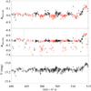 |
Fig. 8 MACHO light curves for a time period of 2541 days: the “blue” BMACHO light curve is plotted on the top panel, the “red” RMACHO in the middle. In both of them red triangles and black stars indicate instrumental magnitudes taken on different pier setup. The corrected Johnson V magnitude is plotted on the bottom panel. |
In Fig. 8 we show the light curves for RMACHO, BMACHO and the corrected Johnson V magnitude. The BMACHO light curve shows evidence for periodicity and both instrumental magnitudes show an outburst at the end of the light curve. The magnitude of the outburst was 0.15 and 0.2 mag in the BMACHO and the RMACHO filter, respectively. The reddening of the source during the outburst is typical of Be star in the phase of growing the circumstellar disc (de Wit et al. 2006). The RMACHO light curve shows several dips up to 0.6 mag, which are more often seen in one of the instrument set-up. These dips are mostly seen during the winter and spring period and might be caused by weather conditions, which affect the RMACHO filter more. Another characteristic of the dips is that they seem to appear more often in observations at low airmass values <1.25. Consequently we believe that these dips are only instrumental artifacts and decided to exclude them from our analysis.
We computed the Lomb-Scargle (LS) periodogram (Scargle 1982) for the light curves of the instrumental magnitudes, excluding the outburst (MJD > 51 150). For BMACHO we found a period of 373 d which could be artificial as the instrument setup changes approximately every 6 months. For the RMACHO we find a period of ~316 d. After correcting the instrumental magnitudes, we get a period of ~390 d for the V-band light curve with a LS power less than 15. The period is still close to one year. In order to test if all the corrections were done accurately, we used the same technique to correct the light curves of other nearby stars. None of the other stars showed a period close to one year or showed a similar light curve. We corrected the light curves of the source by normalising the two data sets obtained by different instrument/pier orientation by their average values, this caused the LS power to fall dramatically. If the period was intrinsic to the sources, we would expect the LS power to rise, not to fall. We would also expect a genuine period to be much more consistent across the different bands. Therefore we conclude that from the light curve we have no clear evidence for the optical period of the optical counterpart of Swift J053041.9-665426, in contrast of what the usage of the uncorrected instrumental data might yield.
5. Discussion
The X-ray fluxes (see Table 1) suggest that Swift J053041.9-665426was detected during an outburst in Nov. 2011, while the XMM-Newton ToO observation was performed at a lower luminosity level. The flux upper limit derived from the ROSAT observation is close to the source luminosity during the XMM-Newton ToO observation, suggesting that the non-detection might be explained by high absorption. However, due to the nature of the source, we cannot rule out the possibility that the source was inactive during the ROSAT observation. There are examples of BeXRBs being inactive for a long period before brightening up again (e.g. SAXJ0103.2-7209, Eger & Haberl 2008).
Knowing that the BeXRB population correlates with star formation regions with ages ~15−50 Myr (Antoniou et al. 2011) it is likely that the system originated from a nearby cluster. Swift J053041.9-665426 is located near the star cluster KMHK 987 at a projected angular distance of 0.95′ (see Fig. 5). KMHK 987 has a radius of 0.48′ and an age of ~31 Myr (Glatt et al. 2010). For the case of HMXRBs in the SMC a convincing link between the binary systems and near star clusters has been reported that leads to an average space velocity of these systems arising from a supernova kick (Coe 2005). Assuming a value of 5 Myr for the most likely maximum lifetime of the Be star after the NS has been formed (Savonije & van den Heuvel 1977) we can estimate a lower limit on the runaway velocity imposed to the system by the supernova kick. In our case this leads to a velocity of 2.6 km s-1. Knowing that the systems true motion has a random direction to our line of sight the true velocity could be much larger. The true velocity given as function of the angle θ between the line of sight and the moving direction of the source is u = 2.6/sinθ km s-1. On a statistical basis this value is lower than the average velocity reported for BeXRB systems in our galaxy (e.g. 19 ± 8 km s-1, van den Heuvel et al. 2000). A simple explanation could be that the value we used for the time since the creation of the binary is arbitrary and could be much lower, or that the system could originate from a more distant cluster. Another close cluster NGC 2002, which is even younger with age ~11 Myr and is found at a distance of 2.55′ (~37 pc). By doing the same calculations on this cluster we derive a lower limit for the runaway velocity of 14 km s-1. Based on the above estimates, Swift J053041.9-665426could originate from either of those two clusters.
The power-law photon index derived from the EPIC spectra of 0.1–0.8 (depending on the model, and the existence of a black-body component) is on the hard side of the distribution of photon indices of BeXRBs, which has a maximum at ~0.9−1.0 (Haberl et al. 2008). A spectral analysis of the available Swift data gives a higher index of 1.7 ± 0.5 (Sturm et al. 2011a) and 1.15 ± 0.17 (Sturm et al. 2011b), but in both cases the statistics are much lower than that in the EPIC observation.
The X-ray spectrum is well described with a combination of a power-law and a thermal black-body component, accounting for ~53% of the flux in the (0.3−10.0) keV band. This soft component has been recently reported in many other BeXRB pulsars (e.g. La Palombara & Mereghetti 2006; Reig et al. 2012). From the parameters of the model, we estimate a black-body radius of ~800 m for the emission region (accretion column). This value agrees with other persistent HMXRBs found in our Galaxy (La Palombara et al. 2013). In fact we can compare the emission region size with the one estimated by the analysis of Hickox et al. (2004). Assuming standard values for the neutron star mass, radius and magnetic field of MNS = 1.4 M⊙, RNS = 106 cm and BNS = 1012 G, and by using the black-body luminosity derived by the fit we get an estimate of ~320 m for the black-body emitting radius. If this description is correct we might expect some variability on the thermal component with the phase of the spin period that could result in a variable hardness ratio. In the pulse profiles of Swift J053041.9-665426we see a significant change in the hardness ratio of the harder bands (HR4). This behaviour has been well studied in Swift J045106.8-694803, another BeXRB in the LMC (Bartlett et al. 2013). Unfortunately, for Swift J053041.9-665426this occurs only for a small time interval and cannot provide good statistics for further investigation of the spectrum.
We note that one should be careful in the interpretation of the two-component model with power-law and black body. Insufficient statistics of the spectral data can lead to strong dependences of the photon index, black-body temperature and absorption column density. For example La Palombara et al. (2009) derive a large negative Γ for RX J1037.5-5647, a known BeXRB pulsar in the Milky Way, when using this model.
Some low strength peaks that are found in the optical periodograms for near one year period can be attributed both to the instrumental setup and weather observing conditions and thus prevent us from deriving a clear periodic behaviour, which could indicate an orbital period.
6. Conclusion
Analysis of the XMM-Newton ToO observation of Swift J053041.9-665426revealed X-ray pulsations at ~28.78 s. The X-ray spectrum is best described by a double component model, composed of an absorbed power-law and black-body. We have spectroscopically classified the optical counterpart as a B0-1.5Ve star. The strong IR signal, combined with the clear evidence for significant Hα emission, points convincingly to the existence of a circumstellar disc as the source of accretion material in the system. The analysis of the optical light curve showed a ~150 d burst, but there is no clear optical period found in the two colour light curves. Our results confirm Swift J053041.9-665426as a BeXRB with a neutron star primary, making it the 16th known BeXRB pulsar in the LMC.
Science Analysis Software (SAS), http://xmm.esac.esa.int/sas/
Image Reduction and Analysis Facility (IRAF), http://iraf.noao.edu/
Acknowledgments
The XMM-Newton project is supported by the Bundesministerium für Wirtschaft und Technologie / Deutsches Zentrum für Luft- und Raumfahrt (BMWi/DLR, FKZ 50 OX 0001) and the Max-Planck Society. We thank the SWIFT team for accepting and carefully scheduling the target of opportunity observations, and we acknowledge the use of public data from the SWIFT data archive. This paper utilizes public domain data obtained by the MACHO Project, jointly funded by the US Department of Energy through the University of California, Lawrence Livermore National Laboratory under contract No. W-7405-Eng-48, by the National Science Foundation through the Center for Particle Astrophysics of the University of California under cooperative agreement AST-8809616, and by the Mount Stromlo and Siding Spring Observatory, part of the Australian National University. G.V., P.M. and R.S. acknowledge support from the BMWi/DLR grant FKZ 50 OR 1208, 1201 and 0907 respectively.
References
- Alcock, C., Allsman, R. A., Alves, D. R., et al. 1999, PASP, 111, 1539 [NASA ADS] [CrossRef] [Google Scholar]
- Annala, M., & Poutanen, J. 2010, A&A, 520, A76 [NASA ADS] [CrossRef] [EDP Sciences] [Google Scholar]
- Antoniou, V., Zezas, A., Hatzidimitriou, D., & Kalogera, V. 2010, ApJ, 716, L140 [NASA ADS] [CrossRef] [Google Scholar]
- Antoniou, V., Zezas, A., & Kalogera, V. 2011, in Am. Astron. Soc. Meet. Abstr. 218, 228.29 [Google Scholar]
- Arnaud, K. A. 1996, in Astronomical Data Analysis Software and Systems V, eds. G. H. Jacoby, & J. Barnes, ASP Conf. Ser., 101, 17 [Google Scholar]
- Bartlett, E. S., Coe, M. J., & Ho, W. C. G. 2013, MNRAS, accepted [Google Scholar]
- Belczynski, K., & Ziolkowski, J. 2009, ApJ, 707, 870 [NASA ADS] [CrossRef] [Google Scholar]
- Bonanos, A. Z., Massa, D. L., Sewilo, M., et al. 2009, AJ, 138, 1003 [NASA ADS] [CrossRef] [Google Scholar]
- Bonanos, A. Z., Lennon, D. J., Köhlinger, F., et al. 2010, AJ, 140, 416 [NASA ADS] [CrossRef] [Google Scholar]
- Bonanos, A. Z., Castro, N., Macri, L. M., & Kudritzki, R.-P. 2011, ApJ, 729, L9 [NASA ADS] [CrossRef] [Google Scholar]
- Charles, P. A., Rajoelimanana, A., & Maccarone, T. J. 2011, The Astronomer’s Telegram, 3751, 1 [NASA ADS] [Google Scholar]
- Coe, M. J. 2005, MNRAS, 358, 1379 [NASA ADS] [CrossRef] [Google Scholar]
- Coe, M. J., Edge, W. R. T., Galache, J. L., & McBride, V. A. 2005, MNRAS, 356, 502 [NASA ADS] [CrossRef] [Google Scholar]
- Coe, M., Corbets, R. H. D., McGowan, K. E., & McBride, V. A. 2010, in High Energy Phenomena in Massive Stars, eds. J. Martí, P. L. Luque-Escamilla, & J. A. Combi, ASP Conf. Ser., 422, 224 [Google Scholar]
- Cutri, R. M., Skrutskie, M. F., van Dyk, S., et al. 2003, VizieR Online Data Catalog, II/246 [Google Scholar]
- Cutri, R. M., et al. 2012a, VizieR Online Data Catalog, II/311 [Google Scholar]
- Cutri, R. M., Skrutskie, M. F., van Dyk, S., et al. 2012b, VizieR Online Data Catalog II/281 [Google Scholar]
- de Wit, W. J., Lamers, H. J. G. L. M., Marquette, J. B., & Beaulieu, J. P. 2006, A&A, 456, 1027 [NASA ADS] [CrossRef] [EDP Sciences] [Google Scholar]
- Dickey, J. M., & Lockman, F. J. 1990, ARA&A, 28, 215 [NASA ADS] [CrossRef] [MathSciNet] [Google Scholar]
- Dougherty, S. M., Waters, L. B. F. M., Burki, G., et al. 1994, A&A, 290, 609 [NASA ADS] [Google Scholar]
- Eger, P., & Haberl, F. 2008, A&A, 491, 841 [NASA ADS] [CrossRef] [EDP Sciences] [Google Scholar]
- Frank, J., King, A., & Raine, D. J. 2002, Accretion Power in Astrophysics, Third Edition [Google Scholar]
- Glatt, K., Grebel, E. K., & Koch, A. 2010, A&A, 517, A50 [NASA ADS] [CrossRef] [EDP Sciences] [Google Scholar]
- Gregory, P. C., & Loredo, T. J. 1996, ApJ, 473, 1059 [NASA ADS] [CrossRef] [Google Scholar]
- Güver, T., & Özel, F. 2009, MNRAS, 400, 2050 [NASA ADS] [CrossRef] [Google Scholar]
- Haberl, F., & Pietsch, W. 2004, A&A, 414, 667 [NASA ADS] [CrossRef] [EDP Sciences] [Google Scholar]
- Haberl, F., Eger, P., & Pietsch, W. 2008, A&A, 489, 327 [NASA ADS] [CrossRef] [EDP Sciences] [Google Scholar]
- Haberl, F., Sturm, R., Ballet, J., et al. 2012, A&A, 545, A128 [NASA ADS] [CrossRef] [EDP Sciences] [Google Scholar]
- Harris, J., & Zaritsky, D. 2009, AJ, 138, 1243 [NASA ADS] [CrossRef] [Google Scholar]
- Hickox, R. C., Narayan, R., & Kallman, T. R. 2004, ApJ, 614, 881 [NASA ADS] [CrossRef] [Google Scholar]
- Hilditch, R. W., Howarth, I. D., & Harries, T. J. 2005, MNRAS, 357, 304 [NASA ADS] [CrossRef] [Google Scholar]
- Kato, D., Nagashima, C., Nagayama, T., et al. 2007, PASJ, 59, 615 [NASA ADS] [Google Scholar]
- La Palombara, N., & Mereghetti, S. 2006, A&A, 455, 283 [NASA ADS] [CrossRef] [EDP Sciences] [Google Scholar]
- LaPalombara, N., Sidoli, L., Esposito, P., Tiengo, A., & Mereghetti, S. 2009, A&A, 505, 947 [NASA ADS] [CrossRef] [EDP Sciences] [Google Scholar]
- La Palombara, N., Mereghetti, S., Sidoli, L., Tiengo, A., & Esposito, P. 2013, Central European Astrophysical Bulletin, 277 [Google Scholar]
- Lennon, D. J. 1997, A&A, 317, 871 [NASA ADS] [Google Scholar]
- Maggi, P., Haberl, F., Sturm, R., et al. 2013, A&A, 554, A1 [NASA ADS] [CrossRef] [EDP Sciences] [Google Scholar]
- Meixner, M., Gordon, K. D., Indebetouw, R., et al. 2006, AJ, 132, 2268 [NASA ADS] [CrossRef] [Google Scholar]
- Morgan, W. W., Keenan, P. C., & Kellman, E. 1943, An atlas of stellar spectra, with an outline of spectral classification (Chicago: the University of Chicago press) [Google Scholar]
- Okazaki, A. T., Hayasaki, K., & Moritani, Y. 2013, PASJ, 65, 41 [NASA ADS] [Google Scholar]
- Porter, J. M., & Rivinius, T. 2003, PASP, 115, 1153 [NASA ADS] [CrossRef] [Google Scholar]
- Reig, P. 2011, Ap&SS, 332, 1 [NASA ADS] [CrossRef] [Google Scholar]
- Reig, P., Torrejón, J. M., & Blay, P. 2012, MNRAS, 425, 595 [NASA ADS] [CrossRef] [Google Scholar]
- Richter, O.-G., Tammann, G. A., & Huchtmeier, W. K. 1987, A&A, 171, 33 [NASA ADS] [Google Scholar]
- Rolleston, W. R. J., Trundle, C., & Dufton, P. L. 2002, A&A, 396, 53 [NASA ADS] [CrossRef] [EDP Sciences] [Google Scholar]
- Savonije, G. J., & van den Heuvel, E. P. J. 1977, ApJ, 214, L19 [NASA ADS] [CrossRef] [Google Scholar]
- Scargle, J. D. 1982, ApJ, 263, 835 [NASA ADS] [CrossRef] [Google Scholar]
- Skrutskie, M. F., Cutri, R. M., Stiening, R., et al. 2006, AJ, 131, 1163 [NASA ADS] [CrossRef] [Google Scholar]
- Stevens, J. B., Reig, P., Coe, M. J., et al. 1997, MNRAS, 288, 988 [NASA ADS] [CrossRef] [Google Scholar]
- Strüder, L., Briel, U., Dennerl, K., et al. 2001, A&A, 365, L18 [NASA ADS] [CrossRef] [EDP Sciences] [Google Scholar]
- Stuhlinger, M., Altieri, B., Esquej, M. P., et al. 2006, in The X-ray Universe 2005, ed. A. Wilson, ESA SP, 604, 937 [NASA ADS] [Google Scholar]
- Sturm, R., Haberl, F., & Pietsch, W. 2011a, The Astronomer’s Telegram, 3747, 1 [NASA ADS] [Google Scholar]
- Sturm, R., Haberl, F., & Pietsch, W. 2011b, The Astronomer’s Telegram, 3753, 1 [NASA ADS] [Google Scholar]
- Sturm, R., Haberl, F., Pietsch, W., et al. 2013, A&A, 558, A3 [NASA ADS] [CrossRef] [EDP Sciences] [Google Scholar]
- Townsend, L. J., Coe, M. J., Corbet, R. H. D., & Hill, A. B. 2011, MNRAS, 416, 1556 [NASA ADS] [CrossRef] [Google Scholar]
- Turner, M. J. L., Abbey, A., Arnaud, M., et al. 2001, A&A, 365, L27 [NASA ADS] [CrossRef] [EDP Sciences] [Google Scholar]
- van den Heuvel, E. P. J., Portegies Zwart, S. F., Bhattacharya, D., & Kaper, L. 2000, A&A, 364, 563 [NASA ADS] [Google Scholar]
- Walborn, N. R., & Fitzpatrick, E. L. 1990, PASP, 102, 379 [NASA ADS] [CrossRef] [Google Scholar]
- Watson, M. G., Schröder, A. C., Fyfe, D., et al. 2009, A&A, 493, 339 [NASA ADS] [CrossRef] [EDP Sciences] [Google Scholar]
- Wilms, J., Allen, A., & McCray, R. 2000, ApJ, 542, 914 [NASA ADS] [CrossRef] [Google Scholar]
- Zaritsky, D., Harris, J., Thompson, I. B., & Grebel, E. K. 2004, AJ, 128, 1606 [NASA ADS] [CrossRef] [Google Scholar]
All Tables
All Figures
|
Fig. 1 EPIC spectra of Swift J053041.9-665426. The top panel shows the EPIC-pn (black), EPIC-MOS1 (red) and EPIC-MOS2 (green) spectra, together with the best-fit model (solid line) of an absorbed power-law (dotted line) plus a black-body (dash-dotted line). The residuals for this model are plotted below (bottom panel), while for comparison the best-fit single power-law model residuals are also plotted (middle panel). |
| In the text | |
|
Fig. 2 Photon index Γ vs. temperature kT (keV) confidence contours for the power-law + black-body model. Confidence levels of 1, 2 and 3σ are shown in blue green and red. The star represent the best-fit values, while the diamond marks the best fit for a fixed Γ of 0.7. |
| In the text | |
|
Fig. 3 Power density spectrum created from the merged EPIC-pn and EPIC-MOS data in the (0.2−10.0) keV energy band. The time binning of the input light curve is 0.8156671 s. On the plot we can see the best-fit frequency of ω = 0.034752 Hz and its first, second and fourth harmonics. |
| In the text | |
|
Fig. 4 Left: pulse profiles obtained from the merged EPIC data in different energy bands. Right: hardness ratios as a function of pulse phase derived from the pulse profiles in two neighbouring standard energy bands. |
| In the text | |
|
Fig. 5 Finding chart of Swift J053041.9-665426. The image was taken with ESO NTT (V#641 filter) during the spectroscopic observation of the source. The green error circle with radius of 1.6′′ translates to the 3σXMM-Newton positional uncertainty. On the right part of the image at a distance of 0.95′ from the XMM-Newton position of Swift J053041.9-665426the nearby star cluster KMHK 987 is seen (dashed red box). |
| In the text | |
|
Fig. 6 Spectrum of Swift J053041.9-665426in the wavelength range λ6000–7000Å as measured with the NTT on 2011-12-10. The spectrum has been normalised to remove the continuum and redshifted by − 280 km s-1. |
| In the text | |
|
Fig. 7 Spectra of Swift J053041.9-665426in the wavelength range λ3900−5000 Å taken on concurrent nights with the NTT. The spectra have been normalised to remove the continuum and redshift corrected by −280 km s-1. Atomic transitions relevant to spectral classification have been marked. The lower one was taken on the first night, while a different normalisation has been used for better representation and comparison. |
| In the text | |
|
Fig. 8 MACHO light curves for a time period of 2541 days: the “blue” BMACHO light curve is plotted on the top panel, the “red” RMACHO in the middle. In both of them red triangles and black stars indicate instrumental magnitudes taken on different pier setup. The corrected Johnson V magnitude is plotted on the bottom panel. |
| In the text | |
Current usage metrics show cumulative count of Article Views (full-text article views including HTML views, PDF and ePub downloads, according to the available data) and Abstracts Views on Vision4Press platform.
Data correspond to usage on the plateform after 2015. The current usage metrics is available 48-96 hours after online publication and is updated daily on week days.
Initial download of the metrics may take a while.