| Issue |
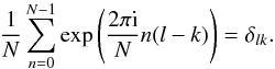
A&A
Volume 556, August 2013
|
|
|---|---|---|
| Article Number | A70 | |
| Number of page(s) | 16 | |
| Section | Cosmology (including clusters of galaxies) | |
| DOI | https://doi.org/10.1051/0004-6361/201321718 | |
| Published online | 30 July 2013 | |
A quasi-Gaussian approximation for the probability distribution of correlation functions ⋆
Argelander-Institut für Astronomie, Universität Bonn,
Auf dem Hügel 71,
53121
Bonn,
Germany
e-mail: This email address is being protected from spambots. You need JavaScript enabled to view it.
; This email address is being protected from spambots. You need JavaScript enabled to view it.
Received:
17
April
2013
Accepted:
1
July
2013
Abstract
Context. Whenever correlation functions are used for inference about cosmological parameters in the context of a Bayesian analysis, the likelihood function of correlation functions needs to be known. Usually, it is approximated as a multivariate Gaussian, though this is not necessarily a good approximation.
Aims. We show how to calculate a better approximation for the probability distribution of correlation functions of one-dimensional random fields, which we call “quasi-Gaussian”.
Methods. Using the exact univariate probability distribution function (PDF) as well as constraints on correlation functions previously derived, we transform the correlation functions to an unconstrained variable for which the Gaussian approximation is well justified. From this Gaussian in the transformed space, we obtain the quasi-Gaussian PDF. The two approximations for the probability distributions are compared to the “true” distribution as obtained from simulations. Additionally, we test how the new approximation performs when used as likelihood in a toy-model Bayesian analysis.
Results. The quasi-Gaussian PDF agrees very well with the PDF obtained from simulations; in particular, it provides a significantly better description than a straightforward copula approach. In a simple toy-model likelihood analysis, it yields noticeably different results than the Gaussian likelihood, indicating its possible impact on cosmological parameter estimation.
Key words: methods: statistical / cosmological parameters / large-scale structure of Universe / galaxies: statistics / cosmology: miscellaneous
Appendices are available in electronic form at http://www.aanda.org
© ESO, 2013
1. Introduction
Correlation functions are an important tool in cosmology, since they constitute one
standard way of using observations to constrain cosmological parameters. The two-point
correlation function ξ(x) obtained from observational data is
usually analyzed in the framework of Bayesian statistics: using Bayes’ theorem  (1)the measured
correlation function ξ is used to quantify how the optimal parameters
θ of the cosmological model change. It is inherent to Bayesian methods
that we need to “plug in” the probability distribution function (PDF) of the data involved.
In the case of correlation functions, this likelihood
ℒ(θ) ≡ p(ξ | θ) is
usually assumed to be a Gaussian. For example in Seljak
& Bertschinger (1993), the authors perform an analysis of the angular
correlation function of the cosmic microwave background (as calculated from COBE data),
stating that a Gaussian is a good approximation for its likelihood, at least near the peak.
Also in common methods of baryon acoustic oscillations (BAO) detection, a Gaussian
distribution of correlation functions is usually assumed (see e.g. Labatie et al. 2012a). While this may be a good approximation in some
cases, there are strong hints that there may in other cases be strong deviations from a
Gaussian likelihood. For example in Hartlap et al.
(2009), using independent component analysis, a significant non-Gaussianity in the
likelihood is detected in the case of a cosmic shear study.
(1)the measured
correlation function ξ is used to quantify how the optimal parameters
θ of the cosmological model change. It is inherent to Bayesian methods
that we need to “plug in” the probability distribution function (PDF) of the data involved.
In the case of correlation functions, this likelihood
ℒ(θ) ≡ p(ξ | θ) is
usually assumed to be a Gaussian. For example in Seljak
& Bertschinger (1993), the authors perform an analysis of the angular
correlation function of the cosmic microwave background (as calculated from COBE data),
stating that a Gaussian is a good approximation for its likelihood, at least near the peak.
Also in common methods of baryon acoustic oscillations (BAO) detection, a Gaussian
distribution of correlation functions is usually assumed (see e.g. Labatie et al. 2012a). While this may be a good approximation in some
cases, there are strong hints that there may in other cases be strong deviations from a
Gaussian likelihood. For example in Hartlap et al.
(2009), using independent component analysis, a significant non-Gaussianity in the
likelihood is detected in the case of a cosmic shear study.
A more fundamental approach to this is performed in Schneider & Hartlap (2009): under very general conditions, it is shown that there exist constraints on the correlation function, meaning that a valid correlation function is confined to a certain range of values. This proves that the likelihood of the correlation function cannot be truly Gaussian: a Gaussian distribution has infinite support, meaning that it is non-zero also in “forbidden” regions.
Thus, it is necessary to look for a better description of the likelihood than a Gaussian. This could lead to a more accurate data analysis and thus, in the end, result in more precise constraints on the cosmological parameters obtained by such an analysis. It is also worth noting that Carron (2013) has shown some inconsistencies of Gaussian likelihoods: for the case of power spectrum estimators, using Gaussian likelihoods can assign too much information to the data and thus violate the Cramér-Rao inequality. Along the same lines, Sun et al. (2013) show that the use of Gaussian likelihoods in power spectra analyses can have significant impact on the bias and uncertainty of estimated parameters.
Of course, non-Gaussian likelihood functions have been studied before: for the case of the cosmic shear power spectrum, Sato et al. (2011) use a Gaussian copula to construct a more accurate likelihood function. The use of a copula requires knowledge of the univariate distribution, for which the authors find a good approximation from numerical simulations.
However, in the case of correlation functions, similar work is sparse in the literature, so up to now, no better general approximation than the Gaussian likelihood has been obtained. Obviously, the most fundamental approach to this is to try and calculate the probability distributions of correlation functions analytically: Keitel & Schneider (2011) used a Fourier mode expansion of a Gaussian random field in order to obtain the characteristic function of p(ξ). From it, they calculate the uni- and bivariate probability distribution of ξ through a Fourier transform. Since this calculation turns out to be very tedious, an analytical computation of higher-variate PDFs is probably not feasible. Still, coupling the exact univariate distributions with a Gaussian copula might yield a multivariate PDF that is a far better approximation than the Gaussian one – we will show, however, that this is not the case.
In the main part of this work, we will therefore try a different approach: using a transformation of variables that involves the aforementioned constraints on correlation functions derived in Schneider & Hartlap (2009), we will derive a way of computing a new, “quasi-Gaussian” likelihood function for the correlation functions of one-dimensional Gaussian random fields.
It is notable that the strategy of transforming a random variable in order to obtain a well-known probability distribution (usually a Gaussian one) suggests a comparison to similar attempts: for example, Box-Cox methods can be used to find an optimal variable transformation to Gaussianity (see e.g. Joachimi et al. 2011). We will argue, however, that a Box-Cox approach does not seem to yield satisfactory results in our case.
This work is structured as follows: in , we briefly summarize previous work and explain how to compute the quasi-Gaussian likelihood for correlation functions, which is then tested thoroughly and compared to numerical simulations in . In , we investigate how the new approximation of the likelihood performs in a Bayesian analysis of simulated data, compared to the usual Gaussian approximation. Our attempts to find a new approximation of the likelihood using a copula or Box-Cox approach are presented in . We conclude with a short summary and outlook in .
2. A new approximation for the likelihood of correlation functions
2.1. Notation
We denote a random field by g(x) and define its Fourier
transform as  (2)In order to perform
numerical simulations involving random fields, it is necessary to discretize the field,
i.e. evaluate it at discrete grid points, and introduce boundary conditions: Limiting the
field to an n-dimensional periodic cube with side length
L in real space is equivalent to choosing a grid in
k-space such that the wave number can only take integer multiples of the
smallest possible wave number
Δk = 2π/L. In
order to simulate a field that spans the whole space Rn, we
can choose L such that no structures at larger scales than
L exist. In this case, the hypercube is representative for the whole
field and we can extend it to Rn by imposing periodic boundary
conditions, i.e. by setting (in one dimension)
g(x + L) = g(x).
After discretization, the integral from Eq. (2) simply becomes a discrete Fourier series, and the field can be written as
(2)In order to perform
numerical simulations involving random fields, it is necessary to discretize the field,
i.e. evaluate it at discrete grid points, and introduce boundary conditions: Limiting the
field to an n-dimensional periodic cube with side length
L in real space is equivalent to choosing a grid in
k-space such that the wave number can only take integer multiples of the
smallest possible wave number
Δk = 2π/L. In
order to simulate a field that spans the whole space Rn, we
can choose L such that no structures at larger scales than
L exist. In this case, the hypercube is representative for the whole
field and we can extend it to Rn by imposing periodic boundary
conditions, i.e. by setting (in one dimension)
g(x + L) = g(x).
After discretization, the integral from Eq. (2) simply becomes a discrete Fourier series, and the field can be written as
 (3)where we defined
the Fourier coefficients
(3)where we defined
the Fourier coefficients  (4)The two-point
correlation function of the field is defined as
ξ(x,y) = ⟨g(x)·g∗(y)⟩;
it is the Fourier transform of the power spectrum:
(4)The two-point
correlation function of the field is defined as
ξ(x,y) = ⟨g(x)·g∗(y)⟩;
it is the Fourier transform of the power spectrum: 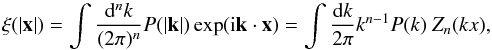 (5)where the function
Zn(η) is obtained from
integrating the exponential over the direction of k. In particular,
Z2(η) = J0(η)
and
Z3(η) = j0(η),
where J0(η) denotes the Bessel function of
the first kind of zero order and j0(η) is the
spherical Bessel function of zero order. In the one-dimensional case, Eq. (5) becomes a simple cosine transform,
(5)where the function
Zn(η) is obtained from
integrating the exponential over the direction of k. In particular,
Z2(η) = J0(η)
and
Z3(η) = j0(η),
where J0(η) denotes the Bessel function of
the first kind of zero order and j0(η) is the
spherical Bessel function of zero order. In the one-dimensional case, Eq. (5) becomes a simple cosine transform,
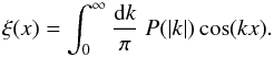 (6)A random field is
called Gaussian if its Fourier components
(6)A random field is
called Gaussian if its Fourier components  are statistically independent and the probability distribution of each
is Gaussian, i.e.
are statistically independent and the probability distribution of each
is Gaussian, i.e. 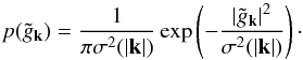 (7)A central property of a
Gaussian random field is that it is entirely specified by its power spectrum, which is
given as a function of σ(| k |):
(7)A central property of a
Gaussian random field is that it is entirely specified by its power spectrum, which is
given as a function of σ(| k |): 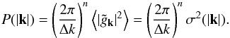 (8)In the following, we
will only be concerned with one-dimensional, periodic Gaussian fields of field length
L, evaluated at N discrete grid points
gi ≡ g(xi),
xi = i L/N.
(8)In the following, we
will only be concerned with one-dimensional, periodic Gaussian fields of field length
L, evaluated at N discrete grid points
gi ≡ g(xi),
xi = i L/N.
2.2. Constraints on correlation functions
As shown in Schneider & Hartlap (2009, hereafter
SH2009), correlation functions cannot take arbitrary values, but are subject to
constraints, originating from the non-negativity of the power spectrum
P(k). The constraints are expressed in terms of the
correlation coefficients  (9)Since we will be
using a gridded approach, we shall denote
ξ(n Δx) ≡ ξn,
where Δx = L/N
denotes the separation between adjacent grid points. The constraints can be written in the
form
(9)Since we will be
using a gridded approach, we shall denote
ξ(n Δx) ≡ ξn,
where Δx = L/N
denotes the separation between adjacent grid points. The constraints can be written in the
form  (10)where the upper and lower
boundaries are functions of the ri with
i < n. SH2009 use two
approaches to calculate the constraints: The first one applies the Cauchy-Schwartz
inequality and yields the following constraints:
(10)where the upper and lower
boundaries are functions of the ri with
i < n. SH2009 use two
approaches to calculate the constraints: The first one applies the Cauchy-Schwartz
inequality and yields the following constraints: 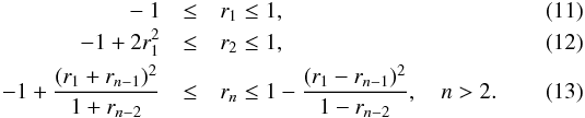 The
second approach involves the covariance matrix C, which for a
one-dimensional random field gi of
N grid points, reads
The
second approach involves the covariance matrix C, which for a
one-dimensional random field gi of
N grid points, reads
 (14)Calculating the
eigenvalues of C and making use of the fact that they have to be
non-negative due to the positive semi-definiteness of C allows the
calculation of constraints on ri for
arbitrary n. As it turns out, for n ≥ 4, the constraints
obtained by this method are different (that is, stricter) than the ones from the
Cauchy-Schwarz inequality – e.g. for n = 4, while the upper bound remains
unchanged compared to Eq. (13), the lower
bound then reads
(14)Calculating the
eigenvalues of C and making use of the fact that they have to be
non-negative due to the positive semi-definiteness of C allows the
calculation of constraints on ri for
arbitrary n. As it turns out, for n ≥ 4, the constraints
obtained by this method are different (that is, stricter) than the ones from the
Cauchy-Schwarz inequality – e.g. for n = 4, while the upper bound remains
unchanged compared to Eq. (13), the lower
bound then reads  (15)Moreover, SH2009 show
that the constraints are “optimal” (in the sense that no stricter bounds can be found for
a general power spectrum) for the one-dimensional case. In more than one dimension,
although the constraints derived by SH2009 still hold, stricter constraints will hold due
to the multidimensional integration in Eq. (5) and the isotropy of the field.
(15)Moreover, SH2009 show
that the constraints are “optimal” (in the sense that no stricter bounds can be found for
a general power spectrum) for the one-dimensional case. In more than one dimension,
although the constraints derived by SH2009 still hold, stricter constraints will hold due
to the multidimensional integration in Eq. (5) and the isotropy of the field.
One can show that the constraints are obeyed by generating realizations of the correlation function of a Gaussian random field with a power spectrum that is randomly drawn for each realization (we will elaborate more on these simulations in ).
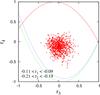 |
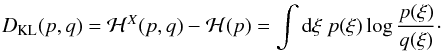
Fig. 1 Constraints in the r3-r4-plane (i.e. with fixed r1 and r2) for a field with N = 16 grid points and randomly drawn power spectra. For the lower bound, the results from the Cauchy-Schwarz inequality (green) as well as from the covariance matrix approach (blue) are shown. |
In addition to the plots shown in SH2009, we show the r3-r4-plane for illustration, see . Note that the admissible region is populated only sparsely, since the constraints on r3 depend explicitly on r1 and r2, so we have to fix those, resulting in only 845 of the simulated 400 000 realizations that have r1 and r2 close to the fixed values. Figure 1 shows the lower bounds r4l as calculated from the Cauchy-Schwarz inequality and from the covariance matrix method. One can see that the latter (plotted in blue) is slightly stricter than the former, shown in green.
A central idea of SH2009 on the way to a better approximation for the PDF of correlation
functions is to transform the correlation function to a space where no constraints exist,
and where the Gaussian approximation is thus better justified. This can be done by
defining  (16)The transformation to
xn maps the allowed range of
rn to the interval
(16)The transformation to
xn maps the allowed range of
rn to the interval
 , which
is then mapped onto the entire real axis
, which
is then mapped onto the entire real axis  by the
inverse hyperbolic tangent. The choice of atanh by SH2009 was an “educated guess”, rather
than based on theoretical arguments.
by the
inverse hyperbolic tangent. The choice of atanh by SH2009 was an “educated guess”, rather
than based on theoretical arguments.
2.3. Simulations
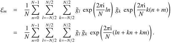
In the following, we will explain the simulations we use to generate realizations of the correlation function of a Gaussian random field with a given power spectrum. A usual method to do this is the following: one can draw realizations of the field in Fourier space, i.e. according to Eq. (7), where the width of the Gaussian is given by the theoretical power spectrum via Eq. (8). The field is then transformed to real space, and ξ can then be calculated using an estimator based on the gi.
We developed an alternative method: Since we are not interested in the field itself, we
can save memory and CPU time by directly drawing realizations of the power spectrum. To do
so, we obviously need the probability distribution of the power spectrum components
Pi ≡ P(ki) ≡ P(i Δk)
– this can be calculated easily from Eq. (7), since for one realization,  . The calculation
yields
. The calculation
yields  (17)where
H(ξ) denotes the Heaviside step function. Thus, for
Gaussian random fields, each power spectrum mode follows an exponential distribution with
a width given by the model power
(17)where
H(ξ) denotes the Heaviside step function. Thus, for
Gaussian random fields, each power spectrum mode follows an exponential distribution with
a width given by the model power  .
.
For each realization of the power spectrum, the correlation function can then be computed
using a discrete cosine transform given by a discretization of Eq. (6),  (18)This method can in
principle be generalized to higher-dimensional fields, where the savings in memory and CPU
usage will of course be far greater. It is clear that this new method should yield the
same results as the established one (which involves generating the field). We confirmed
this fact numerically; additionally, we give a proof for the equivalence of the two
methods in Appendix A.
(18)This method can in
principle be generalized to higher-dimensional fields, where the savings in memory and CPU
usage will of course be far greater. It is clear that this new method should yield the
same results as the established one (which involves generating the field). We confirmed
this fact numerically; additionally, we give a proof for the equivalence of the two
methods in Appendix A.
In order to draw the power spectrum components
Pi according to the PDF given in Eq. (17), we integrate and invert this equation,
yielding 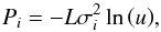 (19)where
u is a uniformly distributed random number with
u ∈ [0,1] (see Press et al. 2007 for a more elaborate explanation on random deviates).
(19)where
u is a uniformly distributed random number with
u ∈ [0,1] (see Press et al. 2007 for a more elaborate explanation on random deviates).
As an additional improvement to our simulations, we implement a concept called quasi-random (or “sub-random”) sampling; again, see Press et al. (2007) for more details: Instead of drawing uniform deviates u for each component Pi, we use quasi-random points, thus ensuring that we sample the whole hypercube of power spectra as fully as possible, independent of the sample size. One way to generate quasi-randomness is by using a so-called Sobol’ sequence, see e.g. Joe & Kuo (2008) for explanations. Implementations for Sobol’ sequences exist in the literature, we use a C++ program available at the authors’ website http://web.maths.unsw.edu.au/~fkuo/sobol/.
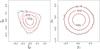 |
Fig. 2 Iso-probability contours of p(ξ3,ξ6) (left) and p(y3,y6) (right) for 400 000 realizations of a field with N = 32 grid points and a Gaussian power spectrum with Lk0 = 80. The dashed red contours show the best-fitting Gaussian approximations in both cases. |
To illustrate the non-Gaussian probability distribution of correlation functions, the left-hand part of shows the iso-probability contours of p(ξ3,ξ6), i.e. the PDF of the correlation function for a lag equal to 3 and 6 times the distance between adjacent grid points, calculated over the 400 000 realizations of a field with N = 32 grid points. For the shape of the power spectrum, we choose a Gaussian, i.e. σ2(k) ∝ exp(−(k/k0)2), whose width k0 is related to the field length L by Lk0 = 80. For simplicity, we will refer to this as a “Gaussian power spectrum” in the following, indicating its shape P(k). The chosen Gaussian shape of the power spectrum should not be confused with the Gaussianity of the random field. The red contours show the corresponding Gaussian with the same mean and standard deviation. It is clearly seen that the Gaussian approximation is not particularly good. In order to check whether the Gaussian approximation is justified better in the new variables yi, we transform the simulated realizations of the correlation function to y-space, using the constraints riu and ril from the covariance matrix approach, which we calculate exploiting the matrix methods explained in SH2009. The right-hand part of shows the probability distribution p(y3,y6) and the Gaussian with mean and covariance as computed from { y3,y6 }. Obviously, the transformed variables follow a Gaussian distribution much more closely than the original correlation coefficients.
2.4. Transformation of the PDF
Before actually assessing how good the Gaussian approximation in y-space is, we will first try to make use of it and develop a method to obtain a better approximation of the probability distributions in r- and, in the end, ξ-space.
Assuming a Gaussian distribution in y-space, we can calculate the PDF in
r-space as  (20)Here,
Jr → y denotes the
Jacobian matrix of the transformation defined in Eq. (16), so
(20)Here,
Jr → y denotes the
Jacobian matrix of the transformation defined in Eq. (16), so ![Mathematical equation: \begin{eqnarray} \label{eq:jacobian} J_{ij}^{r\rightarrow y}&=& \frac{\partial y_i}{\partial r_j}=\frac{\partial y_i}{\partial x_i}\frac{\partial x_i}{\partial r_j} =\frac{1}{1-x_i^2}\frac{\partial x_i}{\partial r_j}\nonumber\\[1mm] &=& \frac{2}{\Deltai^2-(2r_i-\riu-\ril)^2}\nonumber\\[3mm] &&\times \left[\Deltai\delta_{ij}-(r_i-\ril)\frac{\partial\riu}{\partial r_j}-(\riu-r_i)\frac{\partial\ril}{\partial r_j}\right]\cdot \end{eqnarray}](/articles/aa/full_html/2013/08/aa21718-13/aa21718-13-eq83.png) (21)Since
the lower and upper bounds ril and
riu only depend on the
rj with
j < i, all partial derivatives
with i ≤ j vanish. Thus,
Jr → y is a lower
triangular matrix, and its determinant can simply be calculated as the product of its
diagonal entries. Hence, the partial derivatives
∂ril/∂rj
and
∂riu/∂rj
of the bounds are not needed.
(21)Since
the lower and upper bounds ril and
riu only depend on the
rj with
j < i, all partial derivatives
with i ≤ j vanish. Thus,
Jr → y is a lower
triangular matrix, and its determinant can simply be calculated as the product of its
diagonal entries. Hence, the partial derivatives
∂ril/∂rj
and
∂riu/∂rj
of the bounds are not needed.
As an example, we calculate the bivariate distribution p(r1,r2), assuming p(y1,y2) to be a Gaussian with mean and covariance matrix obtained from the 400 000 simulated realizations. Figure 3 shows p(r1,r2) from the simulations (solid contours) as well as the transformed Gaussian (dashed red contours) – obviously, it is a far better approximation of the true distribution than a Gaussian in r-space. The upper and lower bounds on r2 are also shown.
In the next step, we will show how to compute the quasi-Gaussian likelihood for the
correlation function ξ, since ξ (and not
r) is the quantity that is actually measured in reality. The
determinant of the Jacobian for the transformation ξ → r
is simple, since
ri = ξi/ξ0;
however, we have to take into account that in ξ-space, an additional
variable, namely ξ0, exists. Thus, we have to write down the
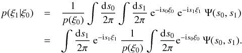
transformation as follows: 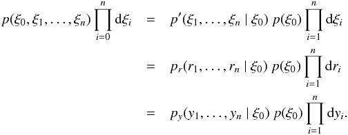 (22)We
see that the n-variate PDF in ξ-space explicitly depends
on the distribution of the correlation function at zero lag,
p(ξ0). In the following, we will use the
analytical formula derived in Keitel & Schneider
(2011). In the univariate case, it reads
(22)We
see that the n-variate PDF in ξ-space explicitly depends
on the distribution of the correlation function at zero lag,
p(ξ0). In the following, we will use the
analytical formula derived in Keitel & Schneider
(2011). In the univariate case, it reads 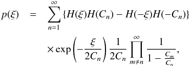 (23)where
H(ξ) again denotes the Heaviside step function and the
Cn are given by
(23)where
H(ξ) again denotes the Heaviside step function and the
Cn are given by
 . Here, x is
the lag parameter, and thus, for the zero-lag correlation function
ξ0,
. Here, x is
the lag parameter, and thus, for the zero-lag correlation function
ξ0,  holds. When
evaluating Eq. (23), we obviously have to
truncate the summation at some N′. Since this number of modes
N′ corresponds to the number of grid points in Fourier space
(which is half the number of real-space grid points N, but as explained
in Appendix A, we set the highest mode to zero), we
truncate at N′ = N/2−1.
As shows, the PDF of the { ξ0 }-sample (black dots) agrees
perfectly with the result from the analytical formula (red curve).
holds. When
evaluating Eq. (23), we obviously have to
truncate the summation at some N′. Since this number of modes
N′ corresponds to the number of grid points in Fourier space
(which is half the number of real-space grid points N, but as explained
in Appendix A, we set the highest mode to zero), we
truncate at N′ = N/2−1.
As shows, the PDF of the { ξ0 }-sample (black dots) agrees
perfectly with the result from the analytical formula (red curve).
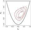 |
Fig. 3 p(r1,r2) for a field with N = 32 grid points and a Gaussian power spectrum with Lk0 = 80. The dashed red contours show the transformed Gaussian approximation from y-space. |
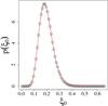 |
Fig. 4 p(ξ0) for a random field with N = 32 grid points and a Gaussian power spectrum with Lk0 = 80: the black dots show the PDF from the simulation, whereas the red curve was calculated from the analytical formula, using N/2−1 = 15 modes and the same field length and power spectrum. |
As an illustrative example, we will show how to compute the quasi-Gaussian approximation of p(ξ1,ξ2). In order to do so, we need to calculate the conditional probability p(ξ1,ξ2 | ξ0) and then integrate over ξ0. To perform the integration, we divide the ξ0-range obtained from the simulations into bins and transform the integral into a discrete sum.
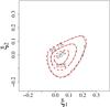 |
Fig. 5 p(ξ1,ξ2) for a field with N = 32 grid points and a Gaussian power spectrum with Lk0 = 80. The dashed red contours show the transformed Gaussian approximation from y-space. |
Furthermore, we have to incorporate a potential ξ0-dependence of the covariance matrix and mean of y. We examine this dependence in – clearly, the covariance matrix shows hardly any ξ0-dependence, so as a first try, we treat it as independent of ξ0 and simply use the covariance matrix obtained from the full sample. In contrast, the mean does show a non-negligible ξ0-dependence, as the top panels of illustrate. However, this dependence seems to be almost linear, with a slope that decreases for higher lag parameter. Thus, since the calculation of the multivariate quasi-Gaussian PDF involves computing a conditional probability with a fixed ξ0-value as an intermediate step, we can easily handle the ξ0-dependence by calculating the mean only over realizations close to the current value of ξ0 – in the exemplary calculation of p(ξ1,ξ2) discussed here, we average only over those realizations with a ξ0-value in the current bin of the ξ0-integration.
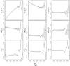 |
Fig. 6 Mean (top row) and standard deviation (second row) of yn for different n as well as different off-diagonal elements of the covariance matrix C(⟨ yn ⟩) (third row) as functions of ξ0, determined from simulations; the error bars show the corresponding standard errors (which depend on the number of realizations with a value of ξ0 that lies in the current bin). |
Our final result for p(ξ1,ξ2) is shown in . Clearly, the quasi-Gaussian approximation (red dashed contours) follows the PDF obtained from the simulations quite closely. Note that the quasi-Gaussian PDF was calculated using only 10 ξ0-bins for the integration, which seems sufficient to obtain a convergent result.
It should be noted that, although our phenomenological treatment of the ξ0-dependence of mean and covariance matrix seems to be sufficiently accurate to give satisfying results, the analytical calculation of this dependence would of course be preferable, since it could improve the accuracy and the mathematical consistency of our method. We show this calculation in Appendix B. However, since the results turn out to be computationally impractical and also require approximations, thus preventing a gain in accuracy, we refrain from using the analytical mean and covariance matrix.
3. Quality of the quasi-Gaussian approximation
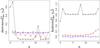 |
Fig. 7 Skewness (left-hand panel) and kurtosis (right-hand panel) of { ξn } (black circles) and { yn } (red triangles) as functions of lag n, for a Gaussian power spectrum with Lk0 = 80. The blue squares show the skewness/kurtosis of Gaussian samples of the same length, mean and variance as the corresponding samples { yn }. |
For the bivariate distributions we presented so far, it is apparent at first glance that the quasi-Gaussian likelihood provides a more accurate approximation than the Gaussian one. However, we have not yet quantified how much better it actually is.
There are, in principle, two ways to address this: for one, we can directly test the Gaussian approximation in y-space. We will do so in , making use of the fact that the moments of a Gaussian distribution are well-known. Alternatively, we can perform tests in ξ-space, which we will do in . Although in this case, we have to resort to more cumbersome methods, this approach is actually better, since it allows for a direct comparison to the Gaussian approximation in ξ-space. Furthermore, it is more significant, because it incorporates testing the transformation, especially our treatment of the ξ0-dependence of the mean and covariance in y-space.
3.1. Tests in y-space
In order to test the quality of the Gaussian approximation in y-space,
we calculate moments of the univariate distributions
p(yn), as obtained from
our numerical simulations. The quantities we are interested in are the (renormalized)
third-order moment, i.e. the skewness 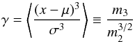 (24)as
well as kurtosis κ, which is essentially the fourth-order moment:
(24)as
well as kurtosis κ, which is essentially the fourth-order moment:
 (25)Here,
mi = ⟨ (x − μ)i ⟩
denote the central moments. Defined like this, both quantities are zero for a Gaussian
distribution.
(25)Here,
mi = ⟨ (x − μ)i ⟩
denote the central moments. Defined like this, both quantities are zero for a Gaussian
distribution.
The results can be seen in : the red triangles show the skewness/kurtosis of the 400 000 simulated { yn }-samples (again for a field with N = 32 grid points and a Gaussian power spectrum with Lk0 = 80). Clearly, both moments deviate from zero, which cannot be explained solely by statistical scatter: the blue squares show the skewness/kurtosis of Gaussian samples of the same length, mean and variance as the corresponding samples { yn }, and they are quite close to zero. However, it can also be clearly seen that the skewness and kurtosis of the univariate distributions in ξ-space (shown as black circles) deviate significantly more from zero, showing that the Gaussian approximation of the univariate distributions is far more accurate in y- than in ξ-space – this is true also for other lag parameters than the ones used in the examples of the previous sections.
Note that although we used N = 32 (real-space) grid points for our simulations, we only show the moments up to n = 15, since the ξn with higher n contain no additional information due to the periodic boundary conditions (and thus, the corresponding yn have no physical meaning). Additionally, by construction, the y0-component does not exist.
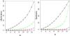 |
Fig. 8 Mardia’s skewness (left-hand panel) and kurtosis (right-hand panel) of n-variate { ξ }- (black circles) and { y }-samples (red, upward triangles) for a Gaussian power spectrum with Lk0 = 80. The green, downward triangles show the skewness/kurtosis of { y }-samples obtained under the assumption of a Gaussian { ξ }-sample, and the blue squares show the skewness/kurtosis of Gaussian samples. See text for more details. |
Since the fact that the univariate PDFs
p(yi) are “quite
Gaussian” does not imply that the full multivariate distribution
p(y) is well described by a multivariate Gaussian
distribution, we also perform a multivariate test. While numerous tests for multivariate
Gaussianity exist (see e.g. Henze 2002, for a
review), we confine our analysis to moment-based tests. To do so, it is necessary to
generalize skewness and kurtosis to higher dimensions – we use the well-established
definitions by Mardia (1970, 1974): considering a sample of d-dimensional vectors
xi, a measure of skewness for a
d-variate distribution can be written as
 (26)where
n denotes the sample size, and μ and
C are the mean and covariance matrix of the sample. The corresponding
kurtosis measure is
(26)where
n denotes the sample size, and μ and
C are the mean and covariance matrix of the sample. The corresponding
kurtosis measure is  (27)where we subtracted the
last term to make sure that the kurtosis of a Gaussian sample is zero.
(27)where we subtracted the
last term to make sure that the kurtosis of a Gaussian sample is zero.
Figure 8 shows the results of the multivariate test. For the same simulation run as before (using only 5000 realizations to speed up calculations), the skewness and kurtosis of the n-variate distributions, i.e. p(ξ0,...,ξn − 1) (black circles) and p(y1,...,yn) (red, upward triangles) are plotted as a function of n. For comparison, the blue squares show the moments of the n-variate distributions marginalized from a 15-variate Gaussian. It is apparent that also in the multivariate case, the assumption of Gaussianity is by far better justified for the transformed variables y than for ξ, although the approximation is not perfect.
To avert comparing PDFs of different random variables (namely ξ and y), we perform an additional check: we draw a 15-variate Gaussian sample in ξ-space and transform it to y-space (using only the realizations which lie inside the constraints); the corresponding values of skewness and kurtosis are shown as green, downward triangles. Clearly, they are by far higher than those obtained for the “actual” y-samples, further justifying our approach.
3.2. Tests in ξ-space
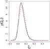 |
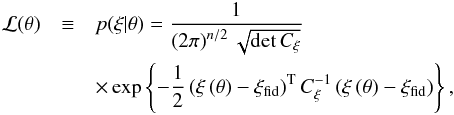
Fig. 9 p(ξ1) for a field with N = 32 grid points and a Gaussian power spectrum with Lk0 = 80. The black curve is from simulations, the blue dot-dashed curve shows the best-fitting Gaussian, and the other two curves show the quasi-Gaussian approximation using a constant covariance matrix (green dotted curve) and incorporating its ξ0-dependence (red dashed curve). |
In the following, we will directly compare the “true” distribution of the correlation functions as obtained from simulations to the Gaussian and the quasi-Gaussian PDF. As an example, we consider the univariate PDF p(ξ1). Figure 9 shows the different distributions – it is clear by eye that the quasi-Gaussian PDF is a far better approximation for the true (black) distribution than the best-fitting Gaussian (shown in blue and dot-dashed). In addition, it becomes clear that we can improve our results by incorporating the ξ0-dependence of the covariance matrix: while the assumption of a constant covariance matrix already yields a quasi-Gaussian (shown as the green dotted curve) which is close to the true distribution, the red dashed curve representing the quasi-Gaussian which incorporates the ξ0-dependence of the covariance matrix (in the same way as was done for the mean) is practically indistinguishable from the true PDF. In the following, we would like to quantify this result.
While a large variety of rigorous methods for comparing probability distributions exist,
we will at first present an intuitive test: a straightforward way of quantifying how
different two probability distributions p(ξ) and
q(ξ) are is to integrate over the absolute value of
their difference, defining the “integrated difference”  (28)Here, we take
p to be the “true” PDF as obtained from the simulations, and
q the approximation. In order to calculate them, we introduce binning,
meaning that we again split the range of ξ1 in bins of width
Δξ and discretize Eq. (28). The values we obtain show a slight dependence on the number of bins – the
reason is Poisson noise, since Δint is not exactly zero even if the
approximation is perfect, i.e. if the sample with the empirical PDF p was
indeed drawn from the distribution q. The dependence on the binning
becomes more pronounced in the multivariate case, but in the univariate example we
consider here, Δint provides a coherent way of comparing the distributions.
Namely, if we divide the range of ξ1 into 100 bins (the same
number we used for ), we obtain Δint ≈ 0.18 for the Gaussian PDF and
Δint ≈ 0.025 (0.011) for the quasi-Gaussian PDF with constant
(ξ0-dependent) covariance matrix, thus yielding a difference
of more than one order of magnitude in the latter case.
(28)Here, we take
p to be the “true” PDF as obtained from the simulations, and
q the approximation. In order to calculate them, we introduce binning,
meaning that we again split the range of ξ1 in bins of width
Δξ and discretize Eq. (28). The values we obtain show a slight dependence on the number of bins – the
reason is Poisson noise, since Δint is not exactly zero even if the
approximation is perfect, i.e. if the sample with the empirical PDF p was
indeed drawn from the distribution q. The dependence on the binning
becomes more pronounced in the multivariate case, but in the univariate example we
consider here, Δint provides a coherent way of comparing the distributions.
Namely, if we divide the range of ξ1 into 100 bins (the same
number we used for ), we obtain Δint ≈ 0.18 for the Gaussian PDF and
Δint ≈ 0.025 (0.011) for the quasi-Gaussian PDF with constant
(ξ0-dependent) covariance matrix, thus yielding a difference
of more than one order of magnitude in the latter case.
A well-established measure for the “distance” between two probability distributions
p and q is the Kullback-Leibler (K-L) divergence,
which is defined as the difference of the cross-entropy ℋX of
p and q and the entropy ℋ of p:
 (29)As
before, the values obtained vary slightly with the number of bins. Using 100
ξ1-bins yields DKL ≈ 0.04 for
the Gaussian and DKL ≈ 0.001 for the quasi-Gaussian PDF with a
constant covariance matrix. Here, incorporating the
ξ0-dependence of the covariance matrix has an even stronger
impact, resulting in DKL ≈ 0.0002. Hence, the K-L divergence
gives us an even stronger argument for the increased accuracy of the quasi-Gaussian
approximation compared to the Gaussian case.
(29)As
before, the values obtained vary slightly with the number of bins. Using 100
ξ1-bins yields DKL ≈ 0.04 for
the Gaussian and DKL ≈ 0.001 for the quasi-Gaussian PDF with a
constant covariance matrix. Here, incorporating the
ξ0-dependence of the covariance matrix has an even stronger
impact, resulting in DKL ≈ 0.0002. Hence, the K-L divergence
gives us an even stronger argument for the increased accuracy of the quasi-Gaussian
approximation compared to the Gaussian case.
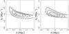 |
Fig. 10 Posterior probability for the power spectrum parameters
|


4. Impact of the quasi-Gaussian likelihood on parameter estimation
In this section, we will check which impact the new, quasi-Gaussian approximation of the likelihood has on the results of a Bayesian parameter estimation analysis. As data, we generate 400 000 realizations of the correlation function of a Gaussian random field with N = 64 grid points and a Gaussian power spectrum with L k0 = 100. From this data, we wish to obtain inference about the parameters of the power spectrum (i.e. its amplitude A and its width k0) according to Eq. (1), so θ = (A,k0). To facilitate this choice of parameters, we parametrize the power spectrum as P(k) = A·100/(Lk0) exp { −(k/k0)2 }, where we choose A = 1 Mpc and k0 = 1 Mpc-1 as fiducial values (corresponding to L k0 = 100 and a field length L = 100 Mpc). Since we use a flat prior for θ and the denominator (the Bayesian evidence) acts solely as a normalization in the context of parameter estimation, the shape of the posterior p(θ | ξ) is determined entirely by the likelihood.
For the likelihood, we first use the Gaussian approximation
 (30)where
ξ ≡ (ξ0,...,ξn − 1)T
and Cξ denotes the covariance matrix computed
from the { ξ }-sample; note that we use only n = 32
ξ-components, since the last 32 components yield no additional
information due to periodicity. In an analysis of actual data, the measured value of the
correlation function would have to be inserted as mean of the Gaussian distribution – since
in our toy-model analysis, we use our simulated sample of correlation functions as data, we
insert
(30)where
ξ ≡ (ξ0,...,ξn − 1)T
and Cξ denotes the covariance matrix computed
from the { ξ }-sample; note that we use only n = 32
ξ-components, since the last 32 components yield no additional
information due to periodicity. In an analysis of actual data, the measured value of the
correlation function would have to be inserted as mean of the Gaussian distribution – since
in our toy-model analysis, we use our simulated sample of correlation functions as data, we
insert  instead,
which is practically identical to the sample mean of the generated realizations.
instead,
which is practically identical to the sample mean of the generated realizations.
For a second analysis, we transform the simulated realizations of the correlation function
to y-space and adopt the quasi-Gaussian approximation, meaning that we
calculate the likelihood as described in : ![Mathematical equation: \begin{eqnarray} \label{eq:qg_likelihood} p(\xi|\vec{\theta}) &=& \frac{1}{\left(2\pi\right)^{(n-1)/2} \sqrt{\det C_y}} \nonumber\\[1mm] &&\times \exp\left\lbrace -\frac{1}{2} \transpose{\left(\vec y\left(\vec\theta\right)-\left\langle\vec y\left(\xi_0\right)\right\rangle\right)} \cdot C^{-1}_y\cdot \left(\vec y\left(\vec\theta\right)-\left\langle\vec y\left(\xi_0\right)\right\rangle\right) \right\rbrace \nonumber\\[1mm] &&\times p(\xi_0) \cdot \left|\det\left(J^{\xi\rightarrow y}\right)\right|. \end{eqnarray}](/articles/aa/full_html/2013/08/aa21718-13/aa21718-13-eq167.png) (31)Here,
instead of inserting the fiducial value yfid as “measured value”, we
incorporate the ξ0-dependence of the mean ⟨ y ⟩ in
the same way as previously described, meaning by calculating the average only over those
realizations with a ξ0-value close to the “current” value of
ξ0, which is the one determined by the fixed value of
θ, i.e. ξ0(θ). In contrast
to that, Cy denotes the covariance matrix of
the full y-sample, meaning that we neglect its
ξ0-dependence, although we have shown in that incorporating
this dependence increases the accuracy of the quasi-Gaussian approximation. The reason for
this is that for some values of ξ0, the number of realizations
with a ξ0-value close to it is so small that the sample
covariance matrix becomes singular. However, since the toy-model analysis presented in this
section is about a proof of concept rather than about maximizing the accuracy, this is a
minor caveat – of course, when applying our method in an analysis of real data, the
ξ0-dependence of
Cy should be taken into account. It should
also be mentioned that apart from the ξ0-dependence, we also
neglect any possible dependence of the covariance matrix on the model parameters
θ, since this is not expected to have a strong influence on parameter
estimation (for example in the case of BAO studies, Labatie
et al. 2012b show that even if C does have a slight dependence on
the model parameters, incorporating it in a Bayesian analysis only has a marginal effect on
cosmological parameter constraints).
(31)Here,
instead of inserting the fiducial value yfid as “measured value”, we
incorporate the ξ0-dependence of the mean ⟨ y ⟩ in
the same way as previously described, meaning by calculating the average only over those
realizations with a ξ0-value close to the “current” value of
ξ0, which is the one determined by the fixed value of
θ, i.e. ξ0(θ). In contrast
to that, Cy denotes the covariance matrix of
the full y-sample, meaning that we neglect its
ξ0-dependence, although we have shown in that incorporating
this dependence increases the accuracy of the quasi-Gaussian approximation. The reason for
this is that for some values of ξ0, the number of realizations
with a ξ0-value close to it is so small that the sample
covariance matrix becomes singular. However, since the toy-model analysis presented in this
section is about a proof of concept rather than about maximizing the accuracy, this is a
minor caveat – of course, when applying our method in an analysis of real data, the
ξ0-dependence of
Cy should be taken into account. It should
also be mentioned that apart from the ξ0-dependence, we also
neglect any possible dependence of the covariance matrix on the model parameters
θ, since this is not expected to have a strong influence on parameter
estimation (for example in the case of BAO studies, Labatie
et al. 2012b show that even if C does have a slight dependence on
the model parameters, incorporating it in a Bayesian analysis only has a marginal effect on
cosmological parameter constraints).
The θ-dependence of the last two terms also merits some discussion, in
particular, the role of the fiducial model parameters θfid has
to be specified: while the Gaussian likelihood discussed previously is of course centered
around the fiducial values by construction, since  is inserted
as mean of the Gaussian distribution, this cannot be done in the case of the quasi-Gaussian
likelihood due to its more complicated mathematical form.
is inserted
as mean of the Gaussian distribution, this cannot be done in the case of the quasi-Gaussian
likelihood due to its more complicated mathematical form.
The p(ξ0)-term in Eq. (31) can be treated in a straightforward way: namely, we fix the shape of the PDF p(ξ0) by determining it from the fiducial power spectrum parameters θfid and then evaluate it at the current value ξ0(θ). Thus, we compute this term as pθfid(ξ0(θ)) – in other words, we use θfid to fix Cn as well as Cm and then evaluate Eq. (23) at ξ0(θ).
The last term, i.e. the determinant of the transformation matrix, however, has to be evaluated for the fiducial value, yielding | det(Jξ → y(θfid)) |. Thus, this term has no θ-dependence at all and plays no role in parameter estimation; similarly to the Bayesian evidence, it does not have to be computed, but can rather be understood as part of the normalization of the posterior. This can be explained in a more pragmatic way: assume that a specific value of ξ has been measured and one wants to use it for inference on the underlying power spectrum parameters, incorporating the quasi-Gaussian likelihood. Then one would transform the measurement to y-space and rather use the resulting y-vector as data in the Bayesian analysis than ξ, and thus, the | detJ |-term would not even show up when writing down the likelihood. Here, we nonetheless included it in order to follow the train of thought from and for better comparison with the Gaussian likelihood in ξ-space.
Note that the previous argument cannot be applied to the p(ξ0)-term: calculating it as p(ξ0(θfid) | θfid) (i.e. as independent of θ, making it redundant for parameter estimation), would yield biased results for two reasons: first, the transformation from ξ to y involves only ratios ξi/ξ0, which means that one would neglect large parts of the information contained in ξ0 – in the case discussed here, this would lead to a large degeneracy in the amplitude A of the power spectrum. Furthermore, incorporating the non-negligible ξ0-dependence of the mean ⟨ y ⟩ immediately requires the introduction of the conditional probability in Eq. (22), thus automatically introducing the p(ξ0)-term.
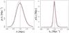 |
Fig. 11 Marginalized posterior probabilities for the power spectrum parameters A and k0. The solid black curves are the results obtained from the Gaussian likelihood, whereas the red dot-dashed curves show the results from the quasi-Gaussian analysis. |
The resulting posteriors can be seen in , where the left-hand panel shows the result for the case of a Gaussian likelihood, and the right-hand one is the result of the quasi-Gaussian analysis. Already for this simple toy model, the impact of the more accurate likelihood on the posterior is visible. The difference may be larger for a different choice of power spectrum, where the deviation of the likelihood from a Gaussian is more pronounced. Nonetheless, it is evident that the change in the shape of the contours is noticeable enough to have an impact on cosmological parameter estimation.
Figure 11 shows the marginalized posteriors for A and k0, again for the Gaussian (black solid curve) and the quasi-Gaussian (red dot-dashed curve) case. As for the full posterior, there is a notable difference. While it may seem alarming that the marginalized posteriors in the quasi-Gaussian case are not centered around the fiducial value, this is in fact not worrisome: first, as a general remark about Bayesian statistics, it is important to keep in mind that there are different ways of obtaining parameter estimates, and in the case of a skewed posterior (as the quasi-Gaussian one), the “maximum a posteriori” (MAP) is not necessarily the most reasonable one. Furthermore, in our case, it should again be stressed that the Gaussian likelihood is of course constructed to be centered around the fiducial value, since θfid is explicitly put in as mean of the distribution, whereas the quasi-Gaussian likelihood is mainly constructed to obey the boundaries of the correlation functions. These are mathematically fundamental constraints, and thus, although none of the two methods are guaranteed to be bias-free, the quasi-Gaussian one should be favored.
5. Alternative approaches
In this section, we briefly investigate two potential alternative ways of finding a new approximation for the likelihood of correlation functions, namely a copula approach and a method involving Box-Cox transformations.
5.1. A copula approach
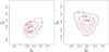 |
Fig. 12 p(ξ1,ξ2) (left) and p(ξ3,ξ6) (right) for a field with N = 32 grid points and a Gaussian power spectrum with Lk0 = 80. The dashed red contours show the approximation obtained from a Gaussian copula. |
Since the exact univariate PDF of ξ is known (Keitel & Schneider 2011), using a copula approach to compute the
correlation function likelihood seems to be an obvious step. According to the definition
of the copula, the joint PDF of n random variables
ξi can be calculated from the univariate
distributions
pi(ξi)
as 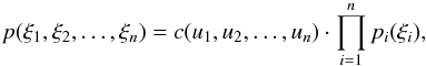 (32)where the copula
density function c depends on
ui = Pi(ξi),
i.e. on the cumulative distribution functions (CDFs) of
ξi. In the simplest case, the copula
function is assumed to be a Gaussian.
(32)where the copula
density function c depends on
ui = Pi(ξi),
i.e. on the cumulative distribution functions (CDFs) of
ξi. In the simplest case, the copula
function is assumed to be a Gaussian.
Copulae have previously been used in cosmology, e.g. for the PDF of the density field of
large-scale structure (Scherrer et al. 2010), or
the weak lensing convergence power spectrum (see Sato et
al. 2011 and its companion paper Sato et al.
2010). In the case of a Gaussian copula, the bivariate joint PDF can be
calculated (see e.g. Sato et al. 2011) as
![Mathematical equation: \begin{eqnarray} \label{eq:copula_xi_bivariate} p\left(\xi_1,\xi_2\right) &=& \frac{1}{\sqrt{2\pi\ \det\left(C\right)}}\ \exp\left\lbrace -\frac{1}{2}\transpose{\left(\vec q -\vec \mu\right)} C^{-1} \left(\vec q -\vec \mu\right)\right\rbrace\nonumber\\[3mm] &&\times \prod_{i=1}^2\left(\frac{1}{\sqrt{2\pi}\sigma_i}\ \exp\left\lbrace -\frac{\left(q_i-\mu_i\right)^2}{2\sigma_i^2}\right\rbrace \right)^{-1} p\left(\xi_i\right), \end{eqnarray}](/articles/aa/full_html/2013/08/aa21718-13/aa21718-13-eq187.png) (33)where
(33)where
 .
Here, μ and C denote the mean and covariance matrix of
the copula function, Φμ,σ is the Gaussian CDF. Note that
contrary to our usual notation, here the indices of ξ are purely a
numbering, and Eq. (33) can in fact be
applied for arbitrary lags.
.
Here, μ and C denote the mean and covariance matrix of
the copula function, Φμ,σ is the Gaussian CDF. Note that
contrary to our usual notation, here the indices of ξ are purely a
numbering, and Eq. (33) can in fact be
applied for arbitrary lags.
To calculate the copula likelihood, we implement the analytical univariate formulae for pi(ξi) and Pi(ξi) derived by Keitel & Schneider (2011); the mean and covariance matrix of the Gaussian copula are calculated directly from the simulated { ξ }-sample. Figure 12 shows the bivariate PDFs from the simulation (black contours) as well as the copula likelihood (red dashed contours) for two different combinations of lags. It is apparent that the copula likelihood does not describe the true PDF very well. In particular, it does not even seem to be a more accurate description than the simple multivariate Gaussian used in the left-hand panel of , leading us to the conclusion that our quasi-Gaussian approximation should be favored also over the copula likelihood. Of course, the accuracy of the latter might improve if a more realistic coupling than the Gaussian one was found.
5.2. Box-Cox transformations
As mentioned in , the idea of transforming a random variable in order to Gaussianize it suggests testing the performance of Box-Cox transformations. They are a form of power transforms originally introduced by Box & Cox (1964) and have been used in astronomical applications, see e.g. Joachimi et al. (2011) for results on Gaussianizing the one-point distributions of the weak gravitational lensing convergence.
For a sample of correlation functions { ξi }
at a certain lag, the form of the Box-Cox transformation is
![Mathematical equation: \begin{equation} \bar{\xi}_i(\lambda_i,a_i) = \left\lbrace \begin{array}{ll} \left[\left(\xi_i + a_i\right)^{\lambda_i}-1\right] /\lambda_i & \lambda_i \neq 0\\ \ln (\xi_i + a_i) & \lambda_i = 0 \end{array} \right.\!\!, \end{equation}](/articles/aa/full_html/2013/08/aa21718-13/aa21718-13-eq192.png) (34)with free transformation
parameters λi and
ai, where the case
λi = 0 corresponds to a log-normal
transformation. For the following statements, we determine the optimal Box-Cox parameters
using the procedure of maximizing the log-likelihood for
λi and
ai explained in Joachimi et al. (2011) and references therein.
(34)with free transformation
parameters λi and
ai, where the case
λi = 0 corresponds to a log-normal
transformation. For the following statements, we determine the optimal Box-Cox parameters
using the procedure of maximizing the log-likelihood for
λi and
ai explained in Joachimi et al. (2011) and references therein.
Note that since we cannot assume the transformation parameters to be identical for each
lag i, we need to determine the full sets
{ λi } and
{ ai }. There are two different ways of
addressing this: since we are, in the end, interested in the multivariate likelihood of
the correlation function, the most straightforward approach is to optimize the sets of
Box-Cox parameters { λi } and
{ ai } in such a way that the full
(n + 1)-variate distribution  of the transformed variables
  is close to a multivariate Gaussian. Alternatively, one can treat all univariate
distributions p(ξi)
separately, i.e. determine the optimal Box-Cox parameters in such a way that the
univariate PDFs
is close to a multivariate Gaussian. Alternatively, one can treat all univariate
distributions p(ξi)
separately, i.e. determine the optimal Box-Cox parameters in such a way that the
univariate PDFs  of the transformed variables are univariate Gaussians.
The first approach, i.e. trying to Gaussianize the full (n + 1)-variate
distribution, turns out to be unsuccessful: the multivariate moments (as defined in ) of
the transformed quantities  are hardly any different from those of the original correlation functions
ξ. Additionally, there is barely any improvement in the Gaussianity of
the univariate distributions
are hardly any different from those of the original correlation functions
ξ. Additionally, there is barely any improvement in the Gaussianity of
the univariate distributions  compared to
p(ξi). In contrast to
that, the transformation from ξ to y used in our
calculation of the quasi-Gaussian likelihood resulted in an improvement in skewness and
kurtosis by about an order of magnitude, as described in .
compared to
p(ξi). In contrast to
that, the transformation from ξ to y used in our
calculation of the quasi-Gaussian likelihood resulted in an improvement in skewness and
kurtosis by about an order of magnitude, as described in .
The second approach, i.e. treating all univariate distributions independently by trying
to Gaussianize them separately, of course leads to lower univariate skewness and kurtosis
in the transformed quantities  ;
however, the multivariate moments are again almost unchanged compared to the untransformed
correlation functions, indicating that this approach does not lead to a better description
of the multivariate correlation function likelihood.
;
however, the multivariate moments are again almost unchanged compared to the untransformed
correlation functions, indicating that this approach does not lead to a better description
of the multivariate correlation function likelihood.
Thus, in summary, the quasi-Gaussian approach seems far more accurate than using Box-Cox transformations. This is not too surprising, since the latter obviously cannot properly take into account correlations between the different random variables (i.e. the ξi), whereas in contrast to that, the transformation ξ → y is specifically tailored for correlation functions and thus mathematically better motivated than a general Gaussianizing method such as power transforms.
6. Conclusions and outlook
Based on the exact univariate likelihood derived in Keitel & Schneider (2011) and the constraints on correlation functions derived in Schneider & Hartlap (2009), we have shown how to calculate a quasi-Gaussian likelihood for correlation functions on one-dimensional Gaussian random fields, which by construction obeys the aforementioned constraints. Simulations show that the quasi-Gaussian PDF is significantly closer to the “true” distribution than the usual Gaussian approximation. Moreover, it is also superior to a straightforward copula approach, which couples the exact univariate PDF of correlation functions derived by Keitel & Schneider (2011) with a Gaussian copula. When used in a toy-model Bayesian analysis, the quasi-Gaussian likelihood results in a noticeable change of the posterior compared to the Gaussian case, indicating its possible impact on cosmological parameter estimation.
As an outlook on future work, we would like to highlight some possible next steps: applying the quasi-Gaussian approach to real data is obviously the ultimate goal of this project, and it would be of greatest interest to see the influence of the new likelihood on the measurement of cosmological parameters. So far, this would only be possible for 1D random fields, e.g. measurements from the Lyα forest. However, since most random fields relevant for cosmology are two- or three-dimensional, generalizing the quasi-Gaussian approach to higher-dimensional fields is crucial to broaden the field of applicability. As Schneider & Hartlap (2009) showed, the constraints on correlation functions obtained for the 1D fields are no longer optimal in higher dimensions, so the higher-dimensional constraints need to be derived first – work in this direction is currently in progress.
Online material
Appendix A: Equivalence of the simulation methods
In this appendix, we want to prove analytically that the two simulation methods mentioned in are in fact equivalent.
The established method calculates the correlation function components
ξm,
m = 0,..., N − 1
directly from the field components gn,
n = 0,..., N − 1.
Since we impose periodic boundary conditions on the field, this can be done using the
estimator 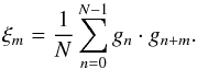 (A.1)The real-space field
components are calculated from the Fourier components by
(A.1)The real-space field
components are calculated from the Fourier components by 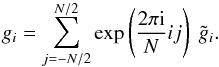 (A.2)Here, we set
 , which is equivalent to the
field having zero mean in real space. Discretization and periodicity already imply
, which is equivalent to the
field having zero mean in real space. Discretization and periodicity already imply
 – still, in order not to give double weight to this mode, we set it to zero as well. Of
course, we then have to do the same in our new method, i.e.
PN/2 ≡ 0. Note that
for the sake of readability, we still include this term in the formulae of this work.
– still, in order not to give double weight to this mode, we set it to zero as well. Of
course, we then have to do the same in our new method, i.e.
PN/2 ≡ 0. Note that
for the sake of readability, we still include this term in the formulae of this work.
Our new method draws a realization of the power spectrum and Fourier transforms it to
obtain the correlation function:  (A.3)In both methods, the
variance
(A.3)In both methods, the
variance  of the field components
in Fourier space is determined by the power spectrum, namely, for one realization,
of the field components
in Fourier space is determined by the power spectrum, namely, for one realization,
 (A.4)To prove the
equivalence of the two methods, we insert the Fourier transforms as given in Eq. (A.2) into the estimator, Eq. (A.1):
(A.4)To prove the
equivalence of the two methods, we insert the Fourier transforms as given in Eq. (A.2) into the estimator, Eq. (A.1):
 (A.5)The
sum over n simply gives a Kronecker δ, since
(A.5)The
sum over n simply gives a Kronecker δ, since
 (A.6)Thus, we obtain
 (A.7)where
in the last step, we used the fact that the
gi are real, implying
(A.7)where
in the last step, we used the fact that the
gi are real, implying
 .
In order to show that this is equivalent to Eq. (A.3), we now split the sum into two parts, omitting the zero term
(since , as we explained before):
.
In order to show that this is equivalent to Eq. (A.3), we now split the sum into two parts, omitting the zero term
(since , as we explained before):
 (A.8)Inserting
Eq. (A.4) we end up with
(A.8)Inserting
Eq. (A.4) we end up with
 (A.9)This is exactly
the way we calculate ξm in our new method –
thus, we proved analytically that the two methods are indeed equivalent. As mentioned
before, we also confirmed this fact numerically.
(A.9)This is exactly
the way we calculate ξm in our new method –
thus, we proved analytically that the two methods are indeed equivalent. As mentioned
before, we also confirmed this fact numerically.
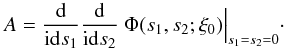
Appendix B: Analytical calculation of the ξ0-dependence of mean and covariance matrix
As mentioned in , our analytical calculation of the ξ0-dependence of the mean and the covariance matrix does not produce practically usable results – nonetheless, it is interesting from a theoretical point of view and is thus presented in this appendix.
We are ultimately interested in the mean y and the covariance matrix Cy, however, we will first show calculations in ξ-space before addressing the problem of how to transform the results to y-space.
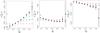 |
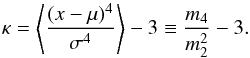
Fig. B.1 Mean of ξn for different n as function of ξ0, determined from simulations (black points with error bars) and analytically to zeroth (red crosses), first (blue circles), second (green filled triangles; left panel only), third (purple empty triangles; left panel only), and tenth (brown squares) order. |
Appendix B.1: Calculation in ξ-space
The ξ0-dependence of the mean
⟨ ξ1 ⟩ (where the index is purely a numbering and does
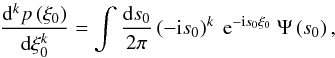
not denote the lag) can be computed as 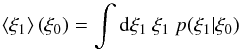 (B.1)with the
conditional probability
(B.1)with the
conditional probability  (B.2)We define the
corresponding characteristic function as Fourier transform of the probability
distribution (Φ ↔ p in short-hand notation; for details on
characteristic functions see Keitel & Schneider
2011, hereafter KS2011, and references therein):
(B.2)We define the
corresponding characteristic function as Fourier transform of the probability
distribution (Φ ↔ p in short-hand notation; for details on
characteristic functions see Keitel & Schneider
2011, hereafter KS2011, and references therein): 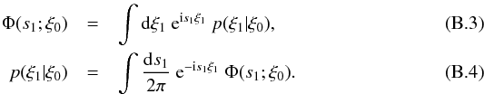 Making
use of the characteristic function
Ψ(s0,s1)
(where
Ψ(s0,s1) ↔ p(ξ0,ξ1))
computed in KS2011, we can also write
Making
use of the characteristic function
Ψ(s0,s1)
(where
Ψ(s0,s1) ↔ p(ξ0,ξ1))
computed in KS2011, we can also write
 (B.5)Comparison
with Eq. (B.3) yields
(B.5)Comparison
with Eq. (B.3) yields  (B.6)Now, we can
calculate the mean (i.e. the first moment) from the characteristic function
(equivalent to Eq. (B.1) – again, see
KS2011 and references there):
(B.6)Now, we can
calculate the mean (i.e. the first moment) from the characteristic function
(equivalent to Eq. (B.1) – again, see
KS2011 and references there): 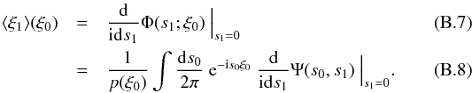 Using
the result from KS2011 for the bivariate characteristic function,
Using
the result from KS2011 for the bivariate characteristic function,
 (B.9)where
 , we can calculate the
derivative as
, we can calculate the
derivative as 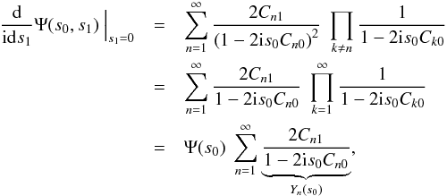 (B.10)where
we inserted the univariate characteristic function computed in KS2011,
(B.10)where
we inserted the univariate characteristic function computed in KS2011,
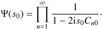 (B.11)To calculate the
integral in Eq. (B.7), we use a Taylor
expansion of
Yn(s0) from
Eq. (B.10):
(B.11)To calculate the
integral in Eq. (B.7), we use a Taylor
expansion of
Yn(s0) from
Eq. (B.10): 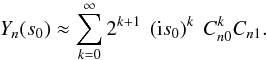 (B.12)We insert the
derivative into Eq. (B.7) and thus
obtain
(B.12)We insert the
derivative into Eq. (B.7) and thus
obtain 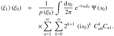 (B.13)According
to the definition of
Ψ(s0) ↔ p(ξ0),
(B.13)According
to the definition of
Ψ(s0) ↔ p(ξ0),
 (B.14)and thus, after
changing the order of summation and integration, Eq. (B.13) can finally be written as
(B.14)and thus, after
changing the order of summation and integration, Eq. (B.13) can finally be written as 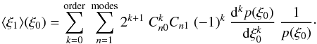 (B.15)Inserting the known
result for p(ξ0) and calculating its
derivatives allows us to compare the analytical result to simulations. The results can
be seen in ; here, the black points with error bars show the mean of
ξn for different lags
n as determined from simulations (100 000 realizations, Gaussian
power spectrum with Lk0 = 100), and the
colored symbols show the analytical results to different order (see figure caption).
It seems that, although the Taylor series in Eq. (B.15) does not converge, a truncation at order 10 yields
sufficient accuracy, barring some numerical issues for very low
ξ0-values.
(B.15)Inserting the known
result for p(ξ0) and calculating its
derivatives allows us to compare the analytical result to simulations. The results can
be seen in ; here, the black points with error bars show the mean of
ξn for different lags
n as determined from simulations (100 000 realizations, Gaussian
power spectrum with Lk0 = 100), and the
colored symbols show the analytical results to different order (see figure caption).
It seems that, although the Taylor series in Eq. (B.15) does not converge, a truncation at order 10 yields
sufficient accuracy, barring some numerical issues for very low
ξ0-values.
 |
Fig. B.2 Different elements of the covariance matrix C({ ξn }), determined from simulations (black points with error bars) and analytically to zeroth (red crosses), first (blue circles), fifth (purple triangles), and tenth (brown squares) order. |
The ξ0-dependence of the covariance matrix
Cξ can be calculated in a similar way.
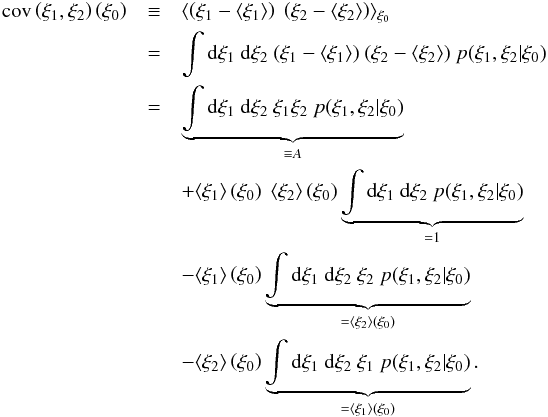
We start from the general definition of covariance,
 The
integral A can again be expressed in terms of the characteristic
function
Φ(s1,s2;ξ0) ↔ p(ξ1,ξ2 | ξ0):
The
integral A can again be expressed in terms of the characteristic
function
Φ(s1,s2;ξ0) ↔ p(ξ1,ξ2 | ξ0):
 (B.16)Similar to the
previous calculations,
(B.16)Similar to the
previous calculations, 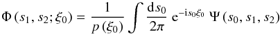 (B.17)with
the trivariate characteristic function
(B.17)with
the trivariate characteristic function 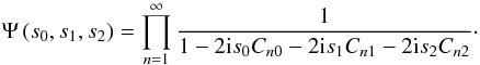 (B.18)Calculating the
second derivative of B.18 yields
(B.18)Calculating the
second derivative of B.18 yields
![Mathematical equation: \appendix \setcounter{section}{2} \begin{eqnarray} \frac{\dd}{\im\dd s_1}\frac{\dd}{\im\dd s_2} &\Psi& \left(s_0,s_1,s_2\right)\Big|_{s_1=s_2=0}= \nonumber\\ && \Psi\left(s_0\right) \left[\sum_{n=1}^\infty \underbrace{\frac{4\Cnone\Cntwo}{(1-2\im s_0\Cnzero)^2}}_{Z_n(s_0)} \right.\nonumber\\ &&+ \left. \sum_{n,k=1}^\infty \underbrace{\frac{4\Cnone\Cktwo}{(1-2\im s_0\Cnzero)(1-2\im s_0\Ckzero)}}_{Z_{k,n}(s_0)} \right]\cdot \end{eqnarray}](/articles/aa/full_html/2013/08/aa21718-13/aa21718-13-eq257.png) (B.19)The
Taylor expansions of
Zn(s0) and
Zk,n(s0)
read
(B.19)The
Taylor expansions of
Zn(s0) and
Zk,n(s0)
read 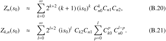 Using
it as well as the expansion (B.12), we
finally obtain
Using
it as well as the expansion (B.12), we
finally obtain ![Mathematical equation: \appendix \setcounter{section}{2} \begin{eqnarray} \label{eq:cov_xi_final} \cov\left(\xi_1,\xi_2\right)\left(\xi_0\right) &=& \sum_{k=0}^\mathrm{order}\ \frac{1}{p(\xi_0)}\frac{\dd^k p\left(\xi_0\right)}{\dd\xi_0^k} \left[ \sum_{n}^\mathrm{modes} (-1)^k\ 2^{k+2}\ (k+1)\right.\nonumber\\ &&\times \Cnzero^k\Cnone\Cntwo + \sum_{n,m}^\mathrm{modes} (-1)^k\ 2^{k+2}\ \Cmtwo\ \Cnone\nonumber\\ &&\times \left. \sum_{p=0}^{k}\Cmzero^p\ \Cnzero^{k-p} \right] - \langle\xi_1\rangle(\xi_0)\ \langle\xi_2\rangle(\xi_0). \end{eqnarray}](/articles/aa/full_html/2013/08/aa21718-13/aa21718-13-eq261.png) (B.22)We
show a comparison of the results (for different elements of the covariance matrix)
from simulations and the analytical formula in . Again, the black dots are obtained
from simulations and the colored symbols represent the results from Eq. (B.22), where the last term (i.e. the one
containing the mean values ⟨ ξn ⟩) was
calculated up to tenth order, thus providing sufficient accuracy, as previously shown.
As before, there are some numerical problems for very small values of
ξ0. Additionally, the analytical results do not agree
with the simulations for small lags, as can be seen from the left-most panel (the same
holds for other covariance matrix elements involving small lags). However, for the the
higher-lag examples (i.e. the right two panels), a truncation of the Taylor series at
tenth order seems to be accurate enough.
(B.22)We
show a comparison of the results (for different elements of the covariance matrix)
from simulations and the analytical formula in . Again, the black dots are obtained
from simulations and the colored symbols represent the results from Eq. (B.22), where the last term (i.e. the one
containing the mean values ⟨ ξn ⟩) was
calculated up to tenth order, thus providing sufficient accuracy, as previously shown.
As before, there are some numerical problems for very small values of
ξ0. Additionally, the analytical results do not agree
with the simulations for small lags, as can be seen from the left-most panel (the same
holds for other covariance matrix elements involving small lags). However, for the the
higher-lag examples (i.e. the right two panels), a truncation of the Taylor series at
tenth order seems to be accurate enough.
Appendix B.2: Transformation of mean and covariance matrix to y-space
In the previous section, we showed how to calculate the (ξ0-dependent) mean and covariance matrix in ξ-space. The computation of the quasi-Gaussian approximation, however, requires the mean y and the covariance matrix Cy in y-space, which cannot be obtained from those in ξ-space in a trivial way due to the highly non-linear nature of the transformation ξ → y.
Thus, instead of settling for a linear approximation, we have to choose a more
computationally expensive approach. Namely, we calculate the first and second moments
(in ξ) of the quasi-Gaussian distribution as functions of the mean
and (inverse) covariance matrix in y-space and equate the result to
the analytical results, i.e. we solve a set of equation of the form
 where
we did not write down the ξ0-dependence explicitly for the
sake of readability.
where
we did not write down the ξ0-dependence explicitly for the
sake of readability.
Note that this is a complicated procedure, since the integration on the equations’ left-hand sides can only be performed
numerically (we make use of a Monte-Carlo code from Press et al. 2007). In order to solve the equation set (consisting of
 equation for an
N-variate distribution) we use a multi-dimensional root-finding
algorithm (as provided within the GSL, Galassi et al.
2009). However, due to the high dimensionality of the problem, this procedure
does not seem practical, since it is computationally very expensive – in addition to
that, any possible gain in accuracy is averted by the required heavy use of purely
numerical methods.
equation for an
N-variate distribution) we use a multi-dimensional root-finding
algorithm (as provided within the GSL, Galassi et al.
2009). However, due to the high dimensionality of the problem, this procedure
does not seem practical, since it is computationally very expensive – in addition to
that, any possible gain in accuracy is averted by the required heavy use of purely
numerical methods.
Thus, as described in , we refrain from using our analytical results for the mean and covariance matrix and simply determine them (as well as their ξ0-dependence) from simulations, which we have shown to be sufficiently accurate.
Acknowledgments
We would like to thank Cristiano Porciani, David Keitel, and Jan Hartlap for useful help and discussion in the course of the project as well as Benjamin Joachimi for providing his Box-Cox code. We also thank our anonymous referee for constructive comments and suggestions. This work was supported by the Deutsche Forschungsgemeinschaft under the project SCHN 342/11.
References
- Box, G. E. P., & Cox, D. R. 1964, J. Roy. Statist. Soc. Ser. B (Methodological), 26, 211 [Google Scholar]
- Carron, J. 2013, A&A, 551, A88 [NASA ADS] [CrossRef] [EDP Sciences] [Google Scholar]
- Galassi, M., Davies, J., Theiler, J., et al. 2009, GNU Scientific Library Reference Manual, 3rd edn (Network Theory Ltd.) [Google Scholar]
- Hartlap, J., Schrabback, T., Simon, P., & Schneider, P. 2009, A&A, 504, 689 [NASA ADS] [CrossRef] [EDP Sciences] [Google Scholar]
- Henze, N. 2002, Statistical Papers, 43, 467 [CrossRef] [Google Scholar]
- Joachimi, B., Taylor, A. N., & Kiessling, A. 2011, MNRAS, 418, 145 [NASA ADS] [CrossRef] [Google Scholar]
- Joe, S., & Kuo, F. Y. 2008, SIAM J. Sci. Comput., 30, 2635 [CrossRef] [Google Scholar]
- Keitel, D., & Schneider, P. 2011, A&A, 534, A76 [NASA ADS] [CrossRef] [EDP Sciences] [Google Scholar]
- Labatie, A., Starck, J.-L., & Lachièze-Rey, M. 2012a, ApJ, 746, 172 [NASA ADS] [CrossRef] [Google Scholar]
- Labatie, A., Starck, J.-L., & Lachièze-Rey, M. 2012b, ApJ, 760, 97 [NASA ADS] [CrossRef] [Google Scholar]
- Mardia, K. 1970, Biometrika, 57, 519 [CrossRef] [Google Scholar]
- Mardia, K. 1974, Sankhyā Series B. Methodological, 36, 115 [Google Scholar]
- Press, W. H., Teukolsky, S. A., Vetterling, W. T., & Flannery, B. P. 2007, Numerical Recipes 3rd edn, The Art of Scientific Computing (New York, NY, USA: Cambridge University Press) [Google Scholar]
- Sato, M., Ichiki, K., & Takeuchi, T. T. 2010, Phys. Rev. Lett., 105, 251301 [NASA ADS] [CrossRef] [Google Scholar]
- Sato, M., Ichiki, K., & Takeuchi, T. T. 2011, Phys. Rev. D, 83, 023501 [NASA ADS] [CrossRef] [Google Scholar]
- Scherrer, R. J., Berlind, A. A., Mao, Q., & McBride, C. K. 2010, ApJ, 708, L9 [Google Scholar]
- Schneider, P., & Hartlap, J. 2009, A&A, 504, 705 [NASA ADS] [CrossRef] [EDP Sciences] [Google Scholar]
- Seljak, U., & Bertschinger, E. 1993, ApJ, 417, L9 [NASA ADS] [CrossRef] [Google Scholar]
- Sun, L., Wang, Q., & Zhan, H. 2013, ApJ, submitted [arXiv:1306.5064] [Google Scholar]
All Figures
|
Fig. 1 Constraints in the r3-r4-plane (i.e. with fixed r1 and r2) for a field with N = 16 grid points and randomly drawn power spectra. For the lower bound, the results from the Cauchy-Schwarz inequality (green) as well as from the covariance matrix approach (blue) are shown. |
| In the text | |
|
Fig. 2 Iso-probability contours of p(ξ3,ξ6) (left) and p(y3,y6) (right) for 400 000 realizations of a field with N = 32 grid points and a Gaussian power spectrum with Lk0 = 80. The dashed red contours show the best-fitting Gaussian approximations in both cases. |
| In the text | |
|
Fig. 3 p(r1,r2) for a field with N = 32 grid points and a Gaussian power spectrum with Lk0 = 80. The dashed red contours show the transformed Gaussian approximation from y-space. |
| In the text | |
|
Fig. 4 p(ξ0) for a random field with N = 32 grid points and a Gaussian power spectrum with Lk0 = 80: the black dots show the PDF from the simulation, whereas the red curve was calculated from the analytical formula, using N/2−1 = 15 modes and the same field length and power spectrum. |
| In the text | |
|
Fig. 5 p(ξ1,ξ2) for a field with N = 32 grid points and a Gaussian power spectrum with Lk0 = 80. The dashed red contours show the transformed Gaussian approximation from y-space. |
| In the text | |
|
Fig. 6 Mean (top row) and standard deviation (second row) of yn for different n as well as different off-diagonal elements of the covariance matrix C(⟨ yn ⟩) (third row) as functions of ξ0, determined from simulations; the error bars show the corresponding standard errors (which depend on the number of realizations with a value of ξ0 that lies in the current bin). |
| In the text | |
|
Fig. 7 Skewness (left-hand panel) and kurtosis (right-hand panel) of { ξn } (black circles) and { yn } (red triangles) as functions of lag n, for a Gaussian power spectrum with Lk0 = 80. The blue squares show the skewness/kurtosis of Gaussian samples of the same length, mean and variance as the corresponding samples { yn }. |
| In the text | |
|
Fig. 8 Mardia’s skewness (left-hand panel) and kurtosis (right-hand panel) of n-variate { ξ }- (black circles) and { y }-samples (red, upward triangles) for a Gaussian power spectrum with Lk0 = 80. The green, downward triangles show the skewness/kurtosis of { y }-samples obtained under the assumption of a Gaussian { ξ }-sample, and the blue squares show the skewness/kurtosis of Gaussian samples. See text for more details. |
| In the text | |
|
Fig. 9 p(ξ1) for a field with N = 32 grid points and a Gaussian power spectrum with Lk0 = 80. The black curve is from simulations, the blue dot-dashed curve shows the best-fitting Gaussian, and the other two curves show the quasi-Gaussian approximation using a constant covariance matrix (green dotted curve) and incorporating its ξ0-dependence (red dashed curve). |
| In the text | |
|
Fig. 10 Posterior probability for the power spectrum parameters
|
| In the text | |
|
Fig. 11 Marginalized posterior probabilities for the power spectrum parameters A and k0. The solid black curves are the results obtained from the Gaussian likelihood, whereas the red dot-dashed curves show the results from the quasi-Gaussian analysis. |
| In the text | |
|
Fig. 12 p(ξ1,ξ2) (left) and p(ξ3,ξ6) (right) for a field with N = 32 grid points and a Gaussian power spectrum with Lk0 = 80. The dashed red contours show the approximation obtained from a Gaussian copula. |
| In the text | |
|
Fig. B.1 Mean of ξn for different n as function of ξ0, determined from simulations (black points with error bars) and analytically to zeroth (red crosses), first (blue circles), second (green filled triangles; left panel only), third (purple empty triangles; left panel only), and tenth (brown squares) order. |
| In the text | |
|
Fig. B.2 Different elements of the covariance matrix C({ ξn }), determined from simulations (black points with error bars) and analytically to zeroth (red crosses), first (blue circles), fifth (purple triangles), and tenth (brown squares) order. |
| In the text | |
Current usage metrics show cumulative count of Article Views (full-text article views including HTML views, PDF and ePub downloads, according to the available data) and Abstracts Views on Vision4Press platform.
Data correspond to usage on the plateform after 2015. The current usage metrics is available 48-96 hours after online publication and is updated daily on week days.
Initial download of the metrics may take a while.