| Issue |
A&A
Volume 556, August 2013
|
|
|---|---|---|
| Article Number | A70 | |
| Number of page(s) | 16 | |
| Section | Cosmology (including clusters of galaxies) | |
| DOI | https://doi.org/10.1051/0004-6361/201321718 | |
| Published online | 30 July 2013 | |
Online material
Appendix A: Equivalence of the simulation methods
In this appendix, we want to prove analytically that the two simulation methods mentioned in are in fact equivalent.
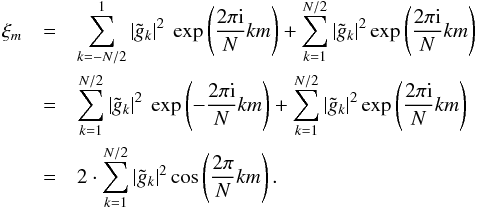
The established method calculates the correlation function components
ξm,
m = 0,..., N − 1
directly from the field components gn,
n = 0,..., N − 1.
Since we impose periodic boundary conditions on the field, this can be done using the
estimator  (A.1)The real-space field
components are calculated from the Fourier components by
(A.1)The real-space field
components are calculated from the Fourier components by  (A.2)Here, we set
 , which is equivalent to the
field having zero mean in real space. Discretization and periodicity already imply
, which is equivalent to the
field having zero mean in real space. Discretization and periodicity already imply
 – still, in order not to give double weight to this mode, we set it to zero as well. Of
course, we then have to do the same in our new method, i.e.
PN/2 ≡ 0. Note that
for the sake of readability, we still include this term in the formulae of this work.
– still, in order not to give double weight to this mode, we set it to zero as well. Of
course, we then have to do the same in our new method, i.e.
PN/2 ≡ 0. Note that
for the sake of readability, we still include this term in the formulae of this work.
Our new method draws a realization of the power spectrum and Fourier transforms it to
obtain the correlation function:  (A.3)In both methods, the
variance
(A.3)In both methods, the
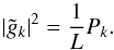
variance  of the field components
in Fourier space is determined by the power spectrum, namely, for one realization,
of the field components
in Fourier space is determined by the power spectrum, namely, for one realization,
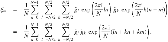
 (A.4)To prove the
equivalence of the two methods, we insert the Fourier transforms as given in Eq. (A.2) into the estimator, Eq. (A.1):
(A.4)To prove the
equivalence of the two methods, we insert the Fourier transforms as given in Eq. (A.2) into the estimator, Eq. (A.1):
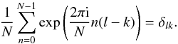
 (A.5)The
sum over n simply gives a Kronecker δ, since
(A.5)The
sum over n simply gives a Kronecker δ, since
 (A.6)Thus, we obtain
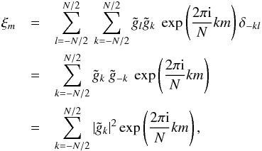 (A.7)where
in the last step, we used the fact that the
gi are real, implying
(A.7)where
in the last step, we used the fact that the
gi are real, implying
 .
In order to show that this is equivalent to Eq. (A.3), we now split the sum into two parts, omitting the zero term
(since , as we explained before):
.
In order to show that this is equivalent to Eq. (A.3), we now split the sum into two parts, omitting the zero term
(since , as we explained before):
 (A.8)Inserting
Eq. (A.4) we end up with
(A.8)Inserting
Eq. (A.4) we end up with
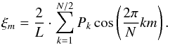 (A.9)This is exactly
the way we calculate ξm in our new method –
thus, we proved analytically that the two methods are indeed equivalent. As mentioned
before, we also confirmed this fact numerically.
(A.9)This is exactly
the way we calculate ξm in our new method –
thus, we proved analytically that the two methods are indeed equivalent. As mentioned
before, we also confirmed this fact numerically.
Appendix B: Analytical calculation of the ξ0-dependence of mean and covariance matrix
As mentioned in , our analytical calculation of the ξ0-dependence of the mean and the covariance matrix does not produce practically usable results – nonetheless, it is interesting from a theoretical point of view and is thus presented in this appendix.
We are ultimately interested in the mean y and the covariance matrix Cy, however, we will first show calculations in ξ-space before addressing the problem of how to transform the results to y-space.
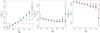 |
Fig. B.1
Mean of ξn for different n as function of ξ0, determined from simulations (black points with error bars) and analytically to zeroth (red crosses), first (blue circles), second (green filled triangles; left panel only), third (purple empty triangles; left panel only), and tenth (brown squares) order. |
| Open with DEXTER | |
Appendix B.1: Calculation in ξ-space
The ξ0-dependence of the mean
⟨ ξ1 ⟩ (where the index is purely a numbering and does
not denote the lag) can be computed as 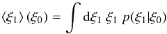 (B.1)with the
conditional probability
(B.1)with the
conditional probability 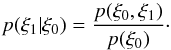 (B.2)We define the
corresponding characteristic function as Fourier transform of the probability
distribution (Φ ↔ p in short-hand notation; for details on
characteristic functions see Keitel & Schneider
2011, hereafter KS2011, and references therein):
(B.2)We define the
corresponding characteristic function as Fourier transform of the probability
distribution (Φ ↔ p in short-hand notation; for details on
characteristic functions see Keitel & Schneider
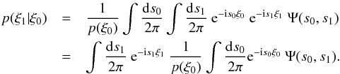
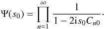
2011, hereafter KS2011, and references therein): 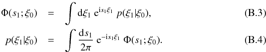 Making
use of the characteristic function
Ψ(s0,s1)
(where
Ψ(s0,s1) ↔ p(ξ0,ξ1))
computed in KS2011, we can also write
Making
use of the characteristic function
Ψ(s0,s1)
(where
Ψ(s0,s1) ↔ p(ξ0,ξ1))
computed in KS2011, we can also write
 (B.5)Comparison
with Eq. (B.3) yields
(B.5)Comparison
with Eq. (B.3) yields 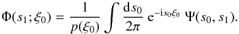 (B.6)Now, we can
calculate the mean (i.e. the first moment) from the characteristic function
(equivalent to Eq. (B.1) – again, see
KS2011 and references there):
(B.6)Now, we can
calculate the mean (i.e. the first moment) from the characteristic function
(equivalent to Eq. (B.1) – again, see
KS2011 and references there): 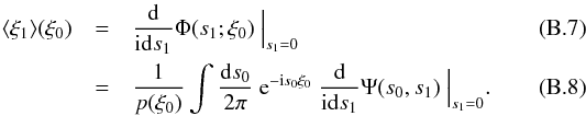 Using
the result from KS2011 for the bivariate characteristic function,
Using
the result from KS2011 for the bivariate characteristic function,
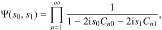 (B.9)where
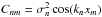 , we can calculate the
derivative as
, we can calculate the
derivative as 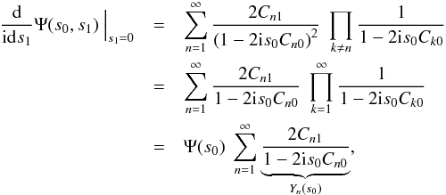 (B.10)where
we inserted the univariate characteristic function computed in KS2011,
(B.10)where
we inserted the univariate characteristic function computed in KS2011,
 (B.11)To calculate the
integral in Eq. (B.7), we use a Taylor
expansion of
Yn(s0) from
Eq. (B.10):
(B.11)To calculate the
integral in Eq. (B.7), we use a Taylor
expansion of
Yn(s0) from
Eq. (B.10): 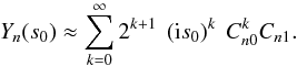 (B.12)We insert the
derivative into Eq. (B.7) and thus
obtain
(B.12)We insert the
derivative into Eq. (B.7) and thus
obtain 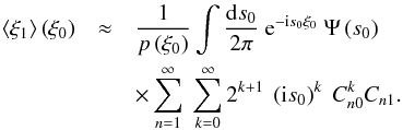 (B.13)According
to the definition of
Ψ(s0) ↔ p(ξ0),
(B.13)According
to the definition of
Ψ(s0) ↔ p(ξ0),
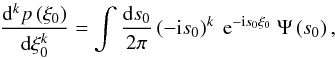 (B.14)and thus, after
changing the order of summation and integration, Eq. (B.13) can finally be written as
(B.14)and thus, after
changing the order of summation and integration, Eq. (B.13) can finally be written as 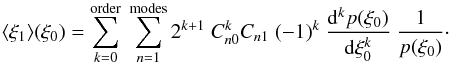 (B.15)Inserting the known
result for p(ξ0) and calculating its
derivatives allows us to compare the analytical result to simulations. The results can
be seen in ; here, the black points with error bars show the mean of
ξn for different lags
n as determined from simulations (100 000 realizations, Gaussian
power spectrum with Lk0 = 100), and the
colored symbols show the analytical results to different order (see figure caption).
It seems that, although the Taylor series in Eq. (B.15) does not converge, a truncation at order 10 yields
sufficient accuracy, barring some numerical issues for very low
ξ0-values.
(B.15)Inserting the known
result for p(ξ0) and calculating its
derivatives allows us to compare the analytical result to simulations. The results can
be seen in ; here, the black points with error bars show the mean of
ξn for different lags
n as determined from simulations (100 000 realizations, Gaussian
power spectrum with Lk0 = 100), and the
colored symbols show the analytical results to different order (see figure caption).
It seems that, although the Taylor series in Eq. (B.15) does not converge, a truncation at order 10 yields
sufficient accuracy, barring some numerical issues for very low
ξ0-values.
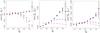 |
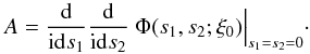
Fig. B.2
Different elements of the covariance matrix C({ ξn }), determined from simulations (black points with error bars) and analytically to zeroth (red crosses), first (blue circles), fifth (purple triangles), and tenth (brown squares) order. |
| Open with DEXTER | |
The ξ0-dependence of the covariance matrix
Cξ can be calculated in a similar way.
We start from the general definition of covariance,
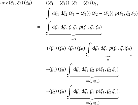 The
integral A can again be expressed in terms of the characteristic
function
Φ(s1,s2;ξ0) ↔ p(ξ1,ξ2 | ξ0):
The
integral A can again be expressed in terms of the characteristic
function
Φ(s1,s2;ξ0) ↔ p(ξ1,ξ2 | ξ0):
 (B.16)Similar to the
previous calculations,
(B.16)Similar to the
previous calculations, 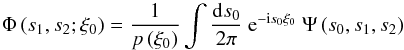 (B.17)with
the trivariate characteristic function
(B.17)with
the trivariate characteristic function 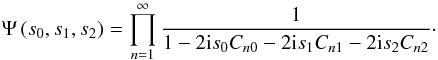 (B.18)Calculating the
second derivative of B.18 yields
(B.18)Calculating the
second derivative of B.18 yields
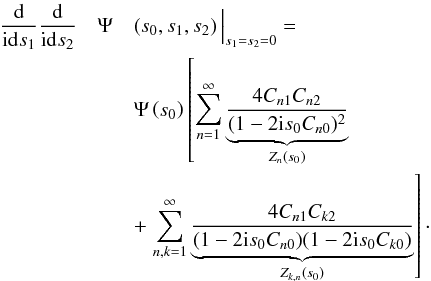 (B.19)The
Taylor expansions of
Zn(s0) and
Zk,n(s0)
read
(B.19)The
Taylor expansions of
Zn(s0) and
Zk,n(s0)
read 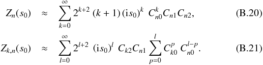 Using
it as well as the expansion (B.12), we
finally obtain
Using
it as well as the expansion (B.12), we
finally obtain 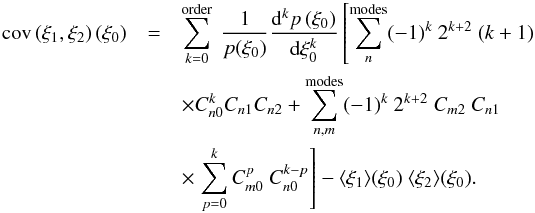 (B.22)We
show a comparison of the results (for different elements of the covariance matrix)
from simulations and the analytical formula in . Again, the black dots are obtained
from simulations and the colored symbols represent the results from Eq. (B.22), where the last term (i.e. the one
containing the mean values ⟨ ξn ⟩) was
calculated up to tenth order, thus providing sufficient accuracy, as previously shown.
As before, there are some numerical problems for very small values of
ξ0. Additionally, the analytical results do not agree
with the simulations for small lags, as can be seen from the left-most panel (the same
holds for other covariance matrix elements involving small lags). However, for the the
higher-lag examples (i.e. the right two panels), a truncation of the Taylor series at
tenth order seems to be accurate enough.
(B.22)We
show a comparison of the results (for different elements of the covariance matrix)
from simulations and the analytical formula in . Again, the black dots are obtained
from simulations and the colored symbols represent the results from Eq. (B.22), where the last term (i.e. the one
containing the mean values ⟨ ξn ⟩) was
calculated up to tenth order, thus providing sufficient accuracy, as previously shown.
As before, there are some numerical problems for very small values of
ξ0. Additionally, the analytical results do not agree
with the simulations for small lags, as can be seen from the left-most panel (the same
holds for other covariance matrix elements involving small lags). However, for the the
higher-lag examples (i.e. the right two panels), a truncation of the Taylor series at
tenth order seems to be accurate enough.
Appendix B.2: Transformation of mean and covariance matrix to y-space
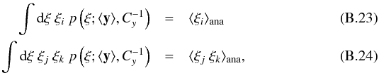
In the previous section, we showed how to calculate the (ξ0-dependent) mean and covariance matrix in ξ-space. The computation of the quasi-Gaussian approximation, however, requires the mean y and the covariance matrix Cy in y-space, which cannot be obtained from those in ξ-space in a trivial way due to the highly non-linear nature of the transformation ξ → y.
Thus, instead of settling for a linear approximation, we have to choose a more
computationally expensive approach. Namely, we calculate the first and second moments
(in ξ) of the quasi-Gaussian distribution as functions of the mean
and (inverse) covariance matrix in y-space and equate the result to
the analytical results, i.e. we solve a set of equation of the form
 where
we did not write down the ξ0-dependence explicitly for the
sake of readability.
where
we did not write down the ξ0-dependence explicitly for the
sake of readability.
Note that this is a complicated procedure, since the integration on the equations’ left-hand sides can only be performed
numerically (we make use of a Monte-Carlo code from Press et al. 2007). In order to solve the equation set (consisting of
 equation for an
N-variate distribution) we use a multi-dimensional root-finding
algorithm (as provided within the GSL, Galassi et al.
2009). However, due to the high dimensionality of the problem, this procedure
does not seem practical, since it is computationally very expensive – in addition to
that, any possible gain in accuracy is averted by the required heavy use of purely
numerical methods.
equation for an
N-variate distribution) we use a multi-dimensional root-finding
algorithm (as provided within the GSL, Galassi et al.
2009). However, due to the high dimensionality of the problem, this procedure
does not seem practical, since it is computationally very expensive – in addition to
that, any possible gain in accuracy is averted by the required heavy use of purely
numerical methods.
Thus, as described in , we refrain from using our analytical results for the mean and covariance matrix and simply determine them (as well as their ξ0-dependence) from simulations, which we have shown to be sufficiently accurate.
© ESO, 2013
Current usage metrics show cumulative count of Article Views (full-text article views including HTML views, PDF and ePub downloads, according to the available data) and Abstracts Views on Vision4Press platform.
Data correspond to usage on the plateform after 2015. The current usage metrics is available 48-96 hours after online publication and is updated daily on week days.
Initial download of the metrics may take a while.