| Issue |
A&A
Volume 556, August 2013
|
|
|---|---|---|
| Article Number | A153 | |
| Number of page(s) | 18 | |
| Section | Astrophysical processes | |
| DOI | https://doi.org/10.1051/0004-6361/201321292 | |
| Published online | 09 August 2013 | |
On the origin of non-self-gravitating filaments in the ISM⋆
1 Laboratoire AIM, Paris-Saclay, CEA/IRFU/SAp − CNRS − Université Paris Diderot, 91191 Gif-sur-Yvette Cedex, France
e-mail: This email address is being protected from spambots. You need JavaScript enabled to view it.
2 LERMA (UMR CNRS 8112), École Normale Supérieure, 75231 Paris Cedex, France
Received: 14 February 2013
Accepted: 18 June 2013
Abstract
Context. Filaments are ubiquitous in the interstellar medium, as recently emphasized by Herschel, yet their physical origin remains elusive
Aims. It is therefore important to understand the physics of molecular clouds to investigate how filaments form and which role play various processes, such as turbulence and magnetic field.
Methods. We used ideal magnetohydrodynamic (MHD) simulations to study the formation of clumps in various conditions, including different magnetization and Mach numbers as well as two completely different setups. We then performed several analyses to compute the shape of the clumps and their link to velocities and forces using various approaches.
Results. We found that on average, clumps in MHD simulations are more filamentary than clumps in hydrodynamical simulations. Detailed analyses reveal that the filaments are in general preferentially aligned with the strain, which means that these structures simply result from the stretch induced by turbulence. Moreover, filaments tend to be confined by the Lorentz force, which therefore leads them to survive longer in magnetized flows. We show that in all simulations they have a typical thickness equal to a few grid cells, suggesting that they are primarily associated to the energy dissipation within the flow. We estimate the order of magnitude of the dissipation length associated to the ion-neutral friction and conclude that in well UV shielded regions it is about 0.1 pc and therefore could possibly set the typical size of non-self-gravitating filaments.
Conclusions. Filaments are ubiquitous because they are the results of the very generic turbulent strain and because the magnetic field helps to keep them coherent. We suggest that energy dissipation is playing a determining role in their formation.
Key words: turbulence / magnetic fields / ISM: structure / ISM: kinematics and dynamics / ISM: clouds / stars: formation
Appendices are available in electronic form at http://www.aanda.org
© ESO, 2013
1. Introduction
After more than three decades of research, the evidence for the filamentary structure of the molecular clouds seen through their CO emission has become clear (e.g. Ungerechts & Thaddeus 1987; Bally et al. 1987). The far-IR all-sky IRAS survey (Low et al. 1984) also revealed the ubiquitous filamentary structure of the diffuse interstellar medium (ISM), and discovered the cirrus clouds, i.e., the filamentary structure of the ISM.
Thanks to its unprecedented sensitivity and large-scale mapping capabilities, the satellite Herschel has now provided a unique view of these filamentary structures of cold dust (e.g. Miville-Deschênes et al. 2010; Ward-Thompson et al. 2010; André et al. 2010). One of the main and intriguing findings is the very wide range of column densities – a factor of 100 between the most tenuous (NH2 = 2 × 1020 cm-2) and most opaque (NH2 ~ 1023 cm-2) of the observed filaments in several fields, contrasting with a narrow range of filament thickness (between 0.03 and 0.2 pc) that is barely increasing with the central column density (Arzoumanian et al. 2011). The present study is largely motivated by this result, though as described below, it is too early to conclude.
While the filamentary nature of molecular clouds is probably linked to their turbulence, the exact mechanism by which this happens remains to be understood. In many published numerical simulations, filaments are clearly present (e.g. de Avillez & Breitschwerdt 2005; Heitsch et al. 2005; Joung & MacLow 2006; Padoan et al. 2007; Hennebelle et al. 2008; Price & Bate 2008; Banerjee et al. 2009; Inoue et al. 2009; Nakamura & Li 2008; Seifreid et al. 2011; Vázquez-Semadeni et al. 2011; Federrath & Klessen 2013), but again the exact reason of their formation mechanism is not very clearly analyzed. Based on the evidence for higher velocities in the outer part of the filaments, Padoan et al. (2001) proposed that filaments form through the collision of two shocked sheets. Another explanation invokes instabilities in self-gravitating sheets (e.g. Nagai et al. 1998). Although it is clear that since filaments are denser than their environment, some compression must necessarily occur, it is important to understand the conditions in which the filament formation happens in greater detail. An important question, in particular, is the origin of the elongation. Is the elongation produced by the contraction along two directions, as would happen in a shock or in a converging flow? Or is the elongation the result of the stretching of the fluid particles along one direction? The purpose of this paper is to investigate these questions.
The paper is organized as follows. In the second part we describe the analysis that we performed on the clumps and the filaments formed in the numerical simulations. We also describe the various runs that we carried out to understand the filament origin. In the third section, we present a simple but enlightening preliminary numerical experiment that clearly demonstrates that the mechanism we propose can actually work. In the fourth section we show the numerical simulations and present the clump statistics, such as their aspect ratio, length, and thickness distributions. In the fifth section we analyze the link between the filament orientation, the velocity field, and the forces. The sixth section provides a more detailed discussion of the filament thickness as well as simple orders of magnitude which suggest that ion-neutral friction could possibly explain their thickness. The seventh section concludes the paper.
2. General analysis and numerical simulations
2.1. Structure analysis
We perform numerical simulations relevant for the diffuse and moderately dense ISM. The mean density we consider reaches from 5 cm-3 to about 100 cm-3 while the highest densities exceed a few 103 cm-3.
2.1.1. Definitions
The first difficulty when discussing clouds is to define them. To identify structures in this work, we followed a simple approach. The first step was to choose a density threshold (two of them are used through the paper, nthres = 50 and 200 cm-3) and to clip the density field. Then using a friend-of-friend analysis, the connected cells were associated to form a clump. Subsequently, the structure properties can easily be computed. The structures obtained through this process are called clumps. In many occasions we also refer to filaments. Filaments as clumps are not well-identified objects, and although it could be easy to adopt an arbitary criterion such as an aspect ratio higher than some values, this would not yield much information. When we use the word filament simply to refer to a clump that is sufficiently elongated for instance by a factor of about 5 or more.
2.1.2. Inertia matrix
To estimate the shape of a structure, it is convenient to compute the inertia matrix and its eigenvalues and eigenvectors. The inertia matrix is a three by three matrix defined as  , where xi are the coordinates of the cells belonging to the structure associated to its center of mass. The three eigenvectors give the three main axes of the structure, which correspond to the symmetry axes if the structure, admits some, while the eigenvalues represent the moment of inertia of the structure with respect to the three eigenvectors. From the inertia momentum, Ii, we can obtain an estimate of the structure size
  , where M is the structure mass. In the case of filaments, for example, the eigenvector associated with the highest eigenvalue tends to be aligned with the main axis of the filament while the two other eigenvectors tend to be perpendicular to the filament axis. In the following, we refer to the eigenvector associated to the highest eigenvalue as the main axis. We also quantify the aspect ratio of structures by computing the ratio of eigenvalues. We consider in particular μ1/μ3 and μ2/μ3, the ratios of the smallest over the largest structure size and the intermediate over the largest, respectively.
One of the difficulties with this approach is that thin but curved filaments will have moments of inertia that reflect the curvature instead of the effective thickness. For this reason, we use a second method to characterize their shape.
2.2. Strain tensor
The strain tensor is another useful quantity that we used to perform our analysis. It was obtained by considering the velocity difference between two fluid particles located in r and r + dr. One obtains vi(r + dr) − vi(r) = ∂jvidrj, where summation over repeating indices is used. The three by three matrix, ∂jvi, can be splitted into its anti-symmetric part Ai,j = (∂jvi − ∂ivj)/2, which describes the rotation of the fluid element and its symmetric part Si,j = (∂jvi + ∂ivj)/2, which describes the shape modification of the fluid element and is called the infinitesimal strain tensor. The trace Si,i, which is equal to the divergence of v, describes the change of volume. The symmetric part can be diagolized leading to three eigenvalues, si, where we assume that s3 > s2 > s1. The eigenvector associated to the highest eigenvalue, s3, describes the axis along which the fluid particle is mostly elongated, below we call it the strain. In principle since the divergence of the fluid is non-zero, all eigenvalues could be negative, which would then correspond to a global contraction. In practice, this is almost never the case at the scale of the clump in our simulations. The two other eigenvectors associated to the two other eigenvalues correspond to the directions along which the shape of the fluid particle is either stretched or compressed, depending on their signs.
Computing the strain tensor is not straightforward since it requires one to take the velocity gradients between cells. Moreover, because of the numerical diffusion, the gradients at the scale of the mesh are artificially smoothed. To limit this problem, we smoothed the simulation by a factor three, computing the mean density-weighted velocity within the smoothed cells. Then we computed all velocity gradients using simple finite differences and computed the mean gradients by summing over all cells that belong to the structure. Finally, we used these values to compute Sij.
2.2.1. Simple skeleton-like approach
Another useful approach is determining an average line characteristic of the clump shape. This type of algorithm has been developed in the context of Cosmology to reconstruct the filaments that lead to the so-called skeleton (Sousbie et al. 2009). Here we follow a simpler approach which is well-suited for our analysis. The first step is to select the direction (x, y or z) along which the structure is the longest. Then, we can subdivide it into a number of slices, nsl, of a given length in the selected direction. Each slice, i, can itself be divided into nsr connecting regions, that is to say, regions in which all cells are connected to each other through their neighbors. Each of these subregions, j, belongs to a different branch within the structure. Then the center of mass,  of each of these subregions within each slice can be computed, leading to an ensemble of points . For each of them we look for the nearest neighbor,
  of belonging to the slices i − 1 or i + 1. Finally, we calculate the vector
  , which gives the local direction of the branch to which belongs. The sign is then chosen to insure
  , where X represents the selected axis, x, y or z. Connecting all to their respective neighbors, we obtain a curve that represents the mean local direction. Figure 1 shows an example of a clump extracted from the fiducial magnetohydrodynamic (MHD) simulation presented below. The white cells represent the position of . They follow closely each branch of the clump. The two arrows represent the clump main axis (computed with the inertia matrix as explained above) and the strain (computed with the strain tensor). Note that the clump is quite filamentary and that the main axis represented by the vertical arrow follows the filament direction well.
 |
Fig. 1 Column density and velocity field for one of the clumps formed in the MHD simulations. The white points represent the local mass center Gij and constitute the skeleton of the clump. The upward pointing arrow represents the filament main axis as computed with the inertia matrix. The downward pointing arrow represents the main direction of the strain as computed with the strain tensor. |
Once the  are known, it is an easy task to estimate the distance, rM, from a given filament cell to the skeleton. Since any cell belonging to the structure is associated to a subregion, one can calculate
  , where M is the cell center. We made use of the vectors to compute various quantities as the mean component of various forces. The mean radius is then defined as rc = ΣrMdm/Σdm, where dm is the mass within the cell and where the sum is taken over all clump cells. We stress that the thickness, rc calculated by this definition measures the thickness of the clump substructures and not the mean size of the clumps, which would take into account the distance between the various branches. This is particularly clear in Fig. 1, where the distance between the branches is on the order of a few pc while in most regions of the clump, the size of the individual branches is typically ten times smaller.
2.3. Description of numerical simulations
2.3.1. Code and resolution
We used the Ramses code (Teyssier 2002; Fromang et al. 2006) to perform the simulations. Ramses uses adaptive mesh refinement and solves the ideal MHD equations using the Riemann HLLD solver (Miyoshi & Kuzano 2005). It uses the constraint transport method to ensure that divB is maintained to be zero. The cooling corresponds to the standard ISM cooling (e.g. Wolfire et al. 1995) as described in Audit & Hennebelle (2005) and includes Lyman α, C+, and O lines. The heating is due to the photo-electric effect on small dust grains. We carried out simulations with have a based grid of 5123 cells. Then, depending on the simulations, we either added one or two other AMR levels, leading to an effective resolution in the most refined areas of 10243 to 20483 cells. The refinement criteria is based on density. Any cell with a density higher than 50 cm-3 is refined to a resolution of 10243 and when it is allowed, cells denser than 200-3 are refined to resolution 20483. The high-resolution run allows us to check for numerical convergence and to verify by comparison with the coarser runs that the AMR does not introduce any major bias.
2.3.2. Initial conditions
Our initial conditions for the fiducial simulations consisted of a uniform medium in density, temperature, and magnetic field on which a turbulent velocity field has been superimposed. This was generated using random phases and presents a power spectrum of k− 5/3. No forcing was applied and the turbulence therefore decayed. The initial density was equal to 5 cm-3 and the initial temperature T = 1600 K, leading to a pressure of 8000 K cm-3 typical of the ISM. The magnetic field was initially aligned along the x-axis and has an intensity of about 5 μG (or 0 in the hydrodynamical case). The initial rms velocity was equal to 10 km s-1. Since these simulations have no energy injection, the turbulence decayed in a few crossing times, which is thus an important quantity to estimate. This is not straightforward however since it is evolving with time. The total velocity to be considered is the sum of the rms velocity and the wave velocity (sound and Alfvén waves). Initially both were about 3−4 km s-1 but they rose to about 10 km s-1 in the diffuse gas when the gas broke up into the warm and cold phase, leading to a total velocity of about 20 km s-1. Thus we estimate the crossing time to be of the order of 2−3 Myr. It is worth stressing that the crossing time at the scale of the clumps is obviously much shorter, thus probably their properties set up much quicker than a box crossing time.
We performed several runs. The run to be considered fiducial has an effective resolution of 10243 cells and is magnetized. The initial velocity dispersion was 10 km s-1, which corresponds to a typical Mach number with respect to the cold gas of about ℳ = 10 since its sound speed is about 1 km s-1. To investigate the effect that the magnetic field has on the medium structure, we performed an hydrodynamical run at the same resolution. Next we explored the influence of the Mach number ℳ by dividing the initial velocity amplitude by 3 and then by 10. We refer to these two runs as Mach ℳ = 3 and 1, respectively, keeping in mind that this corresponds to the initial rms velocity. Then, to investigate the influence of the resolution, we repeated the fiducial run (magnetized and ℳ = 10) with an effective resolution of 20483 cells. To compare this simulation with the fiducial run, we have identified the clumps at the same resolution which means that cells with an effective resolution of 20483 were smoothed before performing the analysis. Below the results are given for these 5 simulations. To show that they do not strongly depend on time evolution, we also present all statistics at two different time steps of the hydrodynamical run, one after about 1/2−1 crossing times and one at about 1.5−2. To verify that no spurious effect was introduced by the magnetic field initially aligned with the mesh, we repeated the simulation with 5 μG and ℳ = 10 but tilt the initial magnetic field with respect to the mesh by 45°. The corresponding result is shown in Appendix A, no significant difference with the aligned case is seen.
Finally, to verify the robustness of our results, we also used another very different type of setup, namely converging flow type simulations that include self-gravity. These simulations are very similar to those presented in Hennebelle et al. (2008) and in Klessen & Hennebelle (2010). They consist of imposing from the x-boundaries two streams of warm neutral medium with velocities of about ± 20 km s-1, density of 1 cm-3, and temperature of 8000 K. The magnetic field is initially uniform and oriented along the x-axis. Unlike the decaying simulations, no velocity field is initially imposed in the computational box. Moreover the turbulence which develops is sustained by the energy due to the incoming flow. The mean density is also typically ten times higher in the colliding-flow simulations. Four simulations of this type were performed. Three simulations had an effective resolution of 10243 cells one of which is hydrodynamical, one has an initial magnetic field of 2.5 μG and one has 5 μG. The fourth one is identical to the intermediate resolution simulation with 2.5 μG but has an effective resolution of 40963 cells. In spite of these important differences between the decaying and colliding simulations, the conclusions we inferred remain unchanged. All the trends that were inferred in the decaying runs were recovered in the colliding-flow runs. Therefore, for the sake of conciseness we present the corresponding results in Appendix B.
 |
Fig. 2 Formation of a filament from a spherical cloud in the presence of shear, vy(x). The column density for three snapshots is displayed. Hydrodynamical case. The filament quickly fragments in many cloudlets. |
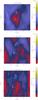 |
Fig. 3 Same as Fig. 2 for the MHD case. A weak magnetic field (1 μG) along the x-axis initially permeates the cloud. The filament remains much more coherent than in the hydrodynamical case. |
3. Simple preliminary numerical experiment
Before proceeding to the complex turbulent simulations, we present two simple numerical simulations that illustrate some of the conclusions that will be drawn later. It consists of a spherical cloud with a strong initial shear that therefore is prone to form a filament. More precisely, a spherical cloud of density 100 cm-3, temperature 100 K, and radius 0.5 pc was placed in the middle of the computational box and was embedded into a diffuse and warm medium of density 1 cm-3 and temperature 8000 K. The total box size is 20 pc. A transverse velocity gradient along the x-axis of 1.5 km s-1 pc-1 is initially imprinted through the box. Finally, a turbulent velocity field with a total rms dispersion of 5 km s-1 was superimposed in the box. The reason of superimposing this velocity field is to create self-consistent perturbations that disturb the forming filament. Two such simulations were performed, the first one was purely hydrodynamical while the second had a magnetic field of 1 μG, initially uniform and oriented along the x-axis and therefore perpendicular to the initial main component of the velocity field.
Figure 2 shows the column density for three snapshots of the hydrodynamical simulation. As is clear from the figure, the initially spherical cloud is stretched and evolves in a filament because of the shear. At the same time the nonlinear fluctuations induced by the surrounding medium perturb the cloud and very likely trigger the growth of various instabilities (such as the Kelvin-Helmholtz instability). The complex pattern displayed in the three snapshots is the result of the uniform shear and the turbulent fluctuations present in the surrounding medium. After 1.6 Myr the third panel shows that the filament is totally destroyed and broken up into many cloudlets. Note that the same simulations were repeated without turbulence superimposed initially. The filament in this case was more stable except that it broke in two parts.
Figure 3 shows the magnetized run. The early evolution of the dense cloud is initially similar. A filament forms due to the initial shear,. However, the late evolution is quite different. Although it is subject to strong fluctuations induced by the surrounding turbulent medium, the filament remains much more coherent. The reason for this is that initially the cloud is threated by a magnetic field, the pieces of fluid are connected to each other through the field lines. Moreover, the shear that tends to form the filament amplifies the magnetic field and it makes its influence stronger. Indeed, as the filament is getting stretched, the magnetic field is amplified along the y-axis and becomes largely parallel to the filament at the end of the simulation. This behavior agrees well with the studies of the development of the Kelvin-Helmholz instability that have been performed by various teams (e.g. Frank et al. 1996; Ryu et al. 2000). In these studies it has been found that even weak magnetic fields significantly modify the evolution of flows making it much more stable. Stronger fields, on the other hand, can completely stabilize the flow against this instability.
This simple experiment suggests a scenario for filament formation. The gas is compressed by converging motion but at the same time, the fluid particle possesses solenoidal modes inherited from the turbulent environment that tends to stretch it. Without a magnetic field, the pieces of fluid can easily move away from each other. When a magnetic field is present, the pieces of fluid are tightly connected to each other and the filament remains coherent for longer times.
4. Clump geometry
 |
Fig. 4 Column density, density, and velocity fields for one snapshot of the decaying turbulence experiment in the hydrodynamical case. |
 |
Fig. 5 Column density, density, and velocity fields for one snapshot of the decaying turbulence experiment in the MHD case. |
4.1. Qualitative description of decaying-turbulence simulations
Figures 4 and 5 show one snapshot at roughly one crossing time for the hydrodynamical and MHD cases. Column density (top panels) and density (bottom panels) together with velocity fields are shown. The column density was obtained by simple integration through the box, the density corresponds to the value in the z = 0 plane. As expected strong density contrast develop in both cases due to the large rms Mach numbers (about 3 initially to 1 in the WNM and 10 in the CNM). This is partly because of the 2-phase structure and partly because of the supersonic motions. The hydrodynamical and MHD cases present obvious differences however. Overall, the hydrodynamical case appears to be less filamentary than the MHD case, in which very high aspect ratio structures can be seen both in the column density and in the density. Some filamentary structures are also visible in the hydrodynamical case but they have lower aspect ratios. Moreover, as seen from the density and velocity fields, it is often the case that the velocity field is perpendicular to the elongated structure, suggesting that shocks are triggering them. Indeed, these structures are mainly sheets as shown below.
It is important to stress that at the beginning of our calculations which we recall started with uniform density and a velocity field constructed with ramdon phases, more high aspect ratio structures formed in the hydrodynamical phase. However, this is a transient phenomenon due to our somewhat arbitrary initial conditions. These clumps quickly re-expanded which led to the type of morphology seen in Fig. 4. This visual impression that the MHD simulations are more filamentary is clearly visible in various other works (Padoan et al. 2007; Hennebelle et al. 2008; Federrath & Klessen 2013).
Beyond this visual impression, it is important to carefully quantify the aspect ratio, which is the purpose of the following section.
4.2. Axis ratio of clumps
Here we attempt to quantify the clump aspect ratio using two different methods, the inertia matrix and the skeleton approach.
4.2.1. Aspect ratio calculated with the inertia matrix
 |
Fig. 6 Distribution of the aspect ratio, μ1/μ3 of the clumps (threshold 50 cm-3: upper panel and 200 cm-3: lower panel) in the hydrodynamical simulation at time t = 1.52 Myr (dotted lines) and t = 3.37 Myr (solid lines). |
 |
Fig. 7 Distribution of the aspect ratio, μ1/μ3 of the clumps in the MHD simulations. The bottom panel shows the distribution for the threshold n = 50 cm-3 and for 3 Mach numbers (solid line: ℳ = 10, dashed line: ℳ = 3, dotted line: ℳ = 1). The middle and top panels show the distribution at two different thresholds (middle: 50 cm-3, bottom: 200 cm-3) for the fiducial simulation (magnetized, ℳ = 10: solid line) at time 1.81 Myr and the high-resolution simulation at time 2.26 Myr (dotted line). |
As explained in Sect. 2.1.2, the inertia matrix was computed for all clumps and the aspect ratio was estimated as the quantity  , where I1 and I3 are the lowest and highest eigenvalues.
Figures 6 and 7 display the distribution of μ1/μ3 for the hydrodynamical and MHD simulations and for two thresholds, 50 (upper panels) and 200 cm-3 (lower panels for Fig. 6 and middle panel for Fig. 7). Clearly, the aspect ratios in the MHD simulations are lower by a factor of ≃1.5−2 than the aspect ratios in the hydrodynamical simulations. The threshold has only a modest influence on the resulting distribution.
The bottom panel of Fig. 7 shows that the Mach number has only a modest influence on this result. There are only small differences between ℳ = 10 and 3 runs (solid and dotted lines, respectively). The differences are more pronounced in the ℳ = 1 run but this could be due to the lack of statistics. The peak is possibly shifted toward slightly higher values, but stays below 0.2−0.3.
It is worth stressing that in all cases, most of the clumps have an aspect ratio lower than 0.3 and a good fraction of them have an aspect ratio lower than 0.2 and even 0.1. These last can be called filaments.
4.2.2. Triaxial clumps
 |
Fig. 8 Normalized bidimensional histogram displaying μ1/μ2 as a function of μ2/μ3. Top panel: hydrodynamical simulation at time 3.37 Myr. Bottom panel: MHD simulation at time 1.81 Myr. |
The aspect ratio of the highest over lowest eigenvalues only partially describes the clump geometry. It is necessary, for a more complete description, to investigate the distribution of the two ratios μ1/μ2 and μ2/μ3. Figure 8 displays the normalized bidimensional histograms for the hydrodynamical and MHD simulations using the density threshold of 200 cm-3. The two distributions present significant differences. The clumps from the hydrodynamical simulation tend to cover the μ1/μ2 − μ2/μ3 plane more uniformly. In particular, most of the points are located in a region with μ1/μ2 ≃ 0.2 − 0.6 and μ2/μ3 ≃ 0.3 − 0.8. These clumps can be described as ribbons or/and sheets. More quantitatively, we find that the fraction of clumps with μ2/μ3 between 0.2 and 0.8 and μ1/μ2 between 0.3 and 0.7 is 62%, of which about half have μ2/μ3 lower than 0.5. The number of clumps with μ2/μ3 lower than 0.3 and μ1/μ2 higher than 0.4 is only about 11%. In the MHD simulation, the values μ1/μ2 ≃ 0.5 and μ2/μ3 ≃ 0.25 are more typical. Such objects can be described as ribbons and/or filaments. The most important difference are the absence of spheroidal (μ1 ≃ μ2 ≃ μ3) clumps and the scarcity of sheet like clumps (μ1 ≪ μ2 ≃ μ3) in the MHD simulations. More quantitatively, the fraction of clumps with μ2/μ3 between 0.2 and 0.8 and μ1/μ2 between 0.3 and 0.7 is 52%, of which about 75% have μ2/μ3 lower than 0.5. The fraction of sheet-like or spheroidal-like objects (μ2/μ3 > 0.5) is therefore twice as low as in the hydrodynamical simulation. The number of filamentary clumps with μ2/μ3 lower than 0.3 and μ1/μ2 higher than 0.4 is about 30% which is three times more than in the hydrodynamical simulation.
Since sheet-like objects are produced by shocks, this clearly suggests that while shocks are important and numerous in the hydrodynamical simulations, they play a less important role in the MHD simulations. This is expected because the magnetic field certainly reduces their ability to compress the gas.
4.2.3. Aspect ratio calculated from skeleton approach
 |
Fig. 9 Same as Fig. 6 for the distribution of the aspect ratio, R/L of the clumps (threshold 50 cm-3: upper panel and 200 cm-3: lower panel) in the hydrodynamical simulation at time t = 1.52 Myr (dotted lines) and t = 3.37 Myr (solid lines). |
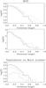 |
Fig. 10 Same as Fig. 7 for the distribution of the aspect ratio, R/L of the clumps. The bottom panel shows the distribution for the threshold n = 50 cm-3 and for 3 Mach numbers (solid line: ℳ = 10, dashed line: ℳ = 3, dotted line: ℳ = 1). The middle and top panels show the distribution at two different thresholds (middle: 50 cm-3, bottom: 200 cm-3) for the fiducial simulation (magnetized, ℳ = 10: solid line) at time 1.81 Myr and the high-resolution simulation at time 2.26 Myr (dotted line). |
To verify the trends inferred for the clump aspect ratio, we also calculated it using the skeleton approach and the definitions given in Sect. 2.2.1. The results for the two snapshots of the hydrodynamical and MHD simulations are presented in Figs. 9 and 10. As can be seen, the trends are very similar to what has been inferred from the inertia matrix and the distributions are generally quite comparable. In particular, the clumps tend to be more elongated in the MHD case than in the hydrodynamical case. One difference is the tail of few weakly elongated clumps (aspect ratio 0.5−1) however that is not apparent in the inertia matrix approach. This is likely due to the difference in the definition between the two methods.
The nice similarity of the distributions obtained with two completely different methods suggests that the two methods are indeed reliable however.
4.3. Length and thickness
We now turn to the study of the clump characteristic scales. The length is defined as the sum over all  within the clumps. This gives the sum of the length of all the branches which belong to the clumps and is therefore longer than the largest distance between two points in the clump. The thickness is defined as explained in Sect. 2.2.1, that is to say, as the mean distance between the clump cells and the clump local direction (defined by
  ).
).
4.3.1. Clump length
Figures 11 and 12 show the length distribution for the hydrodynamical and MHD simulations, respectively. The distributions are similar. They peak at about L ≃ 0.5 pc and decrease with size for lower values. This is very similar to the behavior of the clump mass spectra (e.g. Hennebelle & Audit 2007; Audit & Hennebelle 2010) and is a clear consequence of the numerical diffusion induced by the finite size of the mesh. The comparison between the fiducial simulation (top panel of Fig. 12) and the high-resolution run shows that these peaks tend to shift toward the smaller size although the extraction was performed at the same physical resolution as explained previously. At longer length, L, the distribution is close to a power law. This is more obvious for the ℳ = 10 simulations than for the ℳ = 3 and 1 cases (bottom panel of Fig. 12), probably because there are fewer clumps in these simulations and the statistics are poorer. Typically, we obtain  for the threshold 200 cm-3. The exponent is slightly shallower for the threshold 50 cm-3. Apart from the fact that turbulence generally tends to generate power laws, it is worth to understand the origin of this exponent better.
First of all, recalling that the mass spectra of clumps were found to be dN/dlog M ∝ M− αN + 1 with αN ≃ 1.8 by various authors (Hennebelle & Audit 2007; Heitsch et al. 2008; Dib et al. 2008; Audit & Hennebelle 2010; Inoue & Inutsuka 2012). This exponent is consistent with the value inferred by Hennebelle & Chabrier (2008) for turbulent clumps. Anticipating what we show in the next section, the thickness of the clumps, rc, stays roughly constant, i.e., is peaking toward a nearly constant value with a narrow distribution. But the mass of clumps is proportional to  , thus since rc is found to be roughly constant and the mean density in most of the clumps is on the order of the density threshold, one finds that the mass of the clumps is proportional to their length M ∝ L (we recall that L is the integrated length through all branches). Consequently, it is not surprising to find that dN/dlog L ∝ L-1, which is close enough to the clump mass spectrum.
4.3.2. Clump thickness
Figures 11 and 12 show the thickness distribution for the hydrodynamical and MHD simulations, respectively. The distributions of the hydrodynamical and MHD simulations at Mach 10 are similar. They peak at about ≃0.1 pc for both thresholds (with a small shift toward higher values for the lowest threshold 50 cm-3). This is similar to the behavior displayed by the length distribution, which also presents a peak, though shifted toward higher values. The higher resolution simulation (middle and top panels of Fig. 12) again show a systematic trend toward lower values. This is again consistent with the peak being a consequence of the numerical diffusion.
Unlike for the length distribution however, there is no power-law tail, instead, the whole distribution is a narrow peak (full width at half maximum of about 0.4). Thus we conclude that the thickness of the clumps (which also represents the thickness of filaments when only the very elongated ones are selected) is largely due to the finite resolution of the simulations. This in turns means that to physically describe the interstellar filaments down to their thickness, realistic dissipative processes should be consistently included (see the discussion section). We recall that the numerical algorithm used in this work is very similar to most methods implemented in other codes used in the study of the ISM and beyond. This conclusion is therefore not restricted to the present work only, but seemingly affects the simulations performed with solvers which do not explicitly treat the dissipative processes. Note that if instead of the mean radius, the distribution of all local radii is plotted, one finds that it typically extends to values about 3−4 times higher though most of the points are still close to a few grid points.
The thickness of the clumps presents some dependence on the Mach number, as shown in bottom panel of Fig. 12. However, changing the Mach number by a factor 10 leads to a shift of the size smaller than a factor 2. This contradicts the explanation that the interstellar filaments are entirely determined by shocks. A velocity perturbation at scale L has a typical amplitude V = V0(L/L0)0.5, as suggested by Larson relations (Larson 1981; Falgarone et al. 2009; Hennebelle & Falgarone 2012). The Rankine-Hugoniot conditions then lead to a density enhancement ρs/ρ ≃ (V/Cs)2 = (V0/Cs)2 × (L/L0) and to a thickness Ls/L = ρ/ρs = ℳ2. As can be seen, the thickness is expected to vary with ℳ2 which we do not observe in these simulations instead, a more shallow dependence on the Mach number is observed. This does not mean that compression has no effect at all. Indeed since these structures are denser than the surrounding medium, compression does occur. However, the very reason that these structures are elongated does not seem to be compression only.
5. Links between geometry, velocity, and forces
Next, we would like to understand why the clumps tend to have such a low aspect ratio, or in other words, why there are so many filaments in the simulations. So far, we have seen that the MHD simulations tend to be more filamentary than the hydrodynamical ones and that the aspect ratio does not strongly evolve with the Mach number. There is only a weak trend for it to decrease when ℳ increases (bottom panel of Fig. 7). These two facts do not straighforwardly agree with the earlier proposition that filaments are due to the collision of two shocked sheets (e.g. Padoan et al. 2001) and suggest that the process entails other aspects than mere compression. Indeed, in this scenario, one would expect high Mach number flows to be more filamentary, but because the magnetic field renders the collisions less supersonic, it is unclear why magnetized simulations would be more filamentary. On the other hand, the simple numerical experiment presented in Sect. 3 suggests that the filaments could simply be fluid particles that have been stretched by the turbulent motions. The most important difference with the shock scenario is that filaments are not born as elongated objects, but they become elongated as time elapses.
In this section we investigate whether the mechanism by which filaments form is indeed the stretch of the fluid particles induced by turbulence. It should be kept in mind that shocks or convergening motions, must play a role at some stage because the gas within the filaments must accumulate. The question is then how to estimate their respective influence.
5.1. Alignment between strain and filament axis
 |
Fig. 15 Same as Fig. 6 for the distribution of cosα (the angle between the main axis and the strain) in the clumps. |
 |
Fig. 16 Same as Fig. 7 for the distribution of cosα (the angle between the main axis and the strain) in the clumps. |
To investigate whether the filaments are indeed particle fluids that have been stretched by the turbulent motions, we studied the correlation between the eigenvector associated to the highest eigenvalue of the inertia matrix which we later call the filament axis, and the eigenvector of the highest eigenvalue of the strain tensor, which gives the direction along which the clumps are stretched. More precisely, we studied the distribution of cosα, where α is the angle between these two eigenvectors. Indeed, if the two eigenvectors tend to be aligned, this will be clear evidence that filaments are stretched by the velocity field.
Figures 15 and 16 show results for the two density thresholds. Clearly in all cases there are more clumps for which cosα is close to −1 or 1 than clumps for which cosα is close to 0. In other words, there is a trend for the filament axis and the strain to be aligned. This clearly shows that the primary cause of the existence of filaments, that is to say the existence of elongated clumps, is the stretching of the fluid particles induced by the turbulent motions. This does not imply that shocks may not be also forming filaments, in particular intersection between two shocked layers as it has been previously suggested. However, this cannot be the dominant mechanism because in such configurations, one would expect the filament axis and the strain to be randomly distributed.
A comparison between Figs. 15 and 16 also reveals that the trend is clearly more pronounced for MHD simulations than for hydrodynamical ones. For example, there are about 8−10 times more objects having | cosα | = 1 than objects with cosα = 0 in the MHD case. In the hydrodynamical case, this ratio is about 3 − 5. Again since the MHD simulation is more filamentary that the hydrodynamical one, this is not consistent with the dominant origin of filaments being due to shocks since magnetic field tends to reduce the effective Mach number. Finally, we see that in lower Mach simulations (dotted and dashed lines in the bottom panel in Fig. 16), this trends is also present albeit reduced.
5.2. Comparison between strain and divergence
The correlation between the strain and the filament axis suggests that strain is an important, if not the dominant reason for filaments within the ISM. However, the clumps are regions of high densities where the gas has been accumulated. Therefore it is important to understand the respective role of the compressive and the straining motions. For this purpose, we studied the ratio distribution of the divergence and the strain, rds, calculated as described in Sect. 2.2. This quantity allows us to directly estimate whether the structure is globally contracting or expanding and whether this global change of volume dominates or is dominated by the change of shape described by the strain.
Figure 17 shows results for the hydrodynamical simulation for the two thresholds (50 cm-3 upper panels and 200 cm-3 lower panels). The distribution of rds is pretty flat and extends between about − 1.2 and 1.2. It is roughly symmetrical with respect to 0, particularly for the lowest density threshold. This indicates that the contribution of compressive and solenoidal motions for the dynamics of the clumps is similar though most clumps have a mean strain larger than their divergence (but few clumps have a small rds). For our highest threshold, the number of expanding clumps is lower than the number of contracting clumps.
Figure 18 shows results for the MHD simulation. The general trends are qualitatively similar to the hydrodynamical simulations except for the important fact that the distributions are much less symmetrical with respect to zero. There are fewer expanding than contracting clumps. This suggests that the magnetic field tends to confine the clumps and hinders their reexpansion with the latter being generally dominant over the former.
5.3. Confinement by Lorentz force
 |
Fig. 19 Mean value of the Lorentz force radial component (see text) within the clumps (threshold 50 cm-3: upper panel and 200 cm-3: lower panel) for the high-resolution MHD simulation at time t = 2.26 Myr (dotted line) and the fiducial run at time 1.81 Myr (solid line). |
 |
Fig. 20 Same as Fig. 19 for the mean value of the pressure force radial component (see text) within the clumps. |
To verify that the Lorentz force is indeed reducing the clump expansion, we computed the mean component of the Lorentz force in the direction perpendicular to the local direction of the clumps. To accomplish this, given a cell center M, we first computed the position of M′ defined by  , that is to say, M is projected onto the local axis in M′ (
 is defined as explicited in Sect. 2.2.1). The component of the force perpendicular to the local direction of the clump () is thus simply F(M).MM′/ | MM′ |. The total contribution is thus obtained by summing over the whole structure
  (1)The result is displayed in Fig. 19 for the two density thresholds. As can be seen, there are structures that the Lorentz force tends globally to confine (integrated component is negative) and structures that it tends to expand. However, it is clearly skewed toward the negative values and in most cases the Lorentz force tends to confine the structure and maintain the coherence of the clumps. More quantitatively, we find that depending on the run parameters and thresholds, the fraction of clumps for which the integrated component of the Lorentz force is negative is between 55 and 65%.
For comparison, it is interesting to investigate the effect of the pressure force. The corresponding distribution is plotted in Fig. 20. As expected, the pressure force tends almost always to expand the structure. We also see from the amplitude that the Lorentz force largely dominates over the pressure force.
These results agree well with the results inferred from the divergence of strain ratio, rds and also with the simple numerical experiment presented in Sect. 3. The magnetic force tends to prevent the clump re-expansion because the magnetic field lines permeate through the clumps and connect the fluid particles.
6. Discussion
The role played by two important processes, namely non-ideal MHD effects and gravity, has not been included or investigated in this work and requires at least some discussions.
6.1. The role of dissipative processes
Although our simulations seem to roughly agree with the Herschel observations about the constancy of the filament inferred by Arzoumanian et al. (2011), it is important to keep in mind that this thickness is most likely set up in the present simulations (and in any similar simulation) by the numerical diffusion, which operates at the scale of a few computing cells (here about 0.05 pc for the fiducial run). Therefore, although encouraging, this resemblance must be taken with the greatest care at this stage. Moreover, our filaments were selected using a density threshold that is also different from that of Arzoumanian et al. (2011).
Nevertheless, the conclusion that the thickness of the filaments, at least in the way we defined them, is set up by a dissipative process is intriguing and leads to the obvious question of which dissipative mechanism could actually produce a scale similar to a size of 0.1 pc. The only known dissipative mechanism in the interstellar medium, that leads to comparable scales is the ion-neutral friction as investigated by Kulsrud & Pearce (1969).
We recall that when ion-neutral friction is taken into consideration, the induction equation can be written as  (2)where γad is the ion-neutral friction coefficient, whose value is about γad ≃ 3.5 × 10¹³ g-1 s-1 (e.g. Shu et al. 1987).
Although the right-hand side has not the standard form of a diffusion, it is a second order term that dissipates mechanical energy into heat. We can easily compute a magnetic Reynolds number associated to this equation as  (3)where ν = B2/(4πγadρρi). As is done in standard approach of turbulence, we assume that the energy flux, ϵ = ρV(l)3/l, is constant through the scales. Thus we can write
  (4)Estimating ϵ at the integral scale, L0, we obtain
  (5)The smallest scale that can be reached in a turbulent cascade is typically obtained when the Reynolds number is equal to about 1. This leads for ldiss, the dissipation length, the following expression:
  (6)The impact of non-ideal MHD processes on the density field can be clearly seen in the simulations performed by Downes & O’Sullivan (2009, 2011). These authors have run similations of molecular clouds at a scale of 0.2 pc. Figure 1 of these two papers display the density field in the ideal MHD case and in the non-ideal MHD one. Clearly, many small-scale filaments are seen in the ideal MHD simulation, which evidently are very close to the numerical resolution. This is very different from what is seen in the non-ideal MHD simulations, in which only large scale-structures (bigger that the cell size) are produced. Interestingly, the large-scale patern is unchanged, but the small scales are completely differents. These simulations demonstrate that indeed non-ideal MHD processes have a very strong impact on the clump structure.
To estimate the dissipation length we used typical values for the diffuse interstellar medium. The values of V0, ρ0 = mpn0 and L0 are linked through the Larson relations (Larson 1981). We chose as fiducial values V0 = 2.5 km s-1, ρ0 = 100 cm-3 and L0 = 10 pc. Typical magnetic fields are about 5 μG in the diffuse gas and 10−20 μG in the molecular gas for densities of a few 103 cm-3. The ionization is also important and varies significantly.
In the molecular gas the ionization is about 10-6 − 10-7 (Le Petit et al. 2006; Bergin & Tafalla 2007) and the ion density ρi can be approximated as  , where C = 3 × 10-16 cm−3/2 g1/2. Using this expression, a density of 103 cm-3 and a magnetic field of 20 μG, we obtain ldiss ≃ 0.2 pc, which is entirely reasonable. Note that assuming that the magnetic field increases as
  (e.g. Crutcher 1999), we find that the density dependence is extremely shallow, seemingly suggesting that this scale could indeed be representative of a broad range of conditions. These numbers as well as the analysis are similar to the results presented in McKee et al. (2010).
In the diffuse gas, which has a density of only a few 100 cm-3, the ionization is about 10-4 − 10-5 (e.g. Wolfire et al. 2003), which leads for a density of 200 cm-3 and a magnetization of 5 μG to ldiss ≃ 3 × 10⁻³ − 2 × 10⁻² pc, that is to say, much lower values.
It is important to stress that these numbers remain indicative only at this stage and should not be directly interpreted as the sizes of the structures, which can certainly be different by a factor of a few. Nevertheless, a clear consequence of these estimates is that the filaments are probably much thinner in the weakly shielded gas (Av < 1), in particular in the HI and at the periphery of molecular clouds.
6.2. Influence of gravity
Gravity can also play an important role in the formation of massive filaments. Indeed, gravity is well known to amplify initial anisotropies (Lin et al. 1965) and has been found in various studies to play an important role in triggering the formation of self-gravitating filaments (Hartmann & Burkert 2007; Peretto et al. 2007). Indeed, in these studies gravity acts to amplify the initial elongation of a clump that could have been induced by turbulence.
It is therefore likely that gravity can play a significant role in the formation of the most massive filaments and maybe even for setting the width of the marginally self-gravitating ones, as recently advocated by Fischera & Martin (2012; see also Heitsch 2013).
The nature of this elongation is quite different from what has been studied here. It is a selective contraction along two directions instead of a stretching along one direction. We stress, however, that gravity is self-consistently included in the collision-flow calculations presented in Appendix B, and that as discussed there the results are very similar to what has been found for the more diffuse ISM studied in the paper. Thus it is seems that except probably for very dense filaments (e.g. integral-shaped Orion or DR21 filaments), gravity does not modify the picture very significantly.
7. Conclusion
We have performed a series of numerical simulations to study the formation of clumps in the turbulent ISM, paying particular attention to the reason that causes the elongation. We ran both hydrodynamical and MHD simulations and varied the Mach number. To verify the robustness of our results, we used two different setups, decaying turbulence and colliding-flows. To quantify the structure properties, we first extracted the clumps using a simple clipping algorithm. We then computed and diagonalized the inertia matrix and the strain tensor. We also developed a skeleton-like approach, which allowed to infer the mean thickness and to compute whether forces tend to expand or confine the structures. We found that in all simulations most of the clumps are significantly elongated and the main axis of the structure tends to be aligned with the strain, particularly in MHD simulations. The proportion of filamentary objects is higher in the MHD simulations than in the hydrodynamical ones, in which a significant fraction of the clumps are sheets rather than filaments. While the pressure force tends to expand the clumps as expected, the Lorentz force tends on average to confine them, allowing the filaments to remain longer. In all simulations, irrespective of the magnetic intensity and Mach number, we found that the thickness of the clumps, that is to say the mean thickness of all the clump branches, is always close to a few computing cells seemingly suggesting that in the ISM dissipative processes are responsible of setting its value. Performing simple orders of magnitude, we find that the ion-neutral friction in regions of sufficient extinction leads to values that are close to what has recently been inferred from Herschel observations (Arzoumanian et al. 2011). In unshielded regions such as HI or in the outskirts of molecular clouds where the ionization is higher, this would imply that the filament thickness should be at least ten times lower.
Online material
Appendix A: Results of decaying turbulence with a magnetic field tilted with respect to the mesh
Because we found in this paper that the clumps are more filamentary in magnetized flows, it is important to verify that no obvious numerical artifact is producing this effect. We therefore repeated one of the runs (decaying turbulence with 5 μG and one level of AMR) with a magnetic field initially tilted to 45° with respect to the mesh. Figures A.1 and A.2 show the bidimensional distribution μ1/μ2 vs. μ2/μ3 and the histogram of cos(α), the cosine of the angle between the filament axis and the strain, respectivelly. As can be seen, they are very similar to the corresponding results shown for the untilted case.
 |
Fig. A.1 Normalized bidimensional histogram displaying μ1/μ2 as a function of μ2/μ3 for the decaying turbulence simulation with inclined magnetic field at time 1.32 Myr. |
 |
Fig. A.2 Distribution of cosα (the angle between the main axis and the strain) in the clumps for the decaying turbulence simulation with inclined magnetic field at time 1.32 Myr. |
Appendix B: Results of colliding flow simulations
Here we present the results obtained for the colliding-flow simulations. These simulations are described in Sect. 2.3.2. The purpose of this appendix is to demonstrate that the results obtained in the paper are not a consequence of a particular choice of initial and boundary conditions. We used time steps that represent a similar evolution. For the four runs, significant masses of gas (typically 104 M⊙ of gas denser than 100 cm-3) were accumulated, and at several places, collapse has proceeded or is still proceeding. We restrict our attention to the most important quantities that were studied namely the clump aspect ratio computed using the inertia matrix and the skeleton-like approach, the length and thickness of the clumps, the cosine of the angle between the clump axis, and the strain and the divergence over strain ratio. In the six plots the solid line represents the high-resolution intermediate magnetization run, the dotted line is the standard resolution intermediate magnetization one, the dashed line represents the highly magnetized run while the dot-dashed line displays the hydrodynamical simulation.
 |
Fig. B.1 Distribution of aspect ratio, μ3/μ1 of the clumps (threshold 500 cm-3). Solid line: high-resolution intermediate magnetization run at time 12.94 Myr. Dotted line: standard resolution intermediate magnetization run at time 16.82 Myr. Dashed line: highly magnetized run at time 18 Myr. Dot-dashed line: hydrodynamical run at time 15.1 Myr. |
 |
Fig. B.2 Same as Fig. B.1 for the distribution of aspect ratio, R/L of the clumps (threshold 500 cm-3). |
Figures B.1 and B.2 show very similar trends with Figs. 6, 7, 9 and 10. In particular, in the hydrodynamical simulation the clumps have larger aspect ratios than in the MHD simulations.
The length and the thickness of the clumps are very similar to what has been inferred in the decaying simulations. The peaks are also located at the same position of about 0.5 pc for the length and 0.1 pc for the thickness.
In Fig. B.5 the trends of the filament axis and the strain to be preferentially aligned is also clear. As for the decaying turbulence simulations, it is more pronounced for the magnetized than for the hydrodynamical runs.
Figure B.6 is also very similar to the trends inferred in Figs. 17 and 18 that were discussed previously.
 |
Fig. B.5 Same as Fig. B.1 for the distribution of cosα (the angle between the main axis and the strain) in the clumps. |
Acknowledgments
I thank the anonymous referee for insightful comments. I thank Pierre Lesaffre, Philippe André, and Doris Arzoumanian for many related and inspiring discussions. This work was granted access to HPC resources of CINES under the allocation x2009042036 made by GENCI (Grand Equipement National de Calcul Intensif). P.H. acknowledge the finantial support of the Agence National pour la Recherche through the COSMIS project. This research has received funding from the European Research Council under the European Community’s Seventh Framework Programme (FP7/2007-2013 Grant Agreement No. 306483).
References
- André, P., Men’shchikov, A., Bontemps, S., et al. 2010, A&A, 518, L102 [NASA ADS] [CrossRef] [EDP Sciences] [Google Scholar]
- Arzoumanian, D., André, Ph., Didelon, P., et al. 2011, A&A, 529, L6 [Google Scholar]
- Audit, E., & Hennebelle, P. 2005, A&A, 433, 1 [NASA ADS] [CrossRef] [EDP Sciences] [Google Scholar]
- Bally, J., Lanber, W., Stark, A., & Wilson, R. 1987, ApJ, 312, L45 [NASA ADS] [CrossRef] [Google Scholar]
- Banerjee, R., Vázquez-Semadeni, E., Hennebelle, P., & Klessen, R. 2009, MNRAS, 398, 1082 [NASA ADS] [CrossRef] [Google Scholar]
- Bergin, E., & Tafalla, M. 2007, ARA&A, 35, 179 [Google Scholar]
- Crutcher, R. 1999, ApJ, 520, 706 [NASA ADS] [CrossRef] [Google Scholar]
- de Avillez, M., & Breitschwerdt, D. 2005, A&A, 436, 585 [NASA ADS] [CrossRef] [EDP Sciences] [Google Scholar]
- Dib, S., Brandenburg, A., Kim, J., Gopinathan, M., & André, P. 2008, ApJ, 678, L105 [NASA ADS] [CrossRef] [Google Scholar]
- Downes, T., & O’Sullivan, S. 2009, ApJ, 701, 1258 [NASA ADS] [CrossRef] [Google Scholar]
- Downes, T., & O’Sullivan, S. 2011, ApJ, 730, 12, [NASA ADS] [CrossRef] [Google Scholar]
- Falgarone, E., Pety, J., & Hily-Blant, P. 2009, A&A, 507, 355 [NASA ADS] [CrossRef] [EDP Sciences] [Google Scholar]
- Federrath, C., & Klessen, R. 2013, ApJ, 763, 51 [NASA ADS] [CrossRef] [Google Scholar]
- Fischera, J., & Martin, P. 2012, A&A, 542, A77 [NASA ADS] [CrossRef] [EDP Sciences] [Google Scholar]
- Frank, A., Jones, T., Ryu, D., & Gaalaas, J. 1996, ApJ, 460, 777 [NASA ADS] [CrossRef] [Google Scholar]
- Fromang, S., Hennebelle, P., & Teyssier, R. 2006, A&A, 457, 371 [NASA ADS] [CrossRef] [EDP Sciences] [Google Scholar]
- Hartmann, L., & Burkert, A. 2007, ApJ, 654, 988 [NASA ADS] [CrossRef] [Google Scholar]
- Heitsch, F. 2013, ApJ, 769, 115 [NASA ADS] [CrossRef] [Google Scholar]
- Heitsch, F., Burkert, A., Hartmann, L., Slyz, A., & Devriendt, J. 2005, ApJ, 633, 113 [NASA ADS] [CrossRef] [Google Scholar]
- Heitsch, F., Hartmann, L., Slyz, A., Devriendt, J., & Burkert, A. 2008, ApJ, 674, 316 [NASA ADS] [CrossRef] [Google Scholar]
- Hennebelle, P., & Audit, E. 2007, A&A, 465, 431 [NASA ADS] [CrossRef] [EDP Sciences] [Google Scholar]
- Hennebelle, P., & Chabrier, G. 2008, ApJ, 684, 395 [NASA ADS] [CrossRef] [Google Scholar]
- Hennebelle, P., & Falgarone, E. 2012, A&ARv, 20, 55 [NASA ADS] [CrossRef] [Google Scholar]
- Hennebelle, P., Banerjee, R., Vázquez-Semadeni, E., Klessen, R., & Audit, E. 2008, A&A, 486, L43 [NASA ADS] [CrossRef] [EDP Sciences] [Google Scholar]
- Inoue, T., & Inutsuka, S.-I. 2012, ApJ, 759, 35 [NASA ADS] [CrossRef] [Google Scholar]
- Inoue, T., Yamazaki, R., & Inutsuka, S.-i. 2009, ApJ, 695, 825 [NASA ADS] [CrossRef] [Google Scholar]
- Joung, R., & Mac Low, M.-M. 2006, ApJ, 653, 1266 [NASA ADS] [CrossRef] [Google Scholar]
- Kulsrud, R., & Pearce, W. 1969, ApJ, 156, 445 [Google Scholar]
- Larson, R. 1981, MNRAS, 194, 809 [CrossRef] [Google Scholar]
- Le Petit, F., Nehmé, C., Le Bourlot, J., & Roueff, E. 2006, ApJS, 164, 506 [NASA ADS] [CrossRef] [EDP Sciences] [Google Scholar]
- Low, F., Young, E., Beintema, D., et al. 1984, ApJ, 278, L19 [NASA ADS] [CrossRef] [Google Scholar]
- McKee, C., Li, P.-S., & Klein, R. 2010, ApJ, 720, 1612 [NASA ADS] [CrossRef] [Google Scholar]
- Miville-Deschênes, M.-A., Martin, P., & Abergel, A. 2010, A&A, 518, L104 [NASA ADS] [CrossRef] [EDP Sciences] [Google Scholar]
- Miyoshi, T., & Kusano, K. 2005, JCoPh, 208, 315 [Google Scholar]
- Nagai, T., Inutsuka, S.-I., & Miyama, S. 1998, ApJ, 506, 306 [NASA ADS] [CrossRef] [Google Scholar]
- Nakamura, F., & Li, Z.-Y. 2008, ApJ, 687, 354 [NASA ADS] [CrossRef] [Google Scholar]
- Padoan, P., Juvela, M., Goodman, A., & Nordlund, A. 2001, ApJ, 553, 227 [NASA ADS] [CrossRef] [Google Scholar]
- Padoan, P., Nordlund, A., Kritsuk, A., Norman, M., & Li, P.-S. 2007, ApJ, 661, 972 [NASA ADS] [CrossRef] [Google Scholar]
- Peretto, N., Hennebelle, P., & André, P. 2007, A&A, 464, 983 [NASA ADS] [CrossRef] [EDP Sciences] [Google Scholar]
- Price, D., & Bate, M. 2008, MNRAS, 385, 1820 [NASA ADS] [CrossRef] [Google Scholar]
- Ryu, D., Jones, T., & Frank, A. 2000, ApJ, 545, 475 [NASA ADS] [CrossRef] [Google Scholar]
- Seifreid, D., Schmidt, W., & Niemeyer, J. 2011, A&A, 526, A14 [NASA ADS] [CrossRef] [EDP Sciences] [Google Scholar]
- Shu, F. H., Adams, F. C., & Lizano, S. 1987, ARA&A, 25, 23 [Google Scholar]
- Sousbie, T., Colombi, S., & Pichon, C. 2009, MNRAS, 393, 457 [NASA ADS] [CrossRef] [Google Scholar]
- Teyssier, R. 2002, A&A, 385, 337 [NASA ADS] [CrossRef] [EDP Sciences] [Google Scholar]
- Ungerechts, H., & Thaddeus, P. 1987, ApJS, 63, 645 [NASA ADS] [CrossRef] [Google Scholar]
- Vázquez-Semadeni, E., Banerjee, R., Gómez, G., et al. 2011, MNRAS, 414, 2511 [NASA ADS] [CrossRef] [Google Scholar]
- Ward-Thompson, D., Kirk, J., & André, P. 2010, A&A, 518, L92 [NASA ADS] [CrossRef] [EDP Sciences] [Google Scholar]
- Wolfire, M. G., Hollenbach, D., & McKee, C. F. 1995, ApJ, 443, 152 [Google Scholar]
- Wolfire, M. G., Hollenbach, D., & McKee, C. F. 2003, ApJ, 587, 278 [NASA ADS] [CrossRef] [Google Scholar]
All Figures
|
Fig. 1 Column density and velocity field for one of the clumps formed in the MHD simulations. The white points represent the local mass center Gij and constitute the skeleton of the clump. The upward pointing arrow represents the filament main axis as computed with the inertia matrix. The downward pointing arrow represents the main direction of the strain as computed with the strain tensor. |
| In the text | |
|
Fig. 2 Formation of a filament from a spherical cloud in the presence of shear, vy(x). The column density for three snapshots is displayed. Hydrodynamical case. The filament quickly fragments in many cloudlets. |
| In the text | |
|
Fig. 3 Same as Fig. 2 for the MHD case. A weak magnetic field (1 μG) along the x-axis initially permeates the cloud. The filament remains much more coherent than in the hydrodynamical case. |
| In the text | |
|
Fig. 4 Column density, density, and velocity fields for one snapshot of the decaying turbulence experiment in the hydrodynamical case. |
| In the text | |
|
Fig. 5 Column density, density, and velocity fields for one snapshot of the decaying turbulence experiment in the MHD case. |
| In the text | |
|
Fig. 6 Distribution of the aspect ratio, μ1/μ3 of the clumps (threshold 50 cm-3: upper panel and 200 cm-3: lower panel) in the hydrodynamical simulation at time t = 1.52 Myr (dotted lines) and t = 3.37 Myr (solid lines). |
| In the text | |
|
Fig. 7 Distribution of the aspect ratio, μ1/μ3 of the clumps in the MHD simulations. The bottom panel shows the distribution for the threshold n = 50 cm-3 and for 3 Mach numbers (solid line: ℳ = 10, dashed line: ℳ = 3, dotted line: ℳ = 1). The middle and top panels show the distribution at two different thresholds (middle: 50 cm-3, bottom: 200 cm-3) for the fiducial simulation (magnetized, ℳ = 10: solid line) at time 1.81 Myr and the high-resolution simulation at time 2.26 Myr (dotted line). |
| In the text | |
|
Fig. 8 Normalized bidimensional histogram displaying μ1/μ2 as a function of μ2/μ3. Top panel: hydrodynamical simulation at time 3.37 Myr. Bottom panel: MHD simulation at time 1.81 Myr. |
| In the text | |
|
Fig. 9 Same as Fig. 6 for the distribution of the aspect ratio, R/L of the clumps (threshold 50 cm-3: upper panel and 200 cm-3: lower panel) in the hydrodynamical simulation at time t = 1.52 Myr (dotted lines) and t = 3.37 Myr (solid lines). |
| In the text | |
|
Fig. 10 Same as Fig. 7 for the distribution of the aspect ratio, R/L of the clumps. The bottom panel shows the distribution for the threshold n = 50 cm-3 and for 3 Mach numbers (solid line: ℳ = 10, dashed line: ℳ = 3, dotted line: ℳ = 1). The middle and top panels show the distribution at two different thresholds (middle: 50 cm-3, bottom: 200 cm-3) for the fiducial simulation (magnetized, ℳ = 10: solid line) at time 1.81 Myr and the high-resolution simulation at time 2.26 Myr (dotted line). |
| In the text | |
 |
Fig. 11 Same as Fig. 6 for the length distribution of the clumps. |
| In the text | |
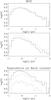 |
Fig. 12 Same as Fig. 7 for the length distribution of the clumps. |
| In the text | |
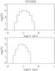 |
Fig. 13 Same as Fig. 6 for the thickness distribution of the clumps. |
| In the text | |
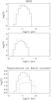 |
Fig. 14 Same as Fig. 7 for the thickness distribution of the clumps. |
| In the text | |
|
Fig. 15 Same as Fig. 6 for the distribution of cosα (the angle between the main axis and the strain) in the clumps. |
| In the text | |
|
Fig. 16 Same as Fig. 7 for the distribution of cosα (the angle between the main axis and the strain) in the clumps. |
| In the text | |
 |
Fig. 17 Same as Fig. 6 for the ratio distribution of the divergence and strain in the clumps. |
| In the text | |
 |
Fig. 18 Same as Fig. 7 for the ratio distribution of the divergence and strain in the clumps. |
| In the text | |
|
Fig. 19 Mean value of the Lorentz force radial component (see text) within the clumps (threshold 50 cm-3: upper panel and 200 cm-3: lower panel) for the high-resolution MHD simulation at time t = 2.26 Myr (dotted line) and the fiducial run at time 1.81 Myr (solid line). |
| In the text | |
|
Fig. 20 Same as Fig. 19 for the mean value of the pressure force radial component (see text) within the clumps. |
| In the text | |
|
Fig. A.1 Normalized bidimensional histogram displaying μ1/μ2 as a function of μ2/μ3 for the decaying turbulence simulation with inclined magnetic field at time 1.32 Myr. |
| In the text | |
|
Fig. A.2 Distribution of cosα (the angle between the main axis and the strain) in the clumps for the decaying turbulence simulation with inclined magnetic field at time 1.32 Myr. |
| In the text | |
|
Fig. B.1 Distribution of aspect ratio, μ3/μ1 of the clumps (threshold 500 cm-3). Solid line: high-resolution intermediate magnetization run at time 12.94 Myr. Dotted line: standard resolution intermediate magnetization run at time 16.82 Myr. Dashed line: highly magnetized run at time 18 Myr. Dot-dashed line: hydrodynamical run at time 15.1 Myr. |
| In the text | |
|
Fig. B.2 Same as Fig. B.1 for the distribution of aspect ratio, R/L of the clumps (threshold 500 cm-3). |
| In the text | |
 |
Fig. B.3 Same as Fig. B.1 for the length distribution of the clumps. |
| In the text | |
 |
Fig. B.4 Same as Fig. B.1 for the thickness distribution of the clumps. |
| In the text | |
|
Fig. B.5 Same as Fig. B.1 for the distribution of cosα (the angle between the main axis and the strain) in the clumps. |
| In the text | |
 |
Fig. B.6 Same as Fig. B.1 for the ratio distribution of the divergence and strain in the clumps. |
| In the text | |
Current usage metrics show cumulative count of Article Views (full-text article views including HTML views, PDF and ePub downloads, according to the available data) and Abstracts Views on Vision4Press platform.
Data correspond to usage on the plateform after 2015. The current usage metrics is available 48-96 hours after online publication and is updated daily on week days.
Initial download of the metrics may take a while.