| Issue |
A&A
Volume 556, August 2013
|
|
|---|---|---|
| Article Number | A68 | |
| Number of page(s) | 23 | |
| Section | Extragalactic astronomy | |
| DOI | https://doi.org/10.1051/0004-6361/201220969 | |
| Published online | 30 July 2013 | |
He II emitters in the VIMOS VLT Deep Survey: Population III star formation or peculiar stellar populations in galaxies at 2 < z < 4.6?⋆,⋆⋆
1
Aix Marseille Université, CNRS, LAM (Laboratoire d’Astrophysique de
Marseille) UMR 7326,
13388
Marseille,
France
e-mail:
paolo.cassata@oamp.fr
2
UPMC–CNRS, UMR 7095, Institut d’Astrophysique de
Paris, 75014
Paris,
France
3
Institut de Recherche en Astrophysique et Planétologie, CNRS,
Université de Toulouse, 14 avenue
E. Belin, 31400
Toulouse,
France
4
INAF–Osservatorio Astronomico di Bologna, via Ranzani
1, 40127
Bologna,
Italy
5
IASF–INAF, via Bassini 15, 20133
Milano,
Italy
6
Astronomical Observatory of the Jagiellonian
University, ul. Orla
171, 30-244
Kraków,
Poland
7
National Centre for Nuclear Research, ul. Hoża 69,
00-681
Warsaw,
Poland
8
INAF IASFBO, via P. Gobetti 101, 40129
Bologna,
Italy
Received: 20 December 2012
Accepted: 22 April 2013
Aims. The aim of this work is to identify He II emitters at 2 < z < 4.6 and to constrain the source of the hard ionizing continuum that powers the He II emission.
Methods. We assembled a sample of 277 galaxies with a highly reliable spectroscopic redshift at 2 < z < 4.6 from the VIMOS-VLT Deep Survey (VVDS) Deep and Ultra-Deep data, and we identified 39 He II λ1640 emitters. We studied their spectral properties, measuring the fluxes, equivalent widths (EW), and full width at half maximum (FWHM) for most relevant lines, including He II λ1640, Lyα line, Si II λ1527, and C IV λ1549.
Results. About 10% of galaxies at z ~ 3 and iAB ≤ 24.75 show He II in emission, with rest frame equivalent widths EW0 ~ 1–7 Å, equally distributed between galaxies with Lyα in emission or in absorption. We find 11 (3.9% of the global population) reliable He II emitters with unresolved He II lines (FWHM0 < 1200 km s-1), 13 (4.6% of the global population) reliable emitters with broad He II emission (FWHM0 > 1200 km s-1), 3 active galactic nuclei (AGN), and an additional 12 possible He II emitters. The properties of the individual broad emitters are in agreement with expectations from a Wolf-Rayet (W-R) model. Instead, the properties of the narrow emitters are not compatible with this model, nor with predictions of gravitational cooling radiation produced by gas accretion, unless this is severely underestimated by current models by more than two orders of magnitude. Rather, we find that the EW of the narrow He II line emitters are in agreement with expectations for a Population III (PopIII) star formation, if the episode of star formation is continuous, and we calculate that a PopIII star formation rate (SFR) of 0.1–10 M⊙ yr-1 alone is enough to sustain the observed He II flux.
Conclusions. We conclude that narrow He II emitters are powered either by the ionizing flux from a stellar population rare at z ~ 0 but much more common at z ~ 3, or by PopIII star formation. As proposed by Tornatore and collaborators, incomplete interstellar medium mixing may leave some small pockets of pristine gas at the periphery of galaxies from which PopIII may form, even down to z ~ 2 or lower. If this interpretation is correct, we measure at z ~ 3 a star formation rate density in PopIII stars of 10-6 M⊙ yr-1 Mpc-3, higher than, but qualitatively comparable to the value predicted by Tornatore and collaborators.
Key words: galaxies: evolution / galaxies: formation / galaxies: star formation / stars: Population III / galaxies: stellar content / stars: Wolf-Rayet
Figures 2–8, and 12 are available in electronic form at http://www.aanda.org
Based on data obtained with the European Southern Observatory Very Large Telescope, Paranal, Chile, under Large Programs 070.A-9007 and 177.A-0837. Based on observations obtained with MegaPrime/MegaCam, a joint project of CFHT and CEA/DAPNIA, at the Canada-France-Hawaii Telescope (CFHT) which is operated by the National Research Council (NRC) of Canada, the Institut National des Sciences de l’Univers of the Centre National de la Recherche Scientifique (CNRS) of France, and the University of Hawaii. This work is based in part on data products produced at TERAPIX and the Canadian Astronomy Data Centre as part of the Canada-France-Hawaii Telescope Legacy Survey, a collaborative project of NRC and CNRS.
© ESO, 2013
1. Introduction
Understanding the early phases of star formation in the Universe is a major topic of recent astrophysical investigation. In particular, despite the growing size of galaxy samples at z > 5–8, selected either through the Lyman-break technique (e.g., Bouwens et al. 2007, 2008, 2010; McLure et al. 2011) or via strong Lyα emission detected in narrow band filters (Hu et al. 2004; Tapken et al. 2006; Murayama et al. 2007; Hibon et al. 2010, 2012), some of which have spectroscopic confirmation (Vanzella et al. 2009; Capak et al. 2011; Curtis-Lake et al. 2012; Schenker et al. 2012), the population responsible for the reionization of the Universe at this epoch has not been identified yet. In this respect, zero metallicity stars and/or proto-galaxies, which should be the first structures formed in the life of the Universe and whose role in ionizing the Universe is predicted to be very important, have not been identified yet. The first population of stars formed from the pristine gas during the reionization is the so-called Population III (PopIII). This population is predicted to be of extremely low metallicity and to produce strong UV ionizing continuum (Tumlinson & Shull 2000; Schaerer 2002). No evidence for PopIII stars has been found so far. Moreover, despite the high efficiency of the cold mode gas accretion in cosmological simulation (Keres et al. 2005; Dekel et al. 2009), which may be enough to sustain the observed rapid increase of the star formation rate density (SFRD) of the Universe between z ~ 8 and z ~ 2, scarce evidence for gas infalling onto an overdensity has been reported so far. Steidel et al. (2010) found only partial evidence of inflow around galaxies at z ~ 2; Cresci et al. (2010) claimed that the inverted metallicity gradient observed in z ~ 3 galaxies could be due to cold flows; Giavalisco et al. (2011) detected cold gas around z ~ 1.6 galaxies that is possibly infalling into an overdensity.
Coincidently, the footprint of both PopIII star formation and gas cooling during gravitational accretion is the presence of Lyαλ 1216 and He II λ 1640 emission lines in the spectra of the sources. Dual Lyαλ 1216 and He II λ 1640 emitters have been proposed by various authors as candidates hosting PopIII star formation (Tumlinson et al. 2001; Schaerer 2003; Raiter et al. 2010). In PopIII star formation regions, where an extreme top-heavy initial mass function (IMF) is expected, very massive stars with high effective temperatures are formed. These stars, unlike normal PopII and PopI stars, produce photons shorter by λ = 228 Å that can ionize He+. In a region with primeval composition and in the absence of other metals, the H and He lines become the dominant line coolant for the gas, and thus the gas emits strong Lyα + He II emission. On the other hand, Fardal et al. (2001) showed that the pristine gas recently accreted onto an overdensity cools down and emits hydrogen or helium line radiation; Yang et al. (2006) claimed that dual Lyαλ 1216 and He II λ 1640 can be used to trace the infall of pristine gas onto an overdensity. If the accretion mode is cold, as predicted by many theoretical studies (Fardal et al. 2001; Keres et al. 2005), the gas temperature is below the halo virial temperature, reaching T ~ 105 K; if the gas is pristine (zero metallicity), H and He lines are the most efficient gas coolants, and thus Lyαλ 1216 and He II λ 1640 emission is produced.
Strong Lyα +He II emission lines are commonly found in other astrophysical objects, such as Wolf-Rayet (W-R) stars, AGN, and supernovae driven winds. However, several diagnostics can be used to distinguish cooling radiation and PopIII star formation from these other mechanisms: AGN, W-R stars and emitters powered by supernovae driven winds typically show other emission lines in their spectra, such as C III and C IV (Reuland et al. 2007; Leitherer et al. 1996; Allen et al. 2008). Moreover, W-R stars are associated with strong winds, and thus produce broad emission lines (a few 1000 km s-1, Schaerer 2003). Brinchmann et al. (2008a) showed that the broad He II emission detected in the composite spectrum of z ~ 3 galaxies by Shapley et al. (2003) can indeed be reproduced by W-R models. In W-R galaxies, or young star clusters with heavy star formation, He II emission may be observed in either a W-R stellar mode and broadened by the W-R winds, or in a nebular narrow-line mode as the strong UV emission from these stars photoionizes the surronding medium (Kudritzki 2002). Nebular He II emission also appears in some star forming regions in which the source of ionisation is not clearly identified as W-R or O stars, but this is a rare event in the local universe (Kehrig et al. 2011).
Unfortunately, no direct diagnostics can be used to distinguish between some extreme PopI populations, PopIII, or cooling radiation, to explain He II λ 1640 emission; rather, only indirect inference can be used to discriminate these possibilities. Schaerer et al. (2003) predicted that a PopIII region forming stars at a rate of 1 M⊙ yr-1, dependent on the IMF (top-heavy or less extreme) and the metallicity (0 < Z < 10-5), will produce He II luminosities between ~1.5 × 1039 and ~5 × 1041 erg/s. On the other hand, Yang et al. (2006) predicted that pristine gas infalling into overdensities at z ~ 2–3 would produce similar He II luminosities, between ~1 × 1040 and ~1 × 1041 erg/s. In principle, the two mechanisms predict different LLyα/LHe II ratios: around ~100 for the PopIII regions and around ~10 for the cooling radiation. However, since Lyα, unlike He II, is a resonant line with a large cross section, the observed Lyα emission depends on various aspects such as the geometry of the system, its dynamical state, or the presence of dust. The combination of these effects results in an average escape fraction fesc of the Lyα photons around 10% at 2 < z < 4 (Hayes et al. 2011). However, individual galaxies at those redshift show fesc values that fluctuate significantly around the average value. As a result, the observed ratio LLyα/LHe II can be very different from the intrinsic one and thus can not be used as a diagnostics.
The quest for Population III stars or gravitational cooling emission at high-z has so far been quite unproductive. Searches of dual Lyα+He II emitters beyond z ~ 5 are difficult, as the He II λ 1640 line is redshifted in the near infrared: Nagao et al. (2005) found no He II in a deep near-infrared spectroscopic observation of a strong Lyα emitter at z = 6.6. New multi-object high-performance near-infrared spectrographs coming online in the next months will give new insights into this aspect.
Several studies at z ~ 4–5 have identified objects with extremely large Lyα equivalent widths (EW0 > 250 Å), that are expected in the case of a top-heavy IMF, a very young age (<107 yrs) and/or a very low metallicity (Malhotra & Rhoads 2002; Shimasaku et al. 2006). However, there was no evidence for He II in emission in these galaxies, either in individual or in stacked spectra. A dedicated survey for dual Lyα+He II emitters at z ~ 4–5 (Nagao et al. 2008) found no convincing candidates.
Searches of zero metallicity objects at lower redshift where observations should be easier in principle have to face the question whether significant PopIII star formation is expected to take place at these low redshifts. Tornatore et al. (2007) showed that Population III star formation continues down to z ~ 2.5 because of inefficient heavy element transport by outflows, that leaves pockets of pristine gas untouched in the periphery of collapsed structures. Population III stars can form in these pokets, even if at a rate 104 times slower than PopII. Fumagalli et al. (2011) detected two gas clouds with primordial composition (Z < 10-4) at redshift z ~ 3.
Motivated by these predictions, some authors succeeded in identifying 1.5 < z < 3 Lyα +He II emitters, but none could unambiguously conclude which powerful source of ionization produced these emission lines. Prescott et al. (2009) discovered a Lyα nebula at z ~ 1.67, and they concluded that W-R stars or shocks could not be the sources of ionization. Scarlata et al. (2009) studied in great detail an extended Lyα blob at z ~ 2.38, but could not determine whether the source of Lyα+He II emission is an AGN or instead cooling radiation.
The aim of this paper is to look for He II emitters in the VIMOS VLT Deep Survey (VVDS) Deep and Ultra-Deep data at 2 < z < 4.6, measuring how frequent they are. The VVDS provides a large unbiased i-band magnitude-selected spectroscopic sample of galaxies with measured redshifts (Le Fèvre et al. 2005; Le Fèvre et al., in prep.), offering an excellent basis to perform a census of He II emitters. On the galaxies with He II detection, we measure their properties such as line fluxes, equivalent width and line width in an attempt to constrain the mechanisms powering the emission.
Throughout the paper, we use a standard Cosmology with ΩM = 0.3, ΩΛ = 0.7, and h = 0.7. In Sect. 2 we present the observations; in Sect. 3 we introduce the sample of He II emitters; in Sect. 4 we analyze the main mechanisms that can produce He II emission and we compare them with the properties of our sample; in Sect. 5 we discuss our results; and in Sect. 6 we draw our conclusions.
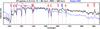 |
Fig. 1 Stack of all 277 spectra at 2 < z < 4.6 for which He II falls in the spectral region, in comparison with the composite spectrum by Shapley et al. (2003), in blue. |
2. Observations
2.1. Spectroscopy
The VVDS has exploited the high multiplex capabilities of the VIMOS instrument on the ESO-VLT (Le Fèvre et al. 2003) to collect more than 35 000 spectra of galaxies between z ~ 0 and z ~ 5 (Le Fèvre et al. 2005; Garilli et al. 2008; Le Fèvre et al., in prep.). In the VVDS-Deep 0216-04 field, more than ~10 000 spectra have been collected for galaxies with IAB ≤ 24, observed with the LR-Red grism across the wavelength range 5500 < λ < 9350 Å, with integration times of 16 000 s, over an area of 0.62 deg2. In addition, the VVDS Ultra-Deep (Le Fèvre et al., in prep.) has collected ~1000 spectra for galaxies with iAB ≤ 24.75, obtained with LR-blue and LR-red grisms, with integration times of 65 000 s for each grism, over an area of 0.16 deg2. This produces spectra with a wavelength range 3600 < λ < 9350 Å. For both the Deep and Ultra-Deep surveys, the slits have been designed to be 1′′ in width, providing a good sampling of the 1′′ typical seeing of Paranal, and between ~4′′ and ~15′′ in length, which allows for good sky determination on both sides of the main target. The resulting resolution power is R ≃ 230–250 for both the LR-blue and LR-red grisms, providing a theoretical spectral resolution of ~22 Å at 5000 Å. Using the calibration lamp emission line spectra, we measured a true resolution (FWHM) of ~22 Å, corresponding to a velocity resolution of ~1150 km s-1 at z ~ 2.5. However, as the atmospheric seeing during the observations was often better than the slit width, the galaxies in our sample never completely filled the slit: we measured on the 2D spectra the FWHM in the spatial direction for the 39 He II emitters, and we found values between 0.5′′ and 1.2′′, with a typical value of 0.8′′. These values are very similar to the FWHM of the seeing, meaning that the spectra are barely resolved in the spatial direction. Assuming that objects are circular, we can assume that their spatial extent across the slit is also 0.8′′. As a result, the effective resolution in the spectral direction can be smaller than the nominal one. We have therefore taken ~18 Å as the average spectra resolution, corresponding to ~1000 km s-1 at λ = 1640 Å at z ~ 2.5.
We deconvolved the observed line FWHM into intrinsic FWHM0 applying the simple equation 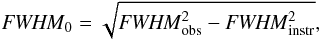 (1)where FWHMinstr is the instrumental resolution. Assuming that FWHMinstr = 1000 km s-1 (as derived from the mean spectral resolution of 18 Å reported above), an emitter with observed FWHM = 1200 km s-1 will have an intrinsic FWHM = 663 km s-1, and an emitter with observed FWHM = 2000 km s-1 will have an intrinsic FWHM = 1732 km s-1. Of course, with our assumption, the conversion is meaningless for those galaxies with observed FWHM < 1000 km s-1.
2.2. Photometry and SED fitting
The VVDS 0216-04 field benefits from extensive deep photometry. The field was first observed with the CFH12K camera in the BVRI bands (Le Fèvre et al. 2004; McCracken et al. 2003), in the U band (Radovich et al. 2004) and in the Ks band (Iovino et al. 2005). More recent and significantly deeper observations were obtained as part of the CFHT Legacy Survey in ugri and z′ (Goranova et al. 2009; Coupon et al. 2009), and as part of the WIRDS survey in J, H, and Ks bands (Bielby et al. 2012). We use the T0005 data release of the CFHTLS observations that reach 5σ point source limiting magnitudes of 26.8, 27.4, 27.1, 26.1 and 25.7 in the u∗, g′, r′, i′, and z′ bands, respectively. The WIRDS observations reach a 5σ point source limit of 24.2, 24.1, ad 24 in the J, H, and Ks bands, respctively.
Additional NIR imaging is available as a part of the Spitzer Wide-Area InfraRed Extragalactic survey (SWIRE; Lonsdale et al. 2003), providing imaging in the 3.6, 4.5, 5.8, 8.0 and 24 μm channels reaching 5σ limits of 22.8, 22.1, 20.2, 20.1 and 18.5, respectively. Moreover, Herschel data are available as a part of the Herschel Multi-tiered Extragalactic Survey (HerMES; Oliver et al. 2012): the coverage is quite shallow, giving 5σ limits of about 12 mJy in the 250, 350, and 500 μm channels.
X-ray observations of the VVDS 0216-04 field are also available as a part of the XMM Medium Deep Survey (XMDS; Chiappetti et al. 2005), reaching 3σ limits of 6 × 10-15 and 8 × 10-15 erg s-1 cm-2 in the soft and hard bands, respectively. This limit translates to about LX ~ 1044 erg s-1 cm-2 at z = 2, corresponding to a moderately powerful Seyfert.
We performed the spectral energy distribution (SED) fitting using the code ALF (Algorithm for Luminosity Function, Ilbert et al. 2005) that includes the routines of the code Le Phare1. We used the template library from Bruzual & Charlot (2003), and we also included in the fit the dust attenuation in the form defined by Calzetti et al. (2000). The SED fitting was performed on the observed u∗Bg′Vr′i′Iz′JHKs photometric broadbands. We refer the reader to Cucciati et al. (2012) for more details. Walcher et al. (2008) demonstrated that, for a sample of galaxies with spectroscopic redshift z < 1.2 drawn from the VVDS sample, the SFR inferred from a similar SED fitting procedure (though with slightly worse photometry than in this work) agrees well with the one measured via O II and/or Hα lines.
3. The He II emitters
3.1. Properties of the parent sample of star-forming galaxies at 2 < z < 4.6
In this study we concentrate on galaxies with secure redshifts (flags 2, 3, 4, 9, see Le Fèvre et al. 2005) in the range 2 < z < 4.6, for which the He II line at λrest = 1640 Å is redshifted to ~5000−9200 Å. The Ultra-Deep spectra cover this wavelength range completely, while the Deep spectra only cover this range from z = 2.3 to z = 4.6. In total, these criteria select 277 galaxies, 66 of which are from the Deep survey. The galaxies in the sample show different lines in their UV rest-frame domain, such as Lyα (1216 Å), Si II (1260 Å), O I doublet (1303 Å), C II (1334 Å), Si IV doublet (1397 Å), C IV doublet (1549 Å), Al II (1671 Å), He II (1640 Å), and C III (1909 Å). For each galaxy, the redshift was estimated by measuring the observed wavelength of the lines present in the observed spectrum. Since it has been observationally shown that Lyα is often redshifted with respect to interstellar lines (Steidel et al. 2010), Lyα was not considered a good tracer of the systemic redshift of galaxies. For each galaxy, we have at least ~3 high signal-to-noise interstellar lines to perform the redshift determination.
In Fig. 1 we report the average spectrum resulting from the stack of all the 277 galaxies at 2 < z < 4.6 for which the He II line falls in the region covered by the spectroscopy, and we compare them with the stack of about 1000 Lyman-break galaxies by Shapley et al. (2003, hereafter S03). The stack was produced running the scombine routine in IRAF, which produced a variance weighted average. The spectra normalized to the median flux density estimated between λ = 1500 Å and λ = 2000 Å. A sigma clipping algorithm (lsigma = 3, hsigma = 3) was applied during the stacking process and the spectra were combined using mean stacking.
In Table 1 we report equivalent widths and line widths (FWHM) for the most relevant absorption and emission lines of the stacked spectra. In the composite spectrum, a broad He II emission at λ = 1640 Å is evident: we measure a rest-frame equivalent width of ~1.0 Å, and FWHM ~ 1800 km s-1. The presence of the He II line in this composite implies that the He II emission is a common feature in the spectra of star forming galaxies at these redshifts. Our composite spectrum is different to the S03 composite. The main difference is the slope of the continuum: our spectrum is much redder than S03. This difference is probably due to the different selection criteria. The Lyman-break galaxy technique used in S03 tends to select bluer objects, while our flux-limited sample is unbiased with respect to the color. Moreover, the S03 composite has stronger Lyα emission, stronger P-Cygni features around N V, O I, and C IV lines, and a slightly stronger He II emission (EW0 ~ 1.5 Å).
In order to test the robustness of our stacking procedure, we experimented with other stacking parameters, varying the type of scaling used before stacking (e.g., using the mean or median, applying a moderate or strong sigma clipping, changing the region in which the continuum fluxes are evaluated, etc.). We find that the set of parameters used for our stacked spectra gives the best signal-to-noise ratio (S/N) continuum; moreover, the equivalent widths of the relevant lines are always within 20% of the values shown in Table 1.
3.2. Searching for individual galaxies with He II emission
We then visually inspected the 277 spectra to identify bona fide He II emitters responsible for the emission feature in the combined spectra. We excluded all galaxies for which the He II emission at 1640 Å falls in a spectral region dominated by bright OH airglow emission lines, which dominate the background at λ > 7500 Å, and so are not easy to subtract from the combined object+sky spectra in low-resolution spectra. We identified a preliminary list of 114 potential emitters, and we cleaned it by removing the less convincing cases (objects with lines at the location of weaker OH airglow emission, or at spectral locations with known higher background noise) which resulted in 39 bona fide He II emitters. Among these, 9 are from the DEEP survey and the remaining 30 from the Ultra-DEEP one. Three of them were identified as AGN during the redshift measurement process. In order to test the robustness of our sample and to estimate the fraction of false positive lines that could be due to a stochastic noise peak, we multiplied all of the 277 spectra by –1 and we re-checked them to look for fake He II lines. We found a list of 10 fake emitters, and after cleaning this sample as we did for the real sample, we ended up with only 2 possible emitters. This experiment shows that 5% at most of our 39 emitters could be fake detections.
For each He II emitter, we measured the equivalent width, the line flux, the line observed FWHM, and the S/N of the continuum around the He II line using the onedspec task of IRAF. We then divided the sample into four subsamples: the reliable narrow He II emitters (11 objects, with FWHMHe II < 1200 km s-1); the reliable broad He II emitters (13 objects, with FWHMHe II > 1200 km s-1); the possible He II emitters (12 objects, for which the detection is not certain, based on the line shape, position with respect to sky lines and/or the line S/N) and AGN (3 objects). We chose a discriminating observed He II FWHM of 1200 km s-1 because this corresponds to an intrinsic (deconvolved) FWHM ~ 663 km s-1, a very conservative lower limit for the line width expected in the case of W-R stars (see Sects. 4 and 4.2).
Properties of the 39 galaxies with He II in emission.
3.3. Spectro-photometric properties of the He II emitters
We report in Table 2 the photometric properties of the 39 He II emitters in the sample, together with the UV continuum slope β and width of the He II line that allowed us to classify the reliable emitters between narrow and broad. The β slopes were computed fitting a power law (Fλ ∝ λβ) to the spectra between λ = 1500 Å and λ = 2500 Å. However, for some objects (marked with an asterisk in Table 2) the continuum is barely detected and so the slope is poorly constrained. Most of the objects (27) are at 2 < z < 2.5; the highest redshift object is at redshift z ~ 4; and 4 emitters have 3.5 < z < 4.5. The He II emitters span a broad range of properties: He II is found equally in massive objects (M∗/M⊙ > 1010.5) and in less massive ones (M∗/M⊙ ~ 109), both on highly star-forming objects (SFR > 1000 M⊙ yr-1 and in normal star-forming galaxies (SFR ~ 1−10 M⊙ yr-1). The He II emitters have β slopes between –0.5 and –2.5, but we do not find any correlation between the slope and the strength of Lyα or He II lines. Moreover, we do not find any particular correlation between these properties and the width of the He II line: the only clear difference is that the narrow emitters are typically fainter (both in i′ and Ks bands) than the others. The 1 arcsec typical seeing of the CFHTLS images, corresponding to about 8 kpc at z ~ 2.5, did not allow us to perform a detailed morphological analysis; however, the 39 He II emitters have morphological properties spanning from compact to more diffuse irregular objects.
Only a few He II emitters were detected in the Spitzer-SWIRE imaging survey (ids: 910177193, 910376001, 910192939 plus the three AGN). However, these objects were detected in the first two IRAC channels only, for which we have a much deeper imaging, and not in the other two channels, which does not allow us to apply the AGN/galaxy separation based on MIR colors (Donley et al. 2012). Two objects were detected in the Herschel imaging: objects 910376001 and 20366296. The first object has a total IR luminosity LTIR = 1.8 × 10¹² L⊙. Assuming that the FIR luminosity comes only from star formation, this value corresponds to a star-formation rate of about ~300 M⊙ yr-1, not far from the estimate of ~1000 M⊙ yr-1 obtained from the SED fitting. The other object detected in SPIRE is, instead, a clear AGN, but this object was not detected in the XMM-LSS survey, implying that it is probably a star-forming object with a moderately weak AGN component. Finally, we note that none of the other He II emitters were detected in the XMM-LSS survey.
3.4. Spectral properties of the individual He II emitters
We show the spectra of the 39 He II emitters, for the four groups mentioned above, in Fig. 2 (the secure emitters with narrow He II emission), Fig. 3 (the secure emitters with broad He II emission), Fig. 4 (the three AGN) and Fig. 5 (the possible He II emitters).
For each individual spectrum we identify at least two lines, that have been used to determine the spectroscopic redshift (for about 90% of the objects we identify three or more absorption and/or emission lines). The most common feature in the spectra is the doublet Si II+C IV at 1526 Å and 1549 Å. For some of the objects coming from the Deep survey (labelled 20xxxxxxx) the Lyα region is not covered. It can be also seen that for 17 He II emitters the Lyα line is in absorption. We also remark that C IV is in absorption for all objects, except for one of the AGN; for the other two, C IV is not in the covered spectral range. However, the C IV line is often asymmetric, with the red wing sharper than the blue one, suggesting in some cases the presence of an emission component just redward of the absorption reminiscent of a P-Cygni profile.
To investigate the possible presence of these C IV P-Cygni-like profiles, we report in Figs. 6–8 the close-ups of the region around He II and C IV for the narrow, broad, and probable He II emitters, respectively. For each object, we fit a single Gaussian to the He II line, which almost always gives a good representation of the line profile except for a few broad emitters, for which the observed line is skewed towards red wavelengths. On the contrary, the absorption profile of C IV is often asymmetric, with a blue absorption wing that is much broader than the red one, and not well reproduced by a single Gaussian. To improve the quality of the fit for these cases, we have to add a second Gaussian in emission, just redward of the absorption. We then fit the C IV profile combining two Gaussians: one in absorption, centered at 1549 Å, with FWHM and flux chosen to reproduce well the blue absorption wing; and a second Gaussian in emission for which the Δ λ with respect to 1549 Å and the flux in the line are left as free parameters, while we set the FWHM of this component to the same value measured for He II (assuming that they are produced by the same region). As an output, we get the ratio between the flux of the C IV component in emission and the flux in the He II line.
From Fig. 6 it is clear that only two galaxies classified as narrow He II emitters (ids: 910265546; 910294959) need a C IV emission to improve the fit to the C IV profile. However, for object 910294959 the effect is quite marginal, with an EW of the emission component of ~0.2 Å only. In all the other cases, the C IV is either undetected (ids: 910282010; 910246547; 910191609; 910362042) or is in absorption with a symmetric profile, which does not require a second component (ids: 910167429; 910260902; 20107579; 20215115; 20198832). For the broad and probable emitters, the presence of P-Cygni-like C IV profiles is a much more frequent feature: for 11 of the 13 broad emitters a C IV emission component is needed to reproduce the C IV line profile with C IV/He II ratios going from ~0.7 to ~2 (Fig. 7). The group of probable He II emitters (Fig. 8) is a more heterogeneous population: in 7 of the 12 objects a strong C IV emission component is needed, in the remaining 5 of the 12 the C IV absorption line is quite symmetric.
From this experiment we can conclude that the narrow and broad emitters appear to have very different properties of the C IV line. While the bulk of the narrow emitters do not show any sign of P-Cygni profile, most of the broad emitters need an emission component redward of the C IV line to explain the C IV line profile.
In Fig. 9 we report the rest-frame equivalent width EW0 of the He II lines as a function of the S/N per resolution element measured in the two regions 1420–1500 Å and 1700–1800 Å. These two regions are contiguous to the He II line, and as they do not contain any spectral features, they provide a reference measurement of the continuum emission. Apart from the three AGN that have typical EW0 ~ 15–20 Å, the other He II emitters in the sample have 1 ≲ EW0 ≲ 7 Å. These values are in general agreement with the rest-frame equivalent widths of the He II line measured by Scarlata et al. (2009) for a Lyα blob at z = 2.373 (EW0(He II)~ 3.5 Å) and by Erb et al. (2010) for a low-metallicity galaxy at z ~ 2.3 EW0(He II)~ 2.7 Å. Prescott et al. (2009) found instead a nebula at z ~ 1.6 with much more powerful He II emission, with EW0(He II)~ 35 Å.
Below S/N ~ 4, the EW0 and S/N are correlated: the smaller the S/N, the higher the equivalent width. This is not surprising since objects with S/N < 4 have barely detected continua. It is also clear that narrow He II emitters have continuum S/N that is lower than that of broad emitters.
In the bottom panel of Fig. 9 we compare the continuum S/Ns of the He II emitters with the S/N of the full sample of 277 galaxies sample. Objects drawn from the UDEEP survey typically have larger S/Ns than those drawn from the DEEP survey, as expected from scaling the exposure times, with the total distribution extending from S/N = 0 (on the continuum, for emission-line only spectra) to S/N ~ 20 and peaking around S/N ~ 4. The 39 He II objects with He II emission have a S/N distribution that is similar to the distribution for the 277 parent galaxies: we found He II emission in objects with both faint and bright continua.
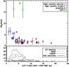 |
Fig. 9 Top panel: rest-frame equivalent width of the He II λ1640 line as a function of the average S/N per resolution element of the spectra in the two regions 1420–1500 Å and 1700–1800 Å for the 39 galaxies with detected He II in emission. The blue circles, red diamonds, black triangles, and green asterisks represent the reliable emitters with narrow He II lines, the reliable emitters with broad He II lines, the possible emitters, and the objects classified as AGN, respectively. Bottom panel: histogram of the average S/N at 1420–1500 Å and 1700–1800 Å for all 277 galaxies in the sample (long dashed line), for the DEEP and UDEEP spectra (dotted and dot-dashed, respectively), and for the 39 galaxies with He II in emission (continuous filled histogram). |
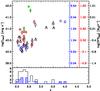 |
Fig. 10 Top panel: luminosity of the He II line as a function of the redshift for the 39 identified He II emitters in our sample. The blue circles, red diamonds, black triangles, and green stars represent the reliable emitters with narrow He II lines, the reliable emitters with broad He II lines, the possible emitters, and the objects classified as AGN, respectively. The three axes on the right represent the star-formation rates needed to produce these He II luminosities for a top-heavy IMF with Salpeter slope extending from 1 M⊙ to 500 s M⊙ with metallicities Z = 0 (black), Z = 10-7 (red), and Z = 10-5 (blue), using the conversion in Schaerer (2003) (see text). Bottom panel: redshift distribution of the 39 He II emitters (empty histogram) and of the reliable ones (filled histogram). |
In Fig. 10 we show the luminosity of the He II line as a function of the redshift for the 39 He II emitters in the sample. Two of the AGN are the most luminous objects in He II with luminosities up to 1042 erg s-1, while the other emitters have 1040 < LHe II < 1041.5 erg s-1.
In the same figure, the He II luminosities are converted to the star-formation rates needed to produce this He II emission, where it is assumed that the He II emission is due to star formation that is happening in a gas region of primeval composition. We applied three conversions calculated by Schaerer (2003): a top-heavy IMF with Salpeter slope extending from 1 M⊙ to 500 M⊙, and three metallicities Z = 0, Z = 10-7, and Z = 10-5. From these calculations we infer that, if He II originates from a region with zero metallicity, the star formation rate needed to produce the observed He II line luminosity is only 0.1−3 M⊙ yr-1. We remark also that adding just a few metals changes this estimate considerably: for Z = 10-7 and Z = 10-5 the production of He II photons is much less efficient, so we need 10 to 50 times more star formation to produce the observed He II line flux. In any case, no matter the metallicity, the SFR inferred from the He II lines under the assumption that He II is the result of star formation only are always smaller than the values measured for the individual galaxies from SED fitting (see Fig. 13).
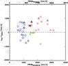 |
Fig. 11 For the 39 He II emitters, the velocity difference between the centroid of the He II line and the systemic redshift vs. the FWHM of the He II line in km s-1. The bottom axis is linear and reports the observed FWHM, while the top axis is converted in deconvoluted FWHM. The color code of the symbols is the same as in Fig. 10. |
In Fig. 11 we show the width of the He II line (FWHM, expressed in km s-1, observed and intrinsic on the bottom axis and top axis, respectively) as a function of the velocity difference between the He II line and the systemic redshift (measured from the position of the absorption lines, see Sect. 2), together with the distribution of the two quantities. The distribution of the observed FWHM extends from 600 km s-1 to 3000 km s-1, with ~10 emitters having a FWHM formally smaller than the spectral resolution of the instrument. As we explained in Sect. 2, this is not unexpected: the nominal resolution of ~1000 km s-1 has been measured on the spectra of a lamp that uniformly illuminates the 1′′ slit, while our galaxies have spatial extent of ~0.8′′ (FWHM). We conclude that galaxies with observed FWHM(He II) ≤ 1000 km s-1 are spectrally unresolved.
By our definition, the narrow and broad He II emitters have observed FWHM < 1200 and FWHM > 1200 km s-1, respectively, corresponding to intrinsic FWHM ≷ 663 km s-1. This limit has been chosen because W-R stars are always associated with strong stellar winds with speeds around or larger than 1500 km s-1; He II emitters powered by W-R stars have expected line widths around or above that limit. The possible He II emitters span a broad range of line widths, but only 3 out of 12 have FWHM > 1500 km s-1.
In Fig. 11 we also report the velocity difference Δv between the He II line and the systemic velocity, calculated measuring the position of the He II line in the rest-frame spectra. Because the systemic redshift is centered on the interstellar lines, this corresponds to the velocity difference between the He II line and those lines. We see that the reliable narrow He II emitters have ΔvHe II values spanning from –1000 to 1000 km s-1, with the distribution well centered on ΔvHe II = 0. On the other hand, reliable broad He II emitters always have ΔvHe II > 0. We ran a 2D KS test, and we found that the two distributions are different at a 90% level. This additional difference supports the hypothesis that broad and narrow He II emitters are two distinct families.
3.5. Spectral properties of stacked spectra
In order to study the average properties of broad vs. narrow vs. probable He II emitters, we produced stacked spectra for these three families of He II emitters, following the same procedure used for the composite of all the 277 He II emitters. For these composites we also experimented different stacking parameters, as previously described in Sect. 3.1, and we again find that our set of parameters gives the best and most reliable measures.
The stacked spectra are shown in Fig. 12, in comparison with stellar population models by Maraston et al. (2009) and Eldridge & Stanway (2012). We will discuss the comparison between data and models in Sect. 5. The measurements of the rest-frame equivalent width EW0 and FWHM for the relevant interstellar absorption lines are listed in Table 1.
Recently, Sommariva et al. (2012), developing a method already used by Rix et al. (2004), Halliday et al. (2008), and Quider et al. (2009), have shown that some photospheric lines in the UV rest-frame domain can be used to estimate the stellar metallicity and age. In particular, using the latest version of the Starburst99 code (Leitherer et al. 1999, 2010) they have determined the strength of five UV features (1360–1380 Å, 1415–1435 Å, 1450–1470 Å, 1496–1506 Å, and 1935–2020 Å) as a function of age and stellar metallicity. The dependence on age is very weak, with the EW of these features reaching a constant value after a few Myr only. We applied this technique to the stacks of the narrow and broad emitters, as well as to the stack of all of the 277 star forming galaxies. Some of these spectral features are very weak and noisy in our combined spectra; as a result, we obtain very different values from different lines (from 0.01 Z⊙ if the 1360–1380 Å feature is used, to 0.2 Z⊙ if 1496−1506 Å is instead used). Moreover, we do not see any difference between the values obtained for the three different stacks (broad He II emitters, narrow He II emitters, and the global sample).
The stack of the good-quality narrow He II emitters clearly shows a narrow He II emission FWHMobserved ~ 1000 km s-1 (hence unresolved at our resolution) with a rest-frame equivalent width EW ~ 4 Å comparable to those of individual spectra. The stack of the good-quality broad He II emitters also shows a broad He II line with FWHMobserved ~ 1800 km s-1 (hence 1500 km s-1 intrinsic) and EW ~ 2 Å. Interestingly, the stack of the possible He II emitters also shows a clear He II emission with EW = 3.2 Å and FWHMobserved ~ 2200 km s-1 (1960 km s-1 intrinsic).
From both a visual inspection of the composite spectra in Fig. 12 and from the analysis of the equivalent widths and line widths in Table 1 it is clear that narrow and broad He II emitters have completely different properties. The He II line width is different (FWHM ~ 1000 vs. 1600 km s-1), and the strength of the interstellar absorption lines also varies significantly between the two families. One striking difference is that the narrow He II composite spectrum has very weak low ionization interstellar lines (Si II, O I, C II, EWs ~ −1 Å) compared to the strong high ionization ones (Si IV, C IV, EWs ~ −5 Å); compared to the narrow-He II composite which shows normal low-to-high ionization ratios (similar to the ratios for the stack of all galaxies at 2 < z < 4.6). Moreover, the C IV line for the stack of the narrow emitters has a red wing absorption that is not observed in the other stacks.
4. Analysis
In the previous section we described the properties of a sample of 39 He II emitters discovered among 277 z > 2 galaxies of the VVDS Deep and Ultra-Deep surveys. In this section we analyze and discuss these properties with the aim of constraining the mechanism that produces the He II line. As discussed in the Introduction, only a few astrophysical mechanisms can power the He II nebular emission because a powerful ionizing source is needed to produce photons with energies E > 54.4 eV that can ionize He+.
4.1. AGN
The extremely blue continuum of active galactic nuclei is energetic enough to produce photons with e > 54.4 eV, thus ionizing He+ and powering the He II emission feature. Similarly to the case of W-R stars, typical spectra of AGN (both Type I and II) have other emission lines in their spectra, such as C IV and Si II, that can be used as diagnostics. Typical narrow line Type II AGN have ⟨ C IV/He II ⟩ = 1.50 (McCarthy 1993; Corbin & Boroson 1996; Humphrey et al. 2008; Matsuoka et al. 2009). Moreover, Type I AGN (those AGN in which the active nucleus is directly exposed to the observer) have line widths of 2000 km s-1 and above.
Three He II emitters in our sample have been classified as AGN. Object 910359136 has been discovered in the Ultra-Deep part of the survey, and thus is covered both with the blue and the red grism. This produces a rest-frame spectral window that covers all the spectra from Lyα to C III. The morphology of this object in the CFHTLS images is diffuse, with no point-like components, suggesting that the broad-line region is completely obscured from our line of sight. The modest line widths (FWHMobs ~ 1400 km s-1, corresponding to intrinsic FWHM0 ~ 1000 km s-1) supports this interpretation. We measure line ratios Lyα/He II = 11.5 ± 1.6, C IV/He II = 1.97 ± 0.35, and C III/C IV = 0.72 ± 0.25, that are remarkably similar to the average values for radio galaxies ⟨ Lyα/He II ⟩ = 9.8 ± 5.69 and ⟨ C IV/He II ⟩ = 1.50 ± 0.56 (McCarthy 1993; Corbin & Boroson 1996; Humphrey et al. 2008). Matsuoka et al. (2009) also found C IV/He II =  and C III/C IV =
  for narrow line regions at 2 < z < 2.5 and with 41.5 < LHe II < 42.5. We can conclude that object 910359136 is indeed a Type II AGN.
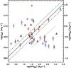 |
Fig. 13 For the 39 He II emitters, comparison between the SFR measured fitting the broad-band SED of galaxies and the luminosity of the He II line. The continuous and dashed lines show a linear best fit (with scatter) to the reliable He II emitters with broad emission (red diamonds). The dotted line is the expected correlation between these two quantities according to the cooling radiation model by Yang et al. (2006). The color code of the symbols is the same as in Fig. 10. The right axis reports the star-formation rate needed to produce this level of He II luminosity (as for Fig. 10), assuming a top-heavy IMF with Salpeter slope extending from 1 M⊙ to 500 s M⊙ and metallicity Z = 0. |
The other two objects classified as AGN (20366296 and 20273801) are instead drawn from the VVDS Deep survey, so they are only observed with the red grism, and their rest-frame spectra only cover the region between λ = 1600 Å and λ = 2600 Å, a spectral domain which covers only from He II to C III. The He II and C III lines are broad (~2000 km s-1), and the sources are point-like in the CFHTLS images; thus, it is likely that they are Type I AGN, in which the nucleus is directly exposed to the line of sight directed to the observer.
Are the remaining 36 He II emitters powered by an AGN? From a visual inspection of Figs. 6–8 it is evident that for the remaining He II emitters in our sample C IV is either undetected (910252781, 910301515, 910191609, 910362042, 20215115, 910248329, 910285698, 910246547, and 20191386) or in absorption (all the other cases). This implies C IV/He II ratios always smaller than 0.5: the ratio is an upper limit for the objects with no C IV detection and it is negative for the objects with C IV in absorption. Since in typical AGN we expect a C IV line always stronger than the He II line (McCarthy 1993; Corbin & Boroson 1996; Humphrey et al. 2008; Matsuoka et al. 2009), we can exclude the AGN as a plausible source of ionization for all 37 He II emitters. We also stress that it is very unlikely that a highly obscured AGN, like the ones discovered by Civano et al. (2011), is responsible for the He II emission in our objects. If those objects do not have in their spectra the emission lines typical of unobscured AGN because they have been absorbed by dust, there is no reason why the He II line could not have been absorbed too. Moreover, we stress that those objects for which a C IV emission component has been identified, responsible for the asymmetry of the C IV absorption profile, are unlikely to be powered by AGN: AGN in fact usually do not show P-Cygni-like line profiles in their spectra (e.g., Matsuoka et al. 2009).
Finally, it is also possible that a normal Type II AGN is buried deep inside our objects, producing at the same time the He II emission line and a C IV emission that is not visible since it would be hidden in the C IV absorption typical of the host galaxies. However, since AGN do not produce low-ionization lines such as Si II λ1527, this scenario would significantly reduce the C IV absorption while leaving Si II unchanged, ultimately altering the C IV/Si II ratio. Since we do not see objects with strange C IV/Si II ratios (i.e., objects with a stronger Si II than C IV absorption), we can exclude this possibility.
4.2. Wolf-Rayet stars
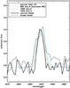 |
Fig. 14 Blow-up of the region around the He II line for the stacks of the narrow emitters (thick black line) and the broad emitters (light black line). We report the Gaussian with an observed FWHM = 1000 km s-1, the width that we measure for the He II line in the narrow stack. For comparison, we also show other Gaussians with intrinsic FWHMs of 800 km s-1 (green dashed line), 1200 km s-1 (blue dashed line) and 1500 km s-1 (cyan dashed line). These line widths, once convoluted with our 1000 km s-1 resolution, produce observed FWHM of 1250, 1500, and 1800 km s-1, respectively. |
Another possible mechanism powering He II emission is W-R stars. W-R stars are evolved and massive stars (>10 M⊙), descendents of O stars, with surface temperatures between 30 000 and 200 000 K that are losing mass very rapidly. They typically show strong and broad emission lines produced by their dense and fast stellar winds (Leitherer et al. 1995, 1996; Crowther 2007). The extremely high surface temperatures of these stars can produce the energetic photons needed to power the He II emission. The He II line width, as for the other emission lines, is expected to be broad with a FWHM on the order of few thousands of km s-1 (Schaerer 2003).
The W-R stars are commonly divided in WC, whose spectra are dominated by carbon lines, and WN stars, with spectra dominated by nitrogen lines. Both classes show strong and broad He II λ1640 emission, with typical line widths in excess of 1000 km s-1 (Crowther 2007). In WC stars the C IV λ1549/He II λ1640 ratio is always greater than one (Sander et al. 2012), while in WN stars this ratio is lower than 1, with cases with no C IV emission at all (Hamann et al. 2006). While the abundance of WC and WN stars is about the same in the Milky Way, WN are ten times more common than WC stars in low metallicity objects (Massey & Holmes 2002). In addition, Crowther & Hadfield (2006) showed that in low metallicity environments the He II flux and line width are reduced, with line FWHMs as low as 850 km s-1. Chandar et al. (2004) and Hadfield & Crowther identified the most extreme W-R galaxy in the local Universe: NGC3125 shows a strong He II line with EW ~ 7 Å and FWHM ~ 800 km s-1. The C IV emission in W-R stars often shows a P-Cygni profile, typical of the hot expanding envelope associated with this stellar phase (Crowther 2009). In Sect. 3.4 we showed that 11 out of 13 reliable broad emitters have strong indications of P-Cygni C IV line profiles (Fig. 7). This probably indicates that, for those broad emitters, the He II and C IV originate in the winds of massive W-R stars.
In Fig. 14 we show the blow-up of the region around the He II line for the narrow and broad stacks, in comparison with Gaussians with different widths, in order to evaluate the ability of our data, which have a typical velocity resolution of 1000 km s-1, of resolving the line widths for the most extreme W-R objects. We overplot a Gaussian with observed FWHM = 1000 km s-1, the width that we measure for the He II line in the stack of the narrow emitters, and that again corresponds to our spectral resolution. We also overplot a Gaussian with intrinsic FWHM = 800 km s-1 (the narrowest He II in the local Universe produced by W-R stars) that corresponds, after convolving with the instrumental resolution of 1000 km s-1, to an observed FWHM = 1250 km s-1. It is evident that this Gaussian is wider than the observed He II line, and that in principle we would be able to identify a line with such FWHM observed at our resolution. For comparison, we also report two Gaussians with observed FWHM of 1500 and 1800 km s-1, corresponding to intrinsic FWHM of 1200 and 1500 km s-1 at our resolution. The latter corresponds to the width that we measure for the He II line in the broad composite.
Including the W-R phase in stellar population synthesis models is not an easy task; the W-R phase heavily depends on the number of very massive stars (and thus on the IMF), on the atmosphere and wind models of very massive stars, and as we mentioned earlier, on the metallicity of the environment. Shapley et al. (2003), who first detected a broad He II emission in the composite of 1000 z ~ 3 galaxies, interpreted the He II line as the signature of W-R stars, but then failed to identify a stellar model that could at the same time reproduce the strength of the line and the P-Cygni C IV emission. Brinchmann et al. (2008a) combined the state-of-the-art population synthesis models with observations of local galaxies in the Sloan Digital Sky Survey, generating a model that can reproduce the observational features of the S03 composite spectrum with a half solar metallicity.
Eldridge & Stanway (2012; hereafter ES12) have recently published a grid of synthetic spectra produced using a new stellar population synthesis code that includes massive binary stars. These models naturally incorporate a W-R phase, and predict strong He II emission about 50 Myr after the burst of star formation (the age for which the number of W-R stars reaches a maximum). The strength of the He II line depends on the metallicity, and it is strongest for Z = 0.004. In the ES12 models the He II emission is broad and is always accompanied by a C IV absorption+emission P-Cygni line. Using these models and invoking a carbon reduction with respect to other metals, ES12 can reproduce quite nicely the C IV line profile and the He II emission in the S03 spectrum.
In Fig. 12 we checked whether or not we could reproduce the properties of our stacked spectra with the ES12 models. However, these models do not include interstellar absorption lines. In order to build more reasonable synthetic spectra, we decided to combine the ES12 models with the synthetic high-resolution UV spectra by Maraston et al. (2009) that conversely include interstellar lines (but no He II emission). We stress that we did not try to perform any rigorous fitting procedure, but we simply compared the predictions by a combination of these two sets of models with our composite spectra. The only restriction we imposed is that the metallicity of the components used to build our synthetic spectra is always subsolar (as it is expected to be at z ~ 2.5).
The models are superimposed to the composite spectra in Fig. 12. For the stack of the narrow He II emitters, which does not have strong low-ionization lines, we simply chose an E12 model, with a continuous star formation of 1 M⊙ yr-1 lasting 100 Myr and metallicity Z = 0.004 (but an instantaneous 10-Myr-old burst and the same metallicity produces a similar synthetic spectrum). For the broad He II emitters, we built a more complicated ad-hoc (and possibly unphysical) model: we combined a 150-Myr-old burst of star formation with metallicity Z = 0.01 from Maraston et al. (2009), with a second burst of star formation with metallicity Z = 0.004 and age = 10 Myr, from the ES12 library. Finally, for the stack of the possible emitters, we produced a similar synthetic spectrum to the one used for the broad composite, with only a slightly younger second component from the ES12 library. We stress that these are not the best possible models; rather, they are only one of the many combinations that come close to reproducing the features of our composite spectra.
Starting from the narrow composite, it is clear that the overall shape of the spectrum is reproduced well by the synthetic model. The model reproduces the absence of low-ionization lines (O I, Si II, and C II), and the strength of the Si IV absorption feature at ~1400 Å. However, the He II emission in the model is significantly broader (~2000 km s-1) than in the composite (even though the EW is similar), and the shape of the C IV line is completely different, with the model predicting a P-Cygni profile that we do not observe in the stack. We remark that other models in ES12 library are not able to reproduce the narrow He II line that we see in our composite, nor the absence of C IV P-Cygni profile. On the other hand, our ad-hoc models for the broad and possible He II emitters reproduce quite nicely the strength, shape, and width of the He II line. Moreover, the shapes of the C IV lines in the model and in the composite spectrum are qualitatively similar, and all the other absorption lines are quite well reproduced.
The outcome of this analysis is that we were unable to reproduce the properties of the narrow He II emitters with the state-of-the-art stellar population models including W-R stars. On the other hand, although more refined modeling might be required, we can reproduce the main spectral features of the broad emitters with stellar models including a specific treatment of the W-R phase.
We remark that the lack of broad He II emitters with a negative Δv between the He II line and the systemic velocity (see Fig. 11) is compatible with the W-R scenario. It is expected that if the He II emission originates in the fast winds of a W-R star, the profile of the line is the typical P-Cygni profile (Venero et al. 2002). It is also worth noting that a correlation between the star-formation rate of the galaxy and the number of W-R stars (and thus the He II luminosity) is expected for the W-R scenario, with the only caution that the W-R phase might be very short, and would not match the global star-formation rate of the galaxy. In Fig. 13 we compare the star-formation rate measured from fitting the SED of galaxies (see details in Sect. 2.2) and the luminosity of the He II line. Interestingly, we observe a correlation between the luminosity of the He II line and the star-formation rate for the galaxies in the high-quality broad emitters category (see Fig. 13), in broad agreement with predictions by models.
4.3. Gravitational cooling radiation from gas accretion
Gravitational cooling radiation from gas accreting onto dark matter haloes is another mechanism that can produce Lyα+He II emission lines, as predicted by many theoretical papers. Keres et al. (2005) showed that about half of the gas infalling onto dark matter potential is heated to temperatures T ~ 104–105 K. At these temperatures, the gas is expected to cool via line emission, in particular Lyα and He II (Yang et al. 2006). The Lyα line is in principle expected to be the strongest line, but its strength depends on the radiative transfer of Lyα photons and on the geometry and dynamics of the system; as a result, the Lyα line is easily destroyed. On the other hand, He II emission should always be observed, and its luminosity should correlate with the star-formation rate of the galaxy the gas is falling into. Intuitively, the more gas falls onto the galaxy, the higher the He II emission and thus the higher the SFR. The correlation is tighter assuming that the infalling gas is optically thin, and the predicted scatter is larger if the gas is optically thick (Yang et al. 2006).
Another prediction of this model is that the He II line is expected to have widths not larger than 300 km s-1, and the He II emission is expected to be less extended than that of the Lyα line (Yang et al. 2006; Haiman et al. 2000). However, these models assume primordial composition for the infalling gas; the presence of metals can change the cooling efficiency and thus affect the strength of the He II line.
With the spectral resolution of our observations FWHMintrinsic ~ 660 km s-1 we are only able to say that the widths of the narrow He II emitters are broadly consistent with the line width of ~300 km s-1 predicted by the models (Yang et al. 2006). Moreover, galaxies with a resolved He II line (i.e., galaxies with FWHMHe II > 1200 km s-1) are not compatible with the theoretical predictions for the cooling radiation scenario. Unfortunately, the spatial resolution of our spectra (FWHMseeing = 0.8′′ at best) does not allow us to check if the He II and Lyα emission (where present) have different spatial extents. Interestingly, we find that the C IV line profile of the narrow He II emitters in the composite spectrum shows a red absorption wing. In the context of accretion, this could be interpreted as the signature of infalling gas.
However, we saw in Fig. 13 that, for the narrow He II emitters, we do not observe any correlation between the He II luminosity and the overall star-formation rate of the galaxies, in disagreement with the predictions by Yang et al. (2006).
Another test that we can perform is to compare the number density of He II emitters above a given He II Luminosity with the predictions of the models: since the gas accretion is ubiquitous in cosmological simulations, models predict number density as high as 0.1 He II emitters per cubic Mpc at z ~ 2–3 with He II luminosity LHe II > 1040 erg/s (Yang et al. 2006). We calculated the number density of He II in our sample (excluding the broad emitters, that are probably powered by W-R stars) applying the classical V/Vmax method (Avni & Bahcall 1980), and weighting each galaxy by the photometric sampling rate (basically the ratio between the number of galaxies of a given magnitude that have been spectroscopically observed). The total volume sampled by the Ultra-Deep and Deep surveys between z = 2 and z = 3.5 is about 106.3 and 107 Mpc3, respectively. The number density that we measure for our sample is ~10-4 gal/Mpc3, thus 2–2.5 orders of magnitude smaller than the value expected by the simulations.
We conclude from this indirect argument that it seems unlikely that our 39 He II emitters are powered by cooling radiation. However, we note that to make accretion models compatible with our observations, some dramatic reduction in the cooling radiation output, by about 2 orders of magnitude, would be needed in the simulations.
4.4. PopIII star formation
Star formation in metal-free or very low metallicity regions is another mechanism that is able to produce the extremely energetic photons needed to ionize He+ and thus power the He II emission. Many authors suggested that PopIII star forming regions can be found looking for dual Lyα+He II emitters (Tumlinson et al. 2001; Schaerer 2003; Raiter et al. 2010). These models predict extremely large equivalent widths for both Lyα and He II. Schaerer (2003), for example, expects EW(Lyα) = 600–1500 Å and EW(He II)= 20–100 Å for a burst of star formation (according to the metallicity, from Z = 0 to Z = 10-5, and the IMF). However, such large EWs are sustained only for 2 Myr at the most, and the equilibrium values reached in the case of a constant star formation are much smaller: for a top-heavy IMF and extremely low metallicities (Z < 10-5), the EW for the Lyα and He II lines are ~300–400 Å and ~5–15 Å, respectively (Schaerer 2003). We remark that the equivalent width of the He II line for this model strongly depends on the metallicity, and drops to virtually zero at Z > 10-5. The typical ratio between the strength of the He II and Lyα line that the models predict also depends on the metallicity as well as the IMF: for a top-heavy IMF and zero metallicity this ratio is around He II/Lyα ~ 0.1 (Schaerer 2003; Raiter et al. 2010). Unfortunately, the Lyα is resonant, and the Lyα photons can be easily destroyed, as noted above, so the predictions for the Lyα luminosity and EW are highly uncertain.
The distribution of EW(He II) for all He II emitters in our sample (except AGN) as shown in Fig. 9 is EW ~ 1–8 Å, values that are similar to those expected for an event of continuous PopIII star formation (Schaerer 2003; Raiter et al. 2010). We showed in Fig. 10 that the SFR needed to power the He II fluxes that we observe in our galaxies are not so extreme: as long as the IMF is top-heavy (as seems reasonable for PopIII star formation) and the metallicity is close to zero we find values of 0.1–10 M⊙ yr-1.
In Fig. 13 we showed that there is no correlation between the SFR measured for the individual galaxies and the He II line luminosity. Moreover, from Fig. 13 we also showed that, assuming again that the He II emission is powered by PopIII star formation, the SFR in PopIII stars needed to generate the observed He II luminosities is always smaller (by ~2 orders of magnitude) than the SFR measured from fitting the SED. These two findings together imply that, if the nebular He II emission is really powered by PopIII star formation, it is happening in a small fraction of the volume of the galaxy containing some pristine gas and not in the galaxy as a whole. This would imply that the observed integrated spectra are a mix of two components 1) normal star-forming moderate-metallicity stellar populations comprising a majority (90%) of the SF activity; and 2) PopIII stellar populations producing the ionized He, comprising a small fraction of the global star formation. This implies that the EW of the He II line is somewhat diluted in the integrated spectrum. If the host spectrum had a continuum 100× brighter than the PopIII component at 1640 Å, the EW of the He II line in the total spectrum would be 100× smaller than the intrinsic PopIII value.
From Fig. 11 we also saw that the He II emitters in our sample show a broad range of He II line widths: 11 He II emitters have intrinsic FWHMHe II < 660 km s-1 and have velocity differences between the He II line and the system well distributed around zero. These He II emitters are not compatible with the W-R scenario in which the He II line is expected to be broadened by stellar winds, and are more compatible with the PopIII scenario. Conversely, the He II emitters with broad He II line are instead inconsistent with the PopIII scenario, which would produce narrow He II emission, and are instead more likely to be powered by W-R stars (as explained in the previous section).
Another prediction of the PopIII model that we can test is the star-formation rate density in PopIII stars at z ~ 2.5, the median redshift of our sample. Tornatore et al. (2007) predict that, although the metallicity in the center of overdensities is rapidly enriched by star formation feedback, zero metallicity regions can survive in the low-density regions around the large overdensities even down to z ~ 2. In particular, at z ~ 2.5 Tornatore et al. (2007) predict a PopIII SFRD of 3 × 10⁻⁷ M⊙ yr-1 Mpc-3. If we make the conservative assumption that only the 11 reliable He II emitters with narrow He II emission in our sample (excluding the possible He II emitters or a fraction thereof) are powered by PopIII star formation, and we use the conversion between He II Luminosity LHe II and PopIII SFR for a top-heavy IMF and zero metallicity calculated by Schaerer (2003), we get a SFRD ~ 10-6 M⊙ yr-1 Mpc-3, only a factor three above the prediction by Tornatore et al. (2007). This value is in broad agreement with the one derived by Prescott et al. (2009), who found SFRD ~ 3.3 ~ 10-7 M⊙ yr-1 Mpc-3, based on the discovery of a Lyα+He II nebula at z = 1.67. We conclude from this analysis that the SFRD derived from the observed He II assuming it is produced by PopIII stars is in broad agreement with predictions from the model of Tornatore et al. (2007), but that, if this is indeed the mechanism in place, models would need to be iterated on to match the observed SFRD.
4.5. Peculiar stellar populations
In the local Universe several HII regions showing nebular He II emission have been identified (Schaerer et al. 1999; Izotov & Thuan 1998; Guseva & Izotov 2000; Kehrig et al. 2011). For many of these regions the spectra show the features typical of W-R stars, which are thought to be the source of the strong ionizing continuum (see Sect. 4.2), but some are not clearly associated with W-R stars, nor with O-B stars (Kehrig et al. 2011).
A nebular He II component is also observed in the spectra of galaxies (de Mello et al. 1998; Izotov et al. 2006; Shirazi & Brinchmann 2012; Shapley et al. 2003; Erb et al. 2010). Once again, for many of these objects, especially at low metallicity, the nebular He II emission is not accompanied by any W-R signatures, and thus the W-R scenario can not fully explain the origin of this nebular He II emission.
The origin of the nebular He II emission in these objects is puzzling. Kudritzki (2002) showed that not only W-R, but also certain O stars are hot enough to produce nebular He II emission. Brinchmann et al. (2008a) claimed that at low metallicity the main source of nebular He II emission appears to be O stars, arguing for less dense stellar winds that can be optically thin and thus be penetrated by the ionizing photons. However, the ability of O stars to produce nebular He II emission is still debated, as some local nebulae do show narrow He II emission but no they do not seem to contain O stars neither W-R stars (Kehrig et al. 2011).
Another possibility is that at low metallicity massive stars rotate fast enough to evolve homogeneously (i.e., Meynet & Mader 2007), thus producing higher surface temperatures. However, observational evidence for this scenario has not been reported so far.
Post-AGB stars are also claimed to be able to produce nebular He II emission (Binette et al. 1994). In this scenario, these authors demonstrate that 100 million years after a strong burst of star formation, the dominating source of ionizing photons becomes post-AGB stars, and that their combined radiation field is sufficient to ionize He II. However, even assuming that our galaxies are as massive as 1011 M⊙, and that all the stellar mass has been formed during an initial burst of star formation, the He II luminosities produced by post-AGB stars would be 2–3 orders of magnitude smaller than those observed for our sample.
If the physical process responsible for nebular He II in the local universe, whatever it turns out to be, is similar to the process at work at z ~ 3, we note that there must have been a strong increase of the frequency of this phenomenon, or its timescale, as we observe more than 3% of the global galaxy population at z ~ 3 with narrow He II, while this number is much lower at z ~ 0.
4.6. Other mechanisms
Shocks by supernova driven winds have been proposed by many authors (Taniguchi & Shioya 2000; Mori et al. 2004) as the possible ionization source powering the so called Lyα blobs (Steidel et al. 2000). It is then reasonable to consider whether this mechanism can be the source of ionization producing the He II emission as well. However, fast shock models always predict C IV in emission (Dopita & Sutherland 1996; Allen et al. 2008), with C IV/He II ratios much higher than those measured for our sample (0.1 < C IV/He II < 4, depending on the shock velocity). We can therefore exclude that the bulk of our He II emitters are powered by supernova winds.
5. Discussion
In the previous sections we reviewed the mechanisms that are able to produce the very energetic photons (e > 54.4 eV) needed to ionize He+, and that can power the He II emission, and we compared what the models of these mechanisms predict with the properties of our He II emitters.
As we discussed in Sect. 4.1, apart from the three certain AGN, it is unlikely that the remaining 37 He II emitters are powered by an AGN, as C IV is always undetected or in absorption (Figs. 2, 3 and 5), while for typical narrow line regions it is expected to be in emission and always stronger than He II (McCarthy 1993; Humphrey et al. 2008). With a similar argument, we can also exclude that the source of ionizing photons are the fast winds produced by supernovae. Similar conclusions (although less robust) were drawn by Prescott et al. (2009) and Scarlata et al. (2009), who identified Lyα+He II emitters at 1.5 < z < 2.5.
Shapley et al. (2003) presented the stack of 1000 spectra of galaxies at z ~ 3, in which they detected a broad He II emission (FWHM ~ 1500 km s-1). Because of the broad He II line, and a clear signature of fast winds (i.e., the C IV P-Cygni profile in their composite), they interpreted the He II emission as evidence of a rich W-R population in their sample. More recent studies have confirmed this claim (Brinchmann et al. 2008a; Eldridge & Stanway 2012). We saw in Fig. 1 that the composite of our 277 galaxies at 2 < z < 4.6 is quite similar to the S03 composite, so we could be tempted to draw similar conclusions about the source of the He II emission.
We saw however that our He II emitters sample is quite heterogeneous, with as many objects with narrow He II emission as with broad. The two families have very different properties: the narrow He II emitters have weaker low-ionization lines (O I, C II, and Si II) than the broad ones; the narrow stack shows a red absorption wing in the C IV line that is not observed at all in the composite of the broad emitters.
From a direct comparison with modern models of stellar population synthesis that include the W-R phase (Fig. 12), we conclude that these models can reproduce, at least qualitatively, the spectral features of the composite of the broad He II emitters, mixing components of different ages and metallicities. Conversely, these models can not reproduce the main features of the narrow stack. Although with the appropriate combination of metallicity and age we can reproduce the EW of the He II line, these models always predict a broad He II line and a C IV P-Cygni line.
Another piece of information comes from the comparison of the SFR of the galaxies (measured from the SED fitting) and the He II luminosity. The broad He II emitters do show a positive correlation, as would be expected for the W-R scenario, assuming that with higher the star formation, there would be more W-R stars. No correlation at all is observed for the narrow emitters.
Putting all this evidence together, we can say that the properties of the broad He II emitters can be, at least qualitatively, explained by the W-R scenario. The narrow emitters, instead, are a different family for which the W-R scenario does not work, and thus an alternative explanation is required.
We have identified three main processes which could be the cause of the He II emission in the spectra with narrow He II emission: gravitational cooling radiation, PopIII star formation, and the presence of a peculiar stellar population. As indicated in Sect. 4.3 the He II luminosities measured from our galaxies are compatible with the ones predicted by the model by Yang et al. (2006); however, we do not see any correlation between the total SFR of the galaxies and the strength of the He II line predicted by this model. Moreover, the number density of He II emitters that we derive is at least two orders of magnitude smaller than the prediction by Yang et al. (2006). To make models compatible with our observations would therefore require either that all galaxies at these redshifts be He II emitters with EW ~ 4 A, which is excluded by our observations, or that models overpredict the number density of He II emitters by more than two orders of magnitude.
As discussed in Sect. 4.4, all observables for the narrow He II emitters are compatible with the predictions of a PopIII scenario (and this hypothesis could also be valid for some of the possible He II emitter population), if we assume that the star-formation event is happening in pockets of pristine gas that either survived at the periphery of the galaxies or has just recently accreted, hence concerning small volumes and not the full volume of the galaxies. It is quite striking that the SFRD in PopIII stars that we derive from these emitters is in broad agreement with the model by Tornatore et al. (2007) at z ~ 3, the factor of 3 difference between the two indicating that some further adjustments to the model may be necessary.
We also noted in Sect. 4.5 that various classes of objects with nebular He II emission and no W-R signatures have been identified in the local Universe. Although no convincing explanation for the origin of the He II emission has been found so far, these objects have indeed similar properties to our narrow He II emitters, and we can not exclude that they are all powered by the same mechanism. The fact that these objects are quite rare in the local Universe (Kehrig et al. 2011; Shirazi & Brinchmann 2012) and more frequent in our sample at high redshift (3–5% depending on the possible He II class, see below) may simply reflect the evolution of the star-formation rate density of the Universe (that is at its peak around the median redshift of our galaxies) and the evolution of the average metallicity of the Universe.
We were only able to compare our results with a small number of previous studies. Scarlata et al. (2009) found He II emission connected to an extended Lyα blob at z ~ 2.2. Similarly to the bulk of our emitters, they did not detect C IV nor N V in emission, as expected when the nebular emission is due to AGN activity. They concluded that the most plausible scenario for the He II emission is the cooling radiation, that can at the same time explain the width of the He II line and the lack of other emission lines. Prescott et al. (2009) also found a large Lyα+He II nebula at z ~ 1.67. However, they found a rest-frame EW for the He II line of ~35 Å, much larger than the typical values of our sample; moreover, they detect C IV in emission in their spectrum (even though weaker than He II). These two findings suggest that their object is different from the bulk of our galaxies. In the end, they can not constrain the mechanism powering the He II emission in their object. Erb et al. (2010) thoroughly analyze the UV-optical rest-frame spectrum of a galaxy at z = 2.3, in which they detect the He II line, with a rest-frame equivalent width EW0 = 2.7 Å. Thanks to their high-resolution spectroscopy (σV ~ 200 km s-1), they can study in detail the shape of the He II line, finding that 75% of the He II flux comes from a broad component (FWHM ~ 1000 km s-1) and 25% from a narrow, unresolved component. While they conclude that the broad emission probably has a stellar origin (W-R stars), the narrow emission is indicative of a hard ionizing source, possibly a very low metallicity star forming region.
To summarize, we have identified a rich population of star forming galaxies with He II emission: some show a broad He II emission, and can easily be explained by standard W-R populations; some have narrow He II emission, and they could be the high redshift counterparts of the local objects displaying nebular He II emission. Various mechanisms, more or less plausible, have been proposed to explain the He II emission in these objects (see Sect. 4.5), and in this paper we show that PopIII star formation is another mechanism that can reproduce the properties of these objects. With the current stellar population models (especially for the most massive stars and low metallicities) and with the current observations we are not able to further constrain the real mechanism.
6. Conclusions
In this paper we have reported the discovery of 39 He II λ1640 emitters, discovered in a sample of 277 VVDS galaxies with 2 < z < 4.6. Our main findings are the following:
-
1.
We showed that He II emission isa common feature in the spectra of 2 < z < 4.6 galaxies: 39/277 galaxies (14%) have He II in emission in their spectra, with EW0 = 1–7 Å. We also showed that not all of the He II emitters have Lyα in emission. On the contrary, we report for the first time the discovery of 17 He II emitters with Lyα line in absorption.
-
2.
The rest-frame EW for the He II line in our spectra is moderate; apart from three AGN, for which we find EW0 ~ 15−20, we find EW0 ~ 1–7, similar to the values expected for PopIII stars, for a continuous episode of star formation in a zero-metallicity region, assuming a top-heavy IMF, but also consistent with the EW expected for gas accretion.
-
3.
Apart from the three AGN, we never detect C IV in emission in the spectra of the He II emitters. In about 30% of the cases C IV is undetected, and in all the other cases it is in absorption. We interpret this as evidence that He II emission in most of our galaxies is not powered by AGN or supernovae winds.
-
4.
If we isolate the He II emitters with broad He II line (FWHMobs > 1200 km s-1), we do observe a correlation between the SFR of the whole galaxy (measured by fitting the UV part of the SED) and the He II line luminosity. The composite spectrum of these objects is, at least qualitatively, reproduced by stellar population synthesis models including W-R stars. We conclude that for these objects the He II emission is most likely powered by W-R stars.
-
5.
The radiation produced by gravitational cooling does not seem to play a role in producing the He II emission in our sample. For the narrow emitters, we see no correlation between the global SFR of each galaxy determined from SED fitting and the luminosity of the He II lines, as would be expected for this scenario. Moreover, we measured a number density of He II emitters with LHe II > 1040 erg s-1 of ~10-4 Mpc-3, while the predictions for the cooling radiation scenario are 2–2.5 orders of magnitude higher. This implies that either these cooling radiation simulations overestimate the number density of He II emitters, or that some mechanism somehow lowers the efficiency of the cooling radiation, which results in fainter He II fluxes.
-
6.
If we assume that the He II emission originates from a PopIII star forming region and we convert the He II luminosity into SFR using a simple recipe by Schaerer (2003), we find that a SFR of 0.1–10 M⊙ yr-1 is enough to sustain the observed He flux. The SFR derived from this PopIII hypothesis is always smaller (by 2 orders of magnitudes on average) than the global SFR measured from the SED fitting. This implies that the He II emission could originate from a relatively small volume of pristine gas which could be distributed around the galaxies, uncontaminated by metal mixing processes, and in which PopIII stars are currently forming. On the other hand, considering that PopIII star formation is powering the narrow He II emitters, as a conservative lower limit, we find a SFRD in PopIII stars of 10-6 M⊙ yr-1 Mpc-3, only 3 times higher than the value predicted at z ~ 2.5 by Tornatore et al. (2007).
-
7.
The narrow He II population has similar properties to a rare class of local objects (both individual nebulae and galaxies) which display nebular He II emission. A clear mechanism for the origin of the nebular He II line in these objects has yet to be identified, and we can not exclude that this mechanism is the low redshift tail of the PopIII star formation observed in the z ~ 3 galaxies.
Online material
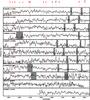 |
Fig. 2 Spectra of the reliable He II emitters with narrow He II emission (FWHM < 1000 km s-1). The grey bands show regions of the spectra that are contaminated by strong skylines or zero orders. We also report for each galaxy the id, the velocity difference between the He II and the systemic redshift, the width (FWHM) of the He II line, and the systemic redshift. |
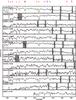 |
Fig. 3 Spectra of the reliable He II emitters with broad He II emission (FWHM > 1800 km s-1). The grey bands show regions of the spectra that are contaminated by strong skylines or zero orders. We also report for each galaxy the id, the velocity difference between the He II and the systemic redshift, the width (FWHM) of the He II line, and the systemic redshift. |
 |
Fig. 4 Spectra of the AGN with He II emission. The grey bands show regions of the spectra that are contaminated by strong skylines or zero orders. We also report for each galaxy the id, the velocity difference between the He II and the systemic redshift, the width (FWHM) of the He II line, and the systemic redshift. |
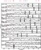 |
Fig. 5 Spectra of the possible He II emitters. The grey bands show regions of the spectra that are contaminated by strong skylines or zero orders. We also report for each galaxy the id, the velocity difference between the He II and the systemic redshift, the width (FWHM) of the He II line, and the systemic redshift. |
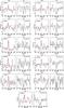 |
Fig. 6 Close-up of the region around He II (left side of each sub-figure) and around CIV (right side of each sub-figure) for each of the narrow He II emitters. In the pairs of panels, the red line shows a Gaussian fit to either He II or CIV. When a single Gaussian is not enough to reproduce the CIV absorption, we add a second Gaussian in emission (shown in blue); the resulting profile, mimicking a P-Cygni profile, is shown in green. The number in the right-side panels is the ratio between the flux of the C IV component in emission and the flux of He II. |
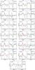 |
Fig. 7 Close-up of the region around He II (left side of each sub-figure) and around CIV (right side of each sub-figure) for each of the broad He II emitters. In the pairs of panels, the red line shows a Gaussian fit to either He II or CIV. When a single Gaussian is not enough to reproduce the CIV absorption, we add a second Gaussian in emission (shown in blue); the resulting profile, mimicking a P-Cygni profile, is shown in green. The number in the right-side panels is the ratio between the flux of the C IV component in emission and the flux of He II. |
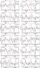 |
Fig. 8 Close-up of the region around He II (left side of each sub-figure) and around CIV (right side of each sub-figure) for each of the probable He II emitters. In the pairs of panels, the red line shows a Gaussian fit to either He II or CIV. When a single Gaussian is not enough to reproduce the CIV absorption, we add a second Gaussian in emission (shown in blue); the resulting profile, mimicking a P-Cygni profile, is shown in green. The number in the right-side panels is the ratio between the flux of the C IV component in emission and the flux of He II. |
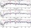 |
Fig. 12 Stack of the individual spectra for the reliable galaxies with narrow He II emission (top), the reliable galaxies with broad He II emission (middle), and the possible He II emitters (bottom). The blue lines show models obtained combining the predictions for a burst of star formation by Maraston et al. (2009) with the predictions for a Wolf-Rayet phase by Eldrige & Stanway (2012). As explained in the text, they are not an attempt of fitting the composite spectra with models, but rather are aimed at comparing some spectral features in the composite spectra with the models. |
Acknowledgments
We are very grateful to Jarle Brinchmann, Daniel Schaerer, Matthew Hayes, and Jean-Michel Deharveng for useful discussions. We also thank the anonymous referee for the constructive comments. This work is supported by funding from the ERC advanced grant ERC-2010-AdG-268107-EARLY.
References
- Allen, M. G., Groves, B. A., Dopita, M. A., et al. 2008, ApJ, 178, 20 [NASA ADS] [Google Scholar]
- Avni, Y., & Bahcall, J. N. 1980, ApJ, 235, 694 [NASA ADS] [CrossRef] [Google Scholar]
- Bielby, R., Hudelot, P., McCracken, H. J., et al. 2012, A&A, 545, A23 [NASA ADS] [CrossRef] [EDP Sciences] [Google Scholar]
- Binette, L., Magris, C. G., Stasinska, G., et al. 1994, A&A, 292, 13 [NASA ADS] [Google Scholar]
- Bouwens, R. J., Illingworth, G. D., Franx, M., & Ford, H. 2007, ApJ, 670, 928 [NASA ADS] [CrossRef] [Google Scholar]
- Bouwens, R. J., Illingworth, G. D., Franx, M., & Ford, H. 2008, ApJ, 686, 230 [NASA ADS] [CrossRef] [Google Scholar]
- Bouwens, R. J., Illingworth, G. D., Oesch, P. A., et al. 2010, ApJ, 709, 133 [Google Scholar]
- Brinchmann, J., Pettini, M., & Charlot, S. 2008a, MNRAS, 769, 782 [Google Scholar]
- Brinchmann, J., Kunth, D., & Durret, F. 2008b, A&A, 485, 657 [NASA ADS] [CrossRef] [EDP Sciences] [Google Scholar]
- Bruzual, G., & Charlot, S. 2003, MNRAS, 344, 1000 [NASA ADS] [CrossRef] [Google Scholar]
- Calzetti, D., Armus, L., Bohlin, R. C., et al. 2000, ApJ, 533, 682 [NASA ADS] [CrossRef] [Google Scholar]
- Capak, P., Mobasher, B., Scoville, N. Z., et al. 2011, ApJ, 730, 68 [NASA ADS] [CrossRef] [Google Scholar]
- Chiappetti, L., Tajer, M., Trinchieri, G., et al. 2005, A&A, 439, 413 [NASA ADS] [CrossRef] [EDP Sciences] [Google Scholar]
- Civano, F., Brusa, M., Comastri, A., et al. 2011, ApJ, 741, 91 [NASA ADS] [CrossRef] [Google Scholar]
- Corbin, M. R., & Boroson, T. A. 1996, ApJS, 107, 69 [NASA ADS] [CrossRef] [Google Scholar]
- Coupon, J., Ilbert, O., Kilbinger, M., et al. 2009, A&A, 500, 981 [NASA ADS] [CrossRef] [EDP Sciences] [Google Scholar]
- Cresci, G., Mannucci, F., Maiolino, R., et al. 2010, Nature, 467, 811 [NASA ADS] [CrossRef] [PubMed] [Google Scholar]
- Crowther, P. A. 2007, ARA&A, 45, 177 [NASA ADS] [CrossRef] [Google Scholar]
- Crowther, P. A., & Hadfield, L. J. 2006, A&A, 449, 711 [NASA ADS] [CrossRef] [EDP Sciences] [Google Scholar]
- Cucciati, O., Tresse, L., Ilbert, O., et al. 2012, A&A, 539, A31 [NASA ADS] [CrossRef] [EDP Sciences] [Google Scholar]
- Curtis-Lake, E., McLure, R. J., Pearce, H. J., et al. 2012, MNRAS, 422, 1425 [NASA ADS] [CrossRef] [EDP Sciences] [Google Scholar]
- De Mello, D. F., Schaerer, D., Heldmann, J., et al. 1998, ApJ, 507, 199 [NASA ADS] [CrossRef] [Google Scholar]
- Dekel, A., Birnboim, Y., Engel, G., et al. 2009, Nature, 457, 451 [NASA ADS] [CrossRef] [PubMed] [Google Scholar]
- Donley, J. L., Koekemoer, A. M., Brusa, M., et al. 2012, ApJ, 748, 142 [NASA ADS] [CrossRef] [Google Scholar]
- Dopita, M. A., & Sutherland, R. S. 1996, ApJS, 102, 161 [NASA ADS] [CrossRef] [Google Scholar]
- Eldridge, J. J., & Stanway, E. R. 2012, MNRAS, 419, 479 [NASA ADS] [CrossRef] [Google Scholar]
- Erb, D. K., Pettini, M., Shapley, A. E., et al. 2010, ApJ, 719, 1168 [NASA ADS] [CrossRef] [Google Scholar]
- Fardal, M. A., Katz, N., Gardner, J. P., et al. 2001, ApJ, 562, 605 [NASA ADS] [CrossRef] [Google Scholar]
- Fumagalli, M., O’Meara, J. M., & Prochaska, J. X. 2011, Science, 334, 1245 [NASA ADS] [CrossRef] [Google Scholar]
- Garilli, B., Le Fèvre, O., Guzzo, L., et al. 2008, A&A, 486, 683 [NASA ADS] [CrossRef] [EDP Sciences] [Google Scholar]
- Giavalisco, M., Vanzella, E., Salimbeni, S., et al. 2011, ApJ, 743, 95 [NASA ADS] [CrossRef] [Google Scholar]
- Goranova, Y. Hudelot, P. Magnard, F., et al. 2009, The CFHTLS T0006 Release, http://terapix.iap.fr/cplt/table_syn_T0006.html [Google Scholar]
- Guseva, N. G., Izotov, Y. I., & Thuan, T. X. 2000, ApJ, 531, 776 [NASA ADS] [CrossRef] [Google Scholar]
- Haiman, Z., Spaans, M., & Quataert, E. 2000, ApJ, 537, 5 [Google Scholar]
- Halliday, C., Daddi, E., Cimatti, A., et al. 2008, ApJ, 479, 417 [Google Scholar]
- Hamann, W.-R., Grafener, G., & Liermann, A. 2006, A&A, 457, 1015 [NASA ADS] [CrossRef] [EDP Sciences] [Google Scholar]
- Hayes, M., Schaerer, D., Ostlin, G., et al. 2011, ApJ, 730, 8 [NASA ADS] [CrossRef] [Google Scholar]
- Hibon, P., Cuby, J.-G., Willis, J., et al. 2010, A&A, 515, A97 [NASA ADS] [CrossRef] [EDP Sciences] [Google Scholar]
- Hibon, P., Kashikawa, N., Willott, C., et al. 2012, ApJ, 744, 89 [NASA ADS] [CrossRef] [Google Scholar]
- Hu, E. M., Cowie, L. L., Capak, P., et al. 2004, AJ, 127, 563 [NASA ADS] [CrossRef] [Google Scholar]
- Humphrey, P., Villar-Martin, M., Vernet, J., et al. 2008, MNRAS, 383, 11 [NASA ADS] [CrossRef] [Google Scholar]
- Ilbert, O., Tresse, L., Zucca, E., et al. 2005, A&A, 439, 863 [NASA ADS] [CrossRef] [EDP Sciences] [Google Scholar]
- Iovino, A., McCracken, H. J., Garilli, B., et al. 2005, A&A, 442, 423 [NASA ADS] [CrossRef] [EDP Sciences] [Google Scholar]
- Izotov, Y. I., & Thuan, T. X. 1998, ApJ, 500, 188 [NASA ADS] [CrossRef] [Google Scholar]
- Izotov, Y. I., Schaerer, D., Blecha, A., et al. 2006, A&A, 459, 71 [NASA ADS] [CrossRef] [EDP Sciences] [Google Scholar]
- Kehrig, C., Oey, M. S., Crowther, P. A., et al. 2011, A&A, 526, A128 [NASA ADS] [CrossRef] [EDP Sciences] [Google Scholar]
- Keres, D., Katz, N., Weinberg, D., & Davé, R. 2005, MNRAS, 363, 2 [NASA ADS] [CrossRef] [Google Scholar]
- Kudritzki, R. P. 2002, ApJ, 577, 389 [NASA ADS] [CrossRef] [Google Scholar]
- Le Fèvre, O., Saisse, M., Mancini, D., et al. 2003, SPIE, 4841, 1670 [Google Scholar]
- Le Fèvre, O., Mellier, Y., McCracken, H. J., et al. 2004, A&A, 417, 839 [NASA ADS] [CrossRef] [EDP Sciences] [Google Scholar]
- Le Fèvre, O., Vettolani, G., Garilli, B., et al. 2005, A&A, 439, 845 [NASA ADS] [CrossRef] [EDP Sciences] [Google Scholar]
- Leitherer, C., Robert, C., & Heckman, T. M. 1995, ApJS, 99, 173 [NASA ADS] [CrossRef] [Google Scholar]
- Leitherer, C., Vacca, W. D., Conti, P. S., et al. 1996, ApJ, 465, 717 [NASA ADS] [CrossRef] [Google Scholar]
- Leitherer, C., Schaerer, D., Goldader, J. D., et al. 1999, ApJ, 123, 3 [NASA ADS] [Google Scholar]
- Leitherer, C., Ortiz Otálvaro, P. A., Bresolin, F., et al. 2010, ApJS, 189, 309 [NASA ADS] [CrossRef] [Google Scholar]
- Lonsdale, C. J., Smith, H. E., Rowan-Robinson, M. P. S., et al. 1996, PASP, 115, 897 [Google Scholar]
- Malhotra, S., & Rhoads, J. E. 2002, ApJ, 565, 71 [Google Scholar]
- Maraston, C., Nieves Colmenárez, L., Bender, R., & Thomas, D. 2009, A&A, 493, 425 [NASA ADS] [CrossRef] [EDP Sciences] [Google Scholar]
- Massey, P., & Holmes, S. 2002, ApJ, 580, 35L [Google Scholar]
- Matsuoka, K., Nagao, T., Maiolino, R., et al. 2009, A&A, 503, 721 [NASA ADS] [CrossRef] [EDP Sciences] [Google Scholar]
- McCarthy, P. J. 1993, ARA&A, 31, 639 [NASA ADS] [CrossRef] [Google Scholar]
- McCracken, H. J., Radovich, M., Bertin, E., et al. 2003, A&A, 410, 17 [NASA ADS] [CrossRef] [EDP Sciences] [Google Scholar]
- McLure, R. J., Dunlop, J. S., de Ravel, L., et al. 2011, MNRAS, 418, 2074 [NASA ADS] [CrossRef] [Google Scholar]
- Meynet, G., & Maeder, A. 2007, A&A, 464, 11 [Google Scholar]
- Mori, M., Umemura, M., & Ferrara, A. 2004, ApJ, 613, 97 [Google Scholar]
- Murayama, T., Taniguchi, Y., Scoville, N. Z., et al. 2007, ApJS, 172, 523 [NASA ADS] [CrossRef] [Google Scholar]
- Nagao, T., Motohara, K., Maiolino, R., et al. 2005, ApJ, 631, 5L [Google Scholar]
- Nagao, T., Sasaki, S. S., Maiolino, R., et al. 2008, ApJ, 680, 100 [NASA ADS] [CrossRef] [Google Scholar]
- Oliver, S. J., Bock, J., Altieri, B., et al. 2012, MNRAS, 424, 1614 [NASA ADS] [CrossRef] [EDP Sciences] [Google Scholar]
- Prescott, M. K. M, Dey, A., & Jannuzi, B. T. 2009, ApJ, 702, 554 [NASA ADS] [CrossRef] [Google Scholar]
- Quider, A. M., Pettini, M., Shapley, A. E., & Steidel, C. C. 2009, ApJ, 398, 1263 [Google Scholar]
- Radovich, M., Arnaboldi, M., Ripepi, V., et al. 2004, A&A, 417, 51 [NASA ADS] [CrossRef] [EDP Sciences] [Google Scholar]
- Raiter, A., Schaerer, D., & Fosbury, R. A. E. 2010, A&A, 523, A64 [NASA ADS] [CrossRef] [EDP Sciences] [Google Scholar]
- Reuland, M., van Breugel, W., & de Vries, W. 2007, AJ, 133, 260 [Google Scholar]
- Rix, S. A., Pettini, M., Leitherer, C., et al. 2004, ApJ, 615, 98 [NASA ADS] [CrossRef] [Google Scholar]
- Sander, A., Hamann, W.-R., & Todt, H. 2012, A&A, 540, A144 [NASA ADS] [CrossRef] [EDP Sciences] [Google Scholar]
- Scarlata, C., Colbert, J., Teplitz, H. I., et al. 2009, ApJ, 706, 1241 [NASA ADS] [CrossRef] [Google Scholar]
- Schaerer, D. 2002, A&A, 382, 28 [NASA ADS] [CrossRef] [EDP Sciences] [Google Scholar]
- Schaerer, D. 2003, A&A, 397, 527 [NASA ADS] [CrossRef] [EDP Sciences] [Google Scholar]
- Schaerer, D., Contini, T., & Pindao, M. 1999, A&AS, 136, 35 [NASA ADS] [CrossRef] [EDP Sciences] [Google Scholar]
- Schenker, M. A., Stark, D. P., Ellis, R. S., et al. 2012, ApJ, 744, 179 [NASA ADS] [CrossRef] [Google Scholar]
- Shapley, A. E., Steidel, C. C., Pettini, M., et al. 2003, ApJ, 588, 65 [NASA ADS] [CrossRef] [Google Scholar]
- Shimasaku, K., Kashikawa, N., Doi, M., et al. 2006, PASJ, 58, 313 [NASA ADS] [Google Scholar]
- Shirazi, M., & Brinchmann, J. 2012, MNRAS, 421, 1043 [NASA ADS] [CrossRef] [Google Scholar]
- Sommariva, V., Mannucci, F., Cresci, G., et al. 2012, A&A, 539, A136 [NASA ADS] [CrossRef] [EDP Sciences] [Google Scholar]
- Steidel, C. C., Erb, D. K., Shapley, A. E., et al. 2010, ApJ, 717, 289 [NASA ADS] [CrossRef] [Google Scholar]
- Taniguchi, Y., & Shioya, Y. 2000, ApJ, 532, 13 [Google Scholar]
- Tapken, C., Appenzeller, I., Gabasch, A., et al. 2006, A&A, 455, 145 [NASA ADS] [CrossRef] [EDP Sciences] [Google Scholar]
- Tornatore, L., Ferrara, A., & Schneider, R. 2007, MNRAS, 382, 945 [NASA ADS] [CrossRef] [Google Scholar]
- Tumlinson, J., & Shull, J. M. 2000, ApJ, 528, 65L [Google Scholar]
- Tumlinson, J., Giroux, M. L., & Shull, J. M. 2001, ApJ, 550, 1L [Google Scholar]
- Vanzella, E., Giavalisco, M., Dickinson, M., et al. 2009, ApJ, 695, 1163 [NASA ADS] [CrossRef] [Google Scholar]
- Venero, R. O. J., Cidale, L. S., & Ringuelet, A. E. 2002, ApJ, 578, 450 [Google Scholar]
- Walcher, C. J., Lamareille, F., Vergani, D., et al. 2008, A&A, 491, 713 [NASA ADS] [CrossRef] [EDP Sciences] [Google Scholar]
- Yang, Y., Zabludoff, A. I., Davé, R., et al. 2006, ApJ, 640, 539 [NASA ADS] [CrossRef] [Google Scholar]
All Tables
All Figures
|
Fig. 1 Stack of all 277 spectra at 2 < z < 4.6 for which He II falls in the spectral region, in comparison with the composite spectrum by Shapley et al. (2003), in blue. |
| In the text | |
|
Fig. 9 Top panel: rest-frame equivalent width of the He II λ1640 line as a function of the average S/N per resolution element of the spectra in the two regions 1420–1500 Å and 1700–1800 Å for the 39 galaxies with detected He II in emission. The blue circles, red diamonds, black triangles, and green asterisks represent the reliable emitters with narrow He II lines, the reliable emitters with broad He II lines, the possible emitters, and the objects classified as AGN, respectively. Bottom panel: histogram of the average S/N at 1420–1500 Å and 1700–1800 Å for all 277 galaxies in the sample (long dashed line), for the DEEP and UDEEP spectra (dotted and dot-dashed, respectively), and for the 39 galaxies with He II in emission (continuous filled histogram). |
| In the text | |
|
Fig. 10 Top panel: luminosity of the He II line as a function of the redshift for the 39 identified He II emitters in our sample. The blue circles, red diamonds, black triangles, and green stars represent the reliable emitters with narrow He II lines, the reliable emitters with broad He II lines, the possible emitters, and the objects classified as AGN, respectively. The three axes on the right represent the star-formation rates needed to produce these He II luminosities for a top-heavy IMF with Salpeter slope extending from 1 M⊙ to 500 s M⊙ with metallicities Z = 0 (black), Z = 10-7 (red), and Z = 10-5 (blue), using the conversion in Schaerer (2003) (see text). Bottom panel: redshift distribution of the 39 He II emitters (empty histogram) and of the reliable ones (filled histogram). |
| In the text | |
|
Fig. 11 For the 39 He II emitters, the velocity difference between the centroid of the He II line and the systemic redshift vs. the FWHM of the He II line in km s-1. The bottom axis is linear and reports the observed FWHM, while the top axis is converted in deconvoluted FWHM. The color code of the symbols is the same as in Fig. 10. |
| In the text | |
|
Fig. 13 For the 39 He II emitters, comparison between the SFR measured fitting the broad-band SED of galaxies and the luminosity of the He II line. The continuous and dashed lines show a linear best fit (with scatter) to the reliable He II emitters with broad emission (red diamonds). The dotted line is the expected correlation between these two quantities according to the cooling radiation model by Yang et al. (2006). The color code of the symbols is the same as in Fig. 10. The right axis reports the star-formation rate needed to produce this level of He II luminosity (as for Fig. 10), assuming a top-heavy IMF with Salpeter slope extending from 1 M⊙ to 500 s M⊙ and metallicity Z = 0. |
| In the text | |
|
Fig. 14 Blow-up of the region around the He II line for the stacks of the narrow emitters (thick black line) and the broad emitters (light black line). We report the Gaussian with an observed FWHM = 1000 km s-1, the width that we measure for the He II line in the narrow stack. For comparison, we also show other Gaussians with intrinsic FWHMs of 800 km s-1 (green dashed line), 1200 km s-1 (blue dashed line) and 1500 km s-1 (cyan dashed line). These line widths, once convoluted with our 1000 km s-1 resolution, produce observed FWHM of 1250, 1500, and 1800 km s-1, respectively. |
| In the text | |
|
Fig. 2 Spectra of the reliable He II emitters with narrow He II emission (FWHM < 1000 km s-1). The grey bands show regions of the spectra that are contaminated by strong skylines or zero orders. We also report for each galaxy the id, the velocity difference between the He II and the systemic redshift, the width (FWHM) of the He II line, and the systemic redshift. |
| In the text | |
|
Fig. 3 Spectra of the reliable He II emitters with broad He II emission (FWHM > 1800 km s-1). The grey bands show regions of the spectra that are contaminated by strong skylines or zero orders. We also report for each galaxy the id, the velocity difference between the He II and the systemic redshift, the width (FWHM) of the He II line, and the systemic redshift. |
| In the text | |
|
Fig. 4 Spectra of the AGN with He II emission. The grey bands show regions of the spectra that are contaminated by strong skylines or zero orders. We also report for each galaxy the id, the velocity difference between the He II and the systemic redshift, the width (FWHM) of the He II line, and the systemic redshift. |
| In the text | |
|
Fig. 5 Spectra of the possible He II emitters. The grey bands show regions of the spectra that are contaminated by strong skylines or zero orders. We also report for each galaxy the id, the velocity difference between the He II and the systemic redshift, the width (FWHM) of the He II line, and the systemic redshift. |
| In the text | |
|
Fig. 6 Close-up of the region around He II (left side of each sub-figure) and around CIV (right side of each sub-figure) for each of the narrow He II emitters. In the pairs of panels, the red line shows a Gaussian fit to either He II or CIV. When a single Gaussian is not enough to reproduce the CIV absorption, we add a second Gaussian in emission (shown in blue); the resulting profile, mimicking a P-Cygni profile, is shown in green. The number in the right-side panels is the ratio between the flux of the C IV component in emission and the flux of He II. |
| In the text | |
|
Fig. 7 Close-up of the region around He II (left side of each sub-figure) and around CIV (right side of each sub-figure) for each of the broad He II emitters. In the pairs of panels, the red line shows a Gaussian fit to either He II or CIV. When a single Gaussian is not enough to reproduce the CIV absorption, we add a second Gaussian in emission (shown in blue); the resulting profile, mimicking a P-Cygni profile, is shown in green. The number in the right-side panels is the ratio between the flux of the C IV component in emission and the flux of He II. |
| In the text | |
|
Fig. 8 Close-up of the region around He II (left side of each sub-figure) and around CIV (right side of each sub-figure) for each of the probable He II emitters. In the pairs of panels, the red line shows a Gaussian fit to either He II or CIV. When a single Gaussian is not enough to reproduce the CIV absorption, we add a second Gaussian in emission (shown in blue); the resulting profile, mimicking a P-Cygni profile, is shown in green. The number in the right-side panels is the ratio between the flux of the C IV component in emission and the flux of He II. |
| In the text | |
|
Fig. 12 Stack of the individual spectra for the reliable galaxies with narrow He II emission (top), the reliable galaxies with broad He II emission (middle), and the possible He II emitters (bottom). The blue lines show models obtained combining the predictions for a burst of star formation by Maraston et al. (2009) with the predictions for a Wolf-Rayet phase by Eldrige & Stanway (2012). As explained in the text, they are not an attempt of fitting the composite spectra with models, but rather are aimed at comparing some spectral features in the composite spectra with the models. |
| In the text | |
Current usage metrics show cumulative count of Article Views (full-text article views including HTML views, PDF and ePub downloads, according to the available data) and Abstracts Views on Vision4Press platform.
Data correspond to usage on the plateform after 2015. The current usage metrics is available 48-96 hours after online publication and is updated daily on week days.
Initial download of the metrics may take a while.