| Issue |
A&A
Volume 556, August 2013
|
|
|---|---|---|
| Article Number | A62 | |
| Number of page(s) | 13 | |
| Section | Interstellar and circumstellar matter | |
| DOI | https://doi.org/10.1051/0004-6361/201220905 | |
| Published online | 29 July 2013 | |
High-angular resolution observations towards OMC-2 FIR 4: Dissecting an intermediate-mass protocluster⋆
1
UJF – Grenoble 1/CNRS–INSU, Institut de Planétologie et d’Astrophysique de
Grenoble (IPAG) UMR 5274, 38041
Grenoble, France
e-mail:
This email address is being protected from spambots. You need JavaScript enabled to view it.
2
Osservatorio Astrofisico di Arcetri, Largo E. Fermi 5, 50124
Firenze,
Italy
3
Astronomical Institute Anton Pannekoek, University of
Amsterdam, PO BOX
94249
1090 GE
Amsterdam, The
Netherlands
4
Department of Astrophysics/IMAPP, Radboud University
Nijmegen, 6525 AJ
Nijmegen, The
Netherlands
5
Université de Toulouse, UPS–OMP, IRAP,
31028
Toulouse Cedex 4,
France
6
CNRS, IRAP, 9
Av. Colonel Roche, BP
44346, 31028
Toulouse Cedex 4,
France
7
Observatorio Astronómico Nacional, PO Box 112, 28803
Alcalá de Henares, Madrid, Spain
8
Institute of Astronomy and Astrophysics, Academia
Sinica, PO Box
23-141, 106
Taipei,
Taiwan
9
Harvard–Smithsonian Center for Astrophysics,
60 Garden Street, Cambridge, MA
02138,
USA
10
IRAM, 300 rue
de la piscine, 38406 Saint-Martin d’Hères, France
11
Nobeyama Radio Observatory, 462-2 Nobeyama, Minamimaki, Minamisaku, 384-1305
Nagano,
Japan
Received:
13
December
2012
Accepted:
16
April
2013
Abstract
Context. Intermediate-mass stars are an important ingredient of our Galaxy and a key to understanding how high- and low-mass stars form in clusters. One of the closest known young intermediate-mass protoclusters is OMC-2 FIR 4, which is located at a distance of 420 pc in Orion. This region is one of the few where the complete 500–2000 GHz spectrum has been observed with the heterodyne spectrometer HIFI on board the Herschel satellite, and unbiased spectral surveys at 0.8, 1, 2, and 3 mm have been obtained with the JCMT and IRAM 30-m telescopes.
Aims. We aim to disentangle the core multiplicity, to investigate the morphology of this region in order to study the formation of a low- and intermediate-mass protostar cluster, and to aid in interpretation of the single-dish line profiles already in our hands.
Methods. We used the IRAM Plateau de Bure Interferometer to image OMC-2 FIR 4 in the 2-mm continuum emission, as well as in DCO+(2–1), DCN(2–1), C34S(3–2), and several CH3OH lines. In addition, we analysed observations of the NH3(1, 1) and (2, 2) inversion transitions that used the Very Large Array of the NRAO. The resulting maps have an angular resolution that allows us to resolve structures of 5″, which is equivalent to ~2000 AU.
Results. Our observations reveal three spatially resolved sources within OMC-2 FIR 4, of one or several solar masses each, with hints of further unresolved substructure within them. Two of these sources have elongated shapes and are associated with dust continuum emission peaks, thus likely containing at least one molecular core each. One of them also displays radio continuum emission, which may be attributed to a young B3–B4 star that dominates the overall luminosity output of the region. The third identified source displays a DCO+(2–1) emission peak and weak dust continuum emission. Its higher abundance of DCO+ relative to the other two regions suggests a lower temperature, hence its possible association with either a younger low-mass protostar or a starless core. It may alternatively be part of the colder envelope of OMC-2 FIR 4.
Conclusions. Our interferometric observations show the complexity of the intermediate-mass protocluster OMC-2 FIR 4, where multiple cores, chemical differentiation, and an ionised region all coexist within an area of only 10 000 AU.
Key words: ISM: individual objects: OMC-2 FIR 4 / ISM: molecules
Based on observations carried out with the IRAM Plateau de Bure Interferometer. IRAM is supported by the INSU/CNRS (France), MPG (Germany), and IGN (Spain).
© ESO, 2013
1. Introduction
Star formation starts in dense fragments within clouds of molecular gas and dust and ends when nuclear hydrogen burning begins at the centre of a newly formed star. During this evolution, the physical processes and different phases involved are not necessarily the same for stars of all masses. Indeed, in the field of star formation, there has traditionally been a division between low-mass stars (M ≲ 2 M⊙), intermediate-mass (IM) stars (2 M⊙ < M ≲ 8 M⊙), and high-mass stars (M > 8 M⊙).
In the past decades, most of the attention has been devoted to the study of low-mass and high-mass star formation, revealing differences between the two that are not only dynamical (Beuther et al. 2007; Zinnecker & Yorke 2007), but also chemical in nature (Bottinelli 2006; Ceccarelli et al. 2007). The formation of IM stars represents the bridge between low-mass and high-mass star formation and can bring important pieces of information to understanding how differently the process of star formation works in the two mass extremes. As their high-mass counterparts, IM stars emit a non-negligible amount of radiation in the far ultraviolet (FUV), and are thus able to photodissociate and ionise their surroundings. Therefore, the study of IM star formation can aid the current debate on the formation mechanism of high-mass stars (see Zinnecker & Yorke 2007, for a review).
While low-mass stars may form in isolation or in loose stellar aggregates, high-mass stars are always seen to be formed in densely clustered environments. IM star formation also occurs in clustered mode (e.g. Fuente et al. 2007) and has been found to be the transition between loose low-mass aggregations and tight high-mass clusters (Testi et al. 1999). IM protoclusters represent excellent laboratories for studying clustered star formation at almost the full range of stellar masses. Observationally, they can typically be found closer (d ≲ 1 kpc) than high-mass protoclusters, and they are also less complex.
Despite all this, relatively little work has focussed on the early stages of IM star formation. Only a few individual sources have been studied in detail (e.g. Fuente et al. 2009; Crimier et al. 2009, 2010; Sánchez-Monge et al. 2010; Palau et al. 2011; van Kempen et al. 2012), and therefore much remains unknown about the formation and first evolutionary stages of these objects.
The present work focusses on the IM protocluster OMC-2 FIR 4, which has a luminosity that has been reported to be between 50 L⊙ (Adams et al. 2012) and 1000 L⊙ (Crimier et al. 2009). It is located in the Orion A complex, 2 pc north of the famous Orion Nebula (M42) and the Trapezium OB association, and lies ~420 pc away from the Sun (Menten et al. 2007; Kim et al. 2008).
Thanks to its relative proximity, multiple studies have been carried out towards this region and the OMC-2/3 filament where it is located. These include continuum observations at several wavelengths (e.g. Chini et al. 1997; Johnstone & Bally 1999; Nielbock et al. 2003) and various molecular line studies (e.g. Tatematsu 1993; Cesaroni & Wilson 1994; Takahashi et al. 2008; Tatematsu et al. 2008; Liu et al. 2011; Li et al. 2012). Most of them, however, are coarse angular-resolution observations, which are very useful for investigating the overall structure of the whole filament, but not sufficient to resolve the substructure within the OMC-2 FIR 4 region. The only dedicated interferometric observations towards this source are Very Large Array (VLA) maps carried out at 3.6 cm by Reipurth et al. (1999) and a recent study conducted with the Nobeyama Millimeter Array (NMA) at 3 mm by Shimajiri et al. (2008; hereafter S08). The latter reveal several cores and the authors speculate that an external outflow driven by the nearby FIR 3 is responsible for triggering fragmentation in FIR 4, highlighting the complexity of this region.
OMC-2 FIR 4 is also one of the targets of the Herschel1 guaranteed time key programme Chemical HErschel Surveys of Star forming regions (CHESS2; Ceccarelli et al. 2010; Kama et al. 2012), which has conducted unbiased spectral surveys with the HIFI spectrometer (de Graauw et al. 2010) of eight star-forming regions, each representative of a particular aspect of the star formation process: evolutionary stage, mass of the forming star, or interaction with the surroundings. The HIFI half-power beam width ranges between 11″ at 1900 GHz and 41″ at 500 GHz, thus covering most, if not all, the area of OMC-2 FIR 4. High-angular resolution observations are therefore a crucial tool for disentangling the information hidden in the HIFI line profiles.
With this in mind, we report 2-mm continuum and line observations performed with the IRAM Plateau de Bure Interferometer (PdBI) and ammonia maps obtained with the VLA towards OMC-2 FIR 4. We describe these observations in Sect. 2; in Sect. 3 we present the maps and spectra obtained, which we discuss and interpret in Sect. 4. Finally, Sect. 5 summarises the main conclusions of this work.
2. Observations
2.1. Plateau de Bure observations
We observed OMC-2 FIR 4 with the IRAM Plateau de Bure Interferometer (PdBI) in two tracks on 15 October 2010 and 15 April 2011, using the most compact D and C configurations of the array. The data presented in this paper cover a spectral window of 1.8 GHz obtained with the WIDEX correlator, whose channel spacing is 1.95 MHz (~4 km s-1), centred on a frequency of 143.4 GHz. The phase centre of the observations is α(J2000) = 05h35m26.971s, δ(J2000) = –05°09′56.77′′. The systemic velocity of OMC-2 FIR 4 is VLSR = 11.4 km s-1.
The bandpass of the receivers was calibrated by observing 0923+392 in Oct. 2010 and NRAO150 in Apr. 2011 with flux densities of 3.55 Jy and 2.53 Jy, respectively. Amplitude and phase calibrations were achieved by monitoring 0430+052 and 0528+134, whose flux densities were determined to be 1.32 and 1.67 Jy, respectively, at 143.4 GHz. The uncertainty in the amplitude calibration is estimated to be 30%.
The data were calibrated and analysed with the GILDAS3 software package developed at IRAM and the Observatoire de Grenoble. We
obtained continuum maps from the line-free channels and subtracted the continuum from the
line emission directly in the (u, v)-domain. The
resulting 1σ rms and beam size for the naturally weighted continuum map
are 4.9 mJy beam-1 and  , respectively (see Table 1). The maps presented in this paper are not corrected
for the primary beam, but we did apply the correction to measure the reported fluxes.
, respectively (see Table 1). The maps presented in this paper are not corrected
for the primary beam, but we did apply the correction to measure the reported fluxes.
2.2. Very Large Array ammonia observations
The Very Large Array (VLA4) was used to observe the ammonia (J, K) = (1, 1) and (2, 2) inversion transitions simultaneously (project AC556). Twenty adjacent pointing centres, covering OMC-2 and OMC-3 regions, were carried out on 29 July 2000 and 24 September 2000, with the array in the D (compact) configuration. The FWHM of the primary beam at the frequency of the observations is approximately 2′, and the field centres were separated by 1′ to ensure full sampling. Each field was observed for a total on-source integration time of approximately 30 min. The absolute flux scale was set by observing the quasar 1328+307 (3C 286), for which we adopted a flux of 2.5 Jy. The quasars 0605−085 and 0539−057 with bootstrapped fluxes of 2.4 Jy and 1.0 Jy, respectively, were observed regularly to calibrate the gains and phases. Bandpass calibration was performed by observing the bright quasar 0316+413 (3C84) with a flux density of 14.2 Jy (for July) and 17.5 Jy (for September).
The data reduction followed the VLA standard guidelines for calibration of high-frequency data, using the NRAO package AIPS. The NH3 (1, 1) and NH3 (2, 2) lines were observed simultaneously in the four IF correlator modes of the VLA (with two polarisations for each line), providing 63 channels with a spacing of 0.62 km s-1 across a bandwidth of 3.125 MHz, plus an additional continuum channel containing the central 75 per cent of the total bandwidth. The bandwidth was centred at the systemic velocity VLSR = 11.4 km s-1.
Calibrated uv-data were loaded in the software MIRIAD (Sault et al. 1995) to perform the
imaging. While the continuum emission was found to be negligible (we measured an upper
limit of about 2 mJy at the frequency of the observations), we subtracted any possible
related contribution from line-free channels using the task UVLIN.
We combined and imaged the data from the central part of the mosaic, covering the OMC-2
region, with the task MOSSDI. The rms noise in the naturally
weighted maps is 5 mJy beam-1 per 0.62 km s-1 channel. We applied a
uv-taper function of 60 kλ (3″ in the image plane) to
improve the signal-to-noise ratio (S/N). The resulting synthesised beam is
 , with PA = −5°.
3. Results
3.1. Millimetre continuum emission
Figure 1 shows our PdBI naturally and uniformly weighted 2-mm continuum maps. For comparison, these are overlaid on the 3-mm continuum images obtained by S08 with the Nobeyama Millimeter Array (NMA). From their uniformly weighted image, S08 identify 11 cores at 3 mm within OMC-2 FIR 4, whose positions according to their Table 4 are marked in the figure. The parameters of our continuum observations and those of S08 are listed in Table 1.
The PdBI images allow us to resolve two elongated structures in OMC-2 FIR 4, separated by ~5″, surrounded by more extended emission that covers a total size of about 15″. The uniform map suggests the presence of additional fragmentation that cannot be completely resolved at the angular resolution of the observations. On the other hand, the NMA images display fainter, more complex, and more extended emission, which is largely below the 3σ level (first contour) in the case of the uniform map.
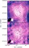 |
Fig. 1 Interferometric continuum maps of OMC-2 FIR 4 with natural (top) and uniform weighting (bottom). White contours represent the 2-mm continuum emission obtained with the PdBI, while black contours, as well as the background colour scale, correspond to the 3-mm continuum emission seen with the NMA (S08). Contours for both the PdBI and NMA maps start at 3σ and increase by steps of 3σ. The bottom-left ellipses represent the respective beam sizes. The white open circles mark the primary beam FWHM for the PdBI observations. The black crosses mark the NMA 3-mm cores as reported in Table 4 of S08. |
Lines observed with the PdBI and VLA interferometers.
It is worth mentioning that the primary beam size of our PdBI observations is 35″, so considerably smaller than that of the NMA maps, which is 82″. Similarly, the shortest baseline attained with the NMA is 2.9 kλ while that of the PdBI is 10 kλ. This results in a higher sensitivity of the NMA to extended structures. More specifically, our shortest baseline implies that our observations are sensitive to structures smaller than 17″ down to a level of 10% (see Eq. (A.8) in Wilner & Welch 1994; or Eq. (A.6) in Palau et al. 2010), while for the NMA images, this number is as high as 56″. Thus, we are not sensitive to the cores identified by S08 that fall outside the outermost PdBI contour. In spite of this, we still have several concerns regarding the core identification made by S08. First, it was based on the uniform map, which has a low S/N; second, the coordinates given for some of the cores do not coincide with the corresponding emission peak positions in the image; and third, two pairs of cores lie within a beam size of each other. We believe the NMA natural map is more reliable than the uniform one given its higher sensitivity. This already shows a number of clearly separated cores, some of which appear to be followed also by the PdBI contours. In conclusion, even though we prefer to be cautious about the reality of the 11 cores reported in S08, we are convinced that OMC-2 FIR 4 is composed of several cores. Based on our PdBI maps, we hereafter refer to the dominant eastern region as the main source, and to the western one as west source.
The continuum fluxes, which are measured inside the 5σ contour of the
corresponding maps, are 1.06 ± 0.32 Jy and 1.10 ± 0.33 Jy for the natural and uniform
maps, respectively. We can estimate the mass of the emitting clump by considering that all
the flux is emitted by dust. This is a reasonable assumption, since Reipurth et al. (1999) reported a 3.6-cm flux of 0.64 mJy for OMC-2 FIR
4 (see Sect. 4.3), and therefore the contribution of
free-free emission at 2 mm is negligible, i.e. about three orders of magnitude below the
total flux we measure. Assuming that the dust emission is optically thin, the mass,
Mdust is given by 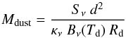 (1)where
Sν is the flux we meaure inside the
5σ contour at 2 mm, d the distance to OMC-2 FIR 4,
Td the dust temperature (adopted to be 50 K from S08),
Bν(Td) the
Planck black body function for a temperature Td, and
Rd the dust-to-gas ratio, assumed equal to 0.01. The
equation
(1)where
Sν is the flux we meaure inside the
5σ contour at 2 mm, d the distance to OMC-2 FIR 4,
Td the dust temperature (adopted to be 50 K from S08),
Bν(Td) the
Planck black body function for a temperature Td, and
Rd the dust-to-gas ratio, assumed equal to 0.01. The
equation  is the
frequency-dependent dust mass opacity coefficient. Chini et al. (1997) derived β = 2 from the spectral energy
distribution (SED) fit towards OMC-2 FIR 1 and FIR 2. Since FIR 4 is in the same molecular
filament as FIR 1 and FIR 2, we have adopted β = 2, and
κ0 = 1 cm2 g-1 at
ν0 = 250 GHz (Ossenkopf & Henning 1994).
is the
frequency-dependent dust mass opacity coefficient. Chini et al. (1997) derived β = 2 from the spectral energy
distribution (SED) fit towards OMC-2 FIR 1 and FIR 2. Since FIR 4 is in the same molecular
filament as FIR 1 and FIR 2, we have adopted β = 2, and
κ0 = 1 cm2 g-1 at
ν0 = 250 GHz (Ossenkopf & Henning 1994).
The resulting mass, from the naturally-weighted 2-mm continuum map, is 9 ± 3 M⊙. This should be considered as a lower limit to the total mass of OMC-2 FIR 4 (dense cores plus envelope), since a percentage of the total flux is expected to be filtered out by the interferometer. We can estimate the fraction of flux lost with the aid of the work published by Crimier et al. (2009), who modelled the SED function observed towards OMC-2 FIR 4 at infrared and sub-millimetre wavelengths. The flux they predict at 2 mm is 2 Jy, implying a flux loss of 45% in our PdBI continuum observations.
Crimier et al. (2009) have derived a mass of 30 M⊙ for the envelope of OMC-2 FIR 4, i.e. higher than our estimate by a factor 3. While this difference may be partly due to the loss of flux in our interferometric maps, we note that a different choice of dust temperature in Eq. (1) can significantly change the obtained mass. For example, adopting Td = 20 K, which is a reasonable dust temperature for the source outer envelope (Lis et al. 1998; Jørgensen et al. 2006; Crimier et al. 2009), yields a mass of 26 M⊙.
3.2. Line emission
The list of detected transitions are presented in Table 2, together with the 1σ rms values of the corresponding velocity channel maps (see Sects. 3.2.1 and 3.2.2). Out of the nine methanol lines detected, eight are blended due to the poor spectral resolution of the observations. Therefore, the methanol maps shown in this paper correspond to the only isolated transition we observe, i.e. CH3OH(3, 1, +0 – 2, 1, +0) at 143.87 GHz, whose upper level energy is 28 K and which is hereafter referred to as CH3OH for simplicity.
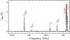 |
Fig. 2 PdBI spectrum obtained towards the phase centre of OMC-2 FIR 4 with the WIDEX correlator. The species of the detected lines are labelled. |
3.2.1. PdBI molecular line spectra and maps
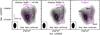 |
Fig. 3 Velocity-integrated PdBI contour maps obtained towards OMC-2 FIR 4, overlaid on the naturally weighted continuum map (grey scale). The bottom-left ellipse in each panel represents the beam size. Left: CH3OH(3, 1, +0 – 2, 1, +0) (black) and C34S(3–2) (magenta). Centre: DCN(2–1) (black) and DCO+(2–1) (magenta). All the contours start at 3σ and increase by steps of 3σ. The 1σ rms values are 0.16, 0.14, 0.17, and 0.08 Jy beam-1 km s-1, respectively for the CH3OH, C34S(3–2), DCN(2–1), and DCO+(2–1) integrated maps. Right: Polygons representing the three differentiated components, main, west, and south (see text), used to extract average spectra. The white crosses mark the positions of the three sources identified in this work (see Table 4). |
The 1.8-GHz wide spectrum obtained at the peak coordinates of OMC-2 FIR 4 with the WIDEX correlator at PdBI is presented in Fig. 2, where the detected species are labelled. Since we are also in possession of IRAM 30-m single-pointing data towards the same source (López-Sepulcre et al., in prep.), we provide in Table 3 an estimate of the velocity-integrated flux loss for each PdBI line. This ranges from 13% for CH3OH to 73% for DCO+(2–1), and indicates the presence of an important contribution from extended emission in these tracers that is filtered out by the interferometer.
Flux loss for the PdBI molecular lines.
Given the low spectral resolution of the WIDEX spectrum (1.95 MHz, i.e. 4 km
s-1), it is not possible to analyse the shape of the line profiles.
However, this is beyond the scope of the present work, which primarily aims at
investigating the spatial distribution of the emission in the different tracers. To this
end we provide, for each millimetre molecular tracer, velocity-integrated maps in Fig.
3, and velocity channel maps in Fig. 4. The synthesised beam size of these images is
4 8 × 27, and is depicted
on the bottom left-hand corner of each panel in the figures.
8 × 27, and is depicted
on the bottom left-hand corner of each panel in the figures.
OMC-2 FIR 4 sources: coordinates and fractional fluxes for each tracer.
If we focus first on the integrated maps (Fig. 3), the morphological complexity of the source becomes evident from a comparison of the emission distribution in the different tracers:
-
The CH3OH emission is dominated by the main source (see Sect. 3.1 above), which displays an elongated shape, and shows hints of a secondary component towards the west (the above mentioned west source), mimicking the spatial distribution of the 2-mm continuum emission. This morphology does not change when seen in the blended CH3OH lines around 145 GHz.
-
C34S(3–2) displays a more compact emission that traces both the main and west sources.
-
The DCN(2–1) emission peaks at the main source, but it expands towards the west and the north, following the elongated morphology of the west source as seen in the continuum images.
-
DCO+(2–1) peaks to the south of the main and west sources, a different region that we name south source, which is not traced well by any other line.
In summary, from the integrated maps we conclude that each molecular line traces the region differently. We differentiate three spatially separated emission components, which we have named main, west, and south sources, lying ~0.01 pc (i.e. 2000 AU) apart from each other. These regions are schematically depicted in the right-hand panel of Fig. 3 by three magenta polygons that have been manually defined to pinpoint similar central areas for each while keeping approximately their morphological shapes. From these we have extracted the respective continuum and line fluxes for each tracer. The resulting fractional fluxes with respect to the total flux, which are measured inside the 3σ map contour for the lines and the 5σ contour for the continuum map, are listed in Table 4. The central coordinates of each source correspond to the emission peaks of the 2-mm continuum image for the main and west sources, and those of the DCO+(2–1) map for the south one. With the exception of DCO+(2–1), the sum of fluxes is smaller than the total flux in the whole region owing to the relatively small area of each polygon. The sum amounts to 136% in the case of DCO+(2–1) partly because the polygons corresponding to the main and south regions overlap around the position of the peak emission, and partly because there is an amount of contributing flux outside the 3σ contour. This table reflects the predominance of the main source’s flux over that of the other two for all the tracers except DCO+(2–1), for which the south source dominates the overall emission.
Using Eq. (1), we have computed the mass, M, of each source for two values of the dust temperature: 20 and 50 K. These are listed in Table 5, together with the corresponding source-averaged gas column densities derived from the equation:
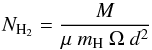 (2)where
mH is the mass of the hydrogen atom,
μ = 2.33 is the mean molecular mass in units of hydrogen atom masses,
and Ω the solid angle subtended by the dust continuum emission. Assuming the depth of
the region equals the projected one (i.e. 5000 AU), we derive an average density in the
range 0.9−2.6 × 107 cm-3 for OMC-2 FIR 4.
(2)where
mH is the mass of the hydrogen atom,
μ = 2.33 is the mean molecular mass in units of hydrogen atom masses,
and Ω the solid angle subtended by the dust continuum emission. Assuming the depth of
the region equals the projected one (i.e. 5000 AU), we derive an average density in the
range 0.9−2.6 × 107 cm-3 for OMC-2 FIR 4.
The channel maps in Fig. 4 reveal more details about the spatial distribution of the molecular line emission. Despite the low spectral resolution of the observations, the emission in all the tracers but DCO+(2–1) is detected above 5σ across five velocity channels (i.e. covering a width of about 18 km s-1), and therefore some kinematical information can already be extracted from these maps. We note, however, that in the case of DCN(2–1) this velocity spread is partly due to the hyperfine splitting (see Sect. 3.2.3 below). In Fig. 5 we show the average spectra within the main, west, and south sources, defined by the polygons shown in Fig. 3 (right panel). Figure 6 presents the first moment maps for the four molecular tracers observed with the PdBI (colour scale), with overlaying contours of the corresponding velocity-integrated maps. The spectra, channel maps, and velocity maps reflect the following properties:
-
The main source displays a velocity gradient in the south-west tonorth-east directions.
-
The west source as seen by CH3OH and C34S(3–2) appears slightly blue-shifted with respect to the systemic velocity of the source.
-
The DCO+(2–1) emission is significantly the narrowest in line width and concentrates almost exclusively on the south source.
-
A secondary, well-separated condensation is distinguished in the CH3OH and DCN(2–1) maps to the south-west of the main source, suggesting the presence of an additional physical source. The DCO+ emission also extends towards this area.
While the channel maps suggest the presence of more sources apart from the three we have identified so far, we cannot confirm it with 100% certainty at this spatial resolution, and even less guess how many more are present. We therefore conclude, as stated above, that there are at least three distinct sources within OMC-2 FIR 4, leaving open the possibility of further multiplicity within each of these three regions.
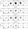 |
Fig. 4 Channel contour maps of each line detected with PdBI towards OMC-2 FIR 4. Contours start at 5σ and increase by steps of 5σ. The 1σ rms values are listed in Table 2. The velocity of each channel is marked on the top-left corner of each panel. Black crosses mark the phase centre of the observations, i.e. α(J2000) = 05h35m26.971s, δ(J2000) = –05°09′56.77″, while red crosses mark the positions of the three sources identified in this work (see Table 4). The bottom-left ellipses in each panel represent the beam sizes. |
3.2.2. Ammonia emission
The NH3(1, 1) and (2, 2) line spectra seen towards the peak NH3(1, 1) emission coordinates are shown in Fig. 7, with the different hyperfine components marked. The limited band width of the correlator allows us to cover only one pair of satellites for each transition, apart form the main component. In the case of NH3(2, 2), only the main component is detected.
Velocity-integrated ammonia maps are shown in Fig. 8, where the emission corresponds to the main hyperfine component of the NH3(1, 1) and NH3(2, 2) transitions. These are overlaid on the 2-mm continuum PdBI image for comparison. We stress that the presence of extended emission that was filtered out by the VLA results in a relatively high 1σ rms level in the clean maps. Indeed, Li et al. (2012) have recently published these ammonia data merged with single-dish maps obtained with the Green Bank Telescope (GBT), and a comparison with our VLA-only spectra indicates a flux loss of about 40%. Nevertheless, in terms of morphology, the NH3 emission is well defined around OMC-2 FIR 4 and peaks to the south of the main source. The emission appears extended, with a roundish shape, and covers an area which is larger than that of the 2-mm continuum.
 |
Fig. 5 Spectra in the three main sources identified in OMC-2 FIR 4 (see text) for each line tracer. The vertical scale is the brightness temperature of the line, TL, averaged across the area of the corresponding polygon (see Fig. 3). |
For completeness, in Fig. 9 we present the channel maps for the two NH3 transitions, with the velocity of the channels given in the top right-hand corner of each panel in km s-1. Unlike the millimetre molecular spectra (Sect. 3.2.1), the NH3 lines are rather narrow, as can be seen from the velocity range covered by the maps (see also the spectra in Fig. 7 and the FWHM values in Table 8). This may partly stem from the better spectral resolution and lower sensitivity of these observations. Indeed, the channel spacing of the VLA observations (~0.6 km s-1) is substantially smaller than that of the WIDEX PdBI spectra.
The channel maps show extended emission around the central coordinates of OMC-2 FIR 4, and several other sources of emission: two towards the north-east and the south-west, where FIR 3 and FIR 5 are located, respectively, and a third one towards the south-east at the systemic velocity of the source (11.4 km s-1), also seen in the single-dish 1.3-mm maps carried out by Chini et al. (1997).
3.2.3. Derivation of physical parameters
Both the DCN(2–1) and DCO+(2–1) lines are split into six hyperfine
components. For DCO+(2–1), all of them lie within a velocity range of 0.3 km
s-1, while for DCN(2–1) they span 8 km s-1. As a result, at the
spectral resolution of our observations, they are all blended and unresolved, so a
hyperfine analysis is not possible. We have thus performed a Gaussian fit to each line
and adopted a range of Tex between 10 and 100 K to estimate
a range of column densities from 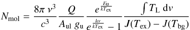 (3)where
ν, c, h, k,
Aul, τpeak,
ΔV, Q, gu,
Eup, and
(3)where
ν, c, h, k,
Aul, τpeak,
ΔV, Q, gu,
Eup, and  are, respectively, the
frequency of the transition, the speed of light, Planck constant, Boltzmann constant,
the spontaneous emission rate, the optical depth at the line intensity peak, the line
FWHM, the partition function, the upper state degeneracy, the upper level energy, and
the velocity-integrated line intensity. This equation assumes optically thin conditions,
and
are, respectively, the
frequency of the transition, the speed of light, Planck constant, Boltzmann constant,
the spontaneous emission rate, the optical depth at the line intensity peak, the line
FWHM, the partition function, the upper state degeneracy, the upper level energy, and
the velocity-integrated line intensity. This equation assumes optically thin conditions,
and  ,
with Tbg = 2.7 K. We applied the same approach to the
C34S(3–2) transition.
,
with Tbg = 2.7 K. We applied the same approach to the
C34S(3–2) transition.
The results of the Gaussian fits and the derived molecular column densities for each source are shown in Table 6, where it can be seen that we are indeed dealing with optically thin conditions. Some of the rows in this table probably correspond to “artificial” sources, since not all the sources we have identified are well-defined or traced by all the lines, as explained above. We nevertheless present them for comparison and completeness. The abundances of each molecule in the different sources are also listed. They have been obtained from the ratio of Nmol to the gas column density, N. For the latter, we have used the values listed in Table 5, adopting both Td = 20 K and Td = 50 K.
As for the methanol lines, we analysed them by means of a large velocity gradient (LVG) code, originally developed by Ceccarelli et al. (2003) and modified to include the methanol collisional coefficients with H2 by Pottage et al. (2004). For this analysis, we used the methanol lines obtained by averaging the emission over the entire OMC-2 FIR 4 clump. The line intensities thus measured are listed in Table 7, where the values shown for the 145-GHz lines do not correspond to single transitions but to ensembles of blended methanol lines around the indicated frequency and transition. We ran a large grid of models to cover a wide parameter space: N(CH3OH) from 1013 to 4 × 1015 cm-2, density from 104 to 109 cm-3 and temperature from 10 to 200 K. The observed lines were compared with the LVG model predictions and the best fit solution was found by minimising the χ2 value with respect to the three above parameters, assuming a source size of 15″ × 15″, as measured in our maps for the whole OMC-2 FIR 4 clump. We note that for the blended lines the predicted intensities were obtained by adding the intensity by each single line in the velocity interval.
We found that the CH3OH column density is very well constrained between 0.6 and 1 × 1015 cm-2, roughly consistent with the value of ~2 × 1014 cm-2 reported by Kama et al. (2010) from the early results of the HIFI data. The density is between 0.2 and 1 × 107 cm-3, a range of values that matches the average density we obtain from the millimetre continuum emission (see Sect. 3.2.1). The predicted optical depths of the CH3OH lines are low, around a few times 10-2.
The observed lines do not allow to constrain the temperature, except that it is higher than 20 K. The higher the CH3OH column density, the higher the gas temperature. For example, if N(CH3OH) is 8 × 1014 cm-2 then the gas temperature is higher than 50 K; for N(CH3OH) = 1 × 1015 cm-2 the gas temperature is higher than 120 K. More methanol transitions will be necessary to constrain the temperature better, but our analysis already shows that the gas emitting the methanol lines must be relatively dense. The best fit solutions of the LVG modelling have a reduced χ2 below 0.5 and are summarised in Table 7.
OMC-2 FIR 4 sources: Gaussian fit results, column densities and abundances for each PdBI tracer.
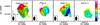 |
Fig. 6 Velocity maps (colour scale, in km s-1) of each line detected with PdBI towards OMC-2 FIR 4, with overlaying contours of the corresponding velocity-integrated maps. Contour levels are as in Fig. 3. The bottom-left ellipse in each panel represents the beam size. Crosses mark the phase centre of the observations, i.e. α(J2000) = 05h35m26.971s, δ(J2000) = –05°09′56.77″. |
Finally, we performed a hyperfine line fit to the two ammonia spectra in Fig. 7 using the standard NH3(1, 1) and NH3(2, 2) methods in CLASS. We subsequently derived the corresponding rotational and kinetic temperatures, as well as the NH3 column density, following the steps summarised in Busquet et al. (2009) and assuming a beam-filling factor equal to 1. The results are reported in Table 8, where the peak synthesised beam temperature, TSB, the velocity, VLSR, and the optical depth, τmain refer to the main component of the transition. We note that the errors on the temperature and column density estimates are close to or greater than the values themselves, mostly due to the large errors on TSB and τ. Using the H2 column densities listed in Table 5, we obtain an NH3 abundance that is slightly above 10-10. While this value is about two orders of magnitude less than what is typically reported in the literature, there are studies of ammonia in dense molecular cores that find values as low as ours or even lower (e.g. Foster et al. 2009; Wootten 1995).
4. Discussion
4.1. Source multiplicity within OMC-2 FIR 4
Several studies (Jørgensen et al. 2006, S08; Crimier et al. 2009; Kama et al. 2010) suggest that OMC-2 FIR 4 contains three main components:
-
a large-scale cool envelope about10 000 AU (i.e.0.05 pc) across,
-
an inner hot core, with kinetic temperatures above 100 K and around 400 AU in size,
-
a shock region produced by the interaction of an external bipolar outflow driven by the nearby OMC-2 FIR 3, which lies to the north-east of FIR 4.
In addition, S08 report the presence of 11 cores seen at 3-mm inside this region, and speculate that such fragmentation has been externally triggered by the FIR 3 outflow.
The emission of all the maps presented in Sect. 3 covers roughly 10 000 AU (0.05 pc) and therefore traces the envelope component of OMC-2 FIR 4. In particular, this component appears to be better traced by the NH3 maps, which are essentially single-peaked and display the most extended emission, similar in size and morphology to the structures detected in previous single-dish observations (e.g. Chini et al. 1997; the ASTE maps of Shimajiri et al. 2008). The temperature derived for the ammonia emission, ~30 K, is typical of protostellar (in our case protocluster) envelopes (e.g. Olmi et al. 2012).
At the resolution of our PdBI observations we cannot confirm the existence of the 11 cores claimed by S08, despite its being slightly better than that of the NMA observations. Inspection of the different maps presented in this work allows us to clearly separate three regions, denoted by the identifiers main, west, and south (Sect. 3.2.1). It appears, however, that our 2-mm continuum and some molecular line maps indeed hint at the presence of multiple smaller condensations within the three regions we detect, but these will need to be confirmed by higher angular resolution observations.
CH3OH line intensities and results of the LVG analysis.
At this point, it is worth mentioning that the hot-core hypothesis proposed by Crimier et al. (2009) is based on a single source at the centre of the large-scale envelope. S08 and our new observations show that the envelope component breaks down at scales of ~2000 AU, so much larger than the presumed hot core size (with a radius of 440 AU). Only high-angular resolution imaging of typical hot core tracers (e.g. complex organic molecules) can observationally prove the existence of a hot core.
As shown in Fig. 6, a velocity difference of about 6 km s-1 can be seen between the south-west and the north-east extremes of the main source in the CH3OH and C34S(3–2) maps, with the north-eastern tip being the most red-shifted. S08 find the same behaviour in their single-dish methanol maps. Additional interferometric observations of CO and SiO lines provided the same authors with morphological and dynamical evidence that led them to suggest that there is an interaction between the north-eastern edge of OMC-2 FIR 4 and the molecular outflow driven by the nearby FIR 3. The red-shifted emission we detect from CH3OH and C34S(3–2) may also be explained by this scenario; i.e., it arises from shocked gas from the interaction between the FIR 3 outflow and the dense gas of FIR 4. It might alternatively be tracing the FIR 3 outflow itself, which cannot be detected much beyond the boundary of the FIR 4 clump due to the limited sensitivity of the PdBI to more extended structures. More observations are needed to confirm the external outflow interpretation, since with our data alone we are not able to conclude that this is indeed the case. Other possibilities exist that could cause a velocity gradient like the one we detect, such as rotation or internal outflowing/expanding motions.
Results of the line fitting to the NH3(1, 1) and (2, 2) lines and derived physical parameters.
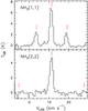 |
Fig. 7 VLA ammonia spectra obtained towards the peak coordinates of OMC-2 FIR 4, with a channel width of 0.62 km s-1. The different hyperfine components are marked with red vertical lines. |
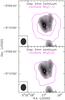 |
Fig. 8 Velocity-integrated VLA ammonia contour maps obtained towards OMC-2 FIR 4, overlaid on the naturally weighted 2 mm-continuum map (grey scale). Contours for all the maps start at 3σ and increase by steps of 3σ. The 1σ rms values are 20 mJy beam-1 km s-1 for both NH3(1, 1) and NH3(2, 2). White crosses mark the positions of the three sources identified in this work (see Table 4). |
4.2. Nature of the sources
Our observations allow us to distinguish three separate sources that may or may not present more substructure:
-
1.
The main source, at the nominal coordinates and systemicvelocity (11.4 km s-1) of OMC-2 FIR 4. It is the strongest 2-mm continuum and methanol source in the region. Its elongated shape suggests that it harbours two or more individual cores, although this hypothesis can only be confirmed with higher spatial resolution imaging. The red-shifted velocity of its northern portion might indicate an interaction with the red-shifted lobe of the external outflow driven by FIR 3.
-
2.
The west source, with a systemic velocity of 9–10 km s-1. It is well traced by C34S(3–2) and DCN(2–1), and weaker than the main source emission.
-
3.
The south source, also with VLSR = 9–10 km s-1, best traced by DCO+(2–1). It is the faintest methanol, DCN, and 2-mm continuum source, and has no significant emission in C34S(3–2). Its association with DCO+ indicates this region is likely colder than the other two, suggesting that it contains either a starless core or a protostar in an earlier evolutionary stage or with a lower mass (e.g. Jørgensen et al. 2004). Alternatively, since it does not display any emission peak in the 2-mm continuum image, it may not be a separated molecular core, but part of the cold external envelope of OMC-2 FIR 4.
From the results of our LVG analysis on the CH3OH lines, we find that the entire OMC-2 FIR 4 clump is rather dense (n > 2 × 106 cm-3 at 15″, i.e. 6000 AU). This suggests that the three regions we identify in this work, which are all together smaller in size when compared to the whole emission considered in the CH3OH analysis, may be even denser. We note that the density we derive is in good agreement with S08 and with the predictions made by Crimier et al. (2009), both of which report a value of 106 cm-3.
 |
Fig. 9 VLA NH3(1, 1) and NH3(2, 2) channel maps towards OMC-2 FIR 4. Contours start at 5σ and increase by steps of 5σ. The 1σ rms values are 5.0 mJy beam-1 for NH3(1, 1) and 4.7 mJy beam-1 for NH3(2, 2). The velocity of each channel is marked in the top-right corner of each panel in units of km s-1. Red crosses mark the positions of the three sources identified in this work (see Table 4). Green circles mark the position of FIR 3 (NE) and FIR 5 (SW) according to the 1.2 mm observations of Chini et al. (1997). The bottom-right ellipses in each panel represent the beam sizes. |
4.3. An ionised region in OMC-2 FIR 4
Radio-continuum observations of the OMC2/3 filament were carried out with the VLA by Reipurth et al. (1999) at 3.6 cm. At the position of OMC-2 FIR 4, they detected an elongated source that the authors interpret as a radio jet. When comparing their map with our PdBI map, despite the different angular resolutions (i.e. ~4′′ for the PdBI maps, 8″ for the VLA maps), we find that the position and shape of the radio source coincides fairly well within the pointing errors of the two maps, with the emission distribution of our 2-mm continuum and methanol PdBI images, which are both elongated in the same direction as the VLA source (see Fig. 10).
While Reipurth et al. (1999) attribute the radio continuum emission to a jet, the interferometric observations performed towards this source so far (e.g. S08, this work) have failed to detect molecular line emission at the high velocities indicative of a jet or outflow emanating from this region. This leads us to consider a different possibility, namely that the radio emission arises from a very compact gas cavity ionised by a central young star, i.e. an Hii region, which is either surrounded by a shell of dust and molecular gas best traced by the 2-mm continuum and CH3OH emission, or else harbours two or more unresolved molecular dense cores within it. The Hii region scenario is a plausible explanation for the continuum radio emission, since IM protostars can also produce sufficiently intense Hii regions to be easily detected at centimetre wavelengths (e.g. Thompson 1984).
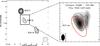 |
Fig. 10 Left panel: VLA map of the 3.6 cm continuum emission in the OMC-2 FIR 4 region and its surroundings (taken from Reipurth et al. 1999). The synthesised beam is shown at the bottom-right corner. The source labelled VLA 12 coincides with the position of OMC-2 FIR 4. Right panel: close-up view showing our PdBI continuum (grey scale) and CH3OH (black contours) maps. The synthesised beam is shown at the bottom-left corner. The red ellipse schematically represents the 4σ contour of the VLA image (left panel). The red cross marks the position of the cm emission peak. |
Reipurth et al. (1999) measured a flux of 0.64 mJy at 3.6 cm towards OMC-2 FIR 4. In the scenario of an optically thin Hii region, and assuming a single zero-age main sequence star is powering it, this implies a B3–B4 spectral type for the central star (using the tables of e.g. Panagia 1973; Thompson 1984; Martins et al. 2005). This translates into a luminosity between 700 and 1000 L⊙ and would indicate that this young star is the most massive source in the protocluster. It is also possible, given the elongated shape of the radio emission, that two (or more) individuals are responsible for the ionisation of their surroundings. Only higher angular resolution and sensitivity images of the continuum emission at different wavelengths will allow us to verify this possibility and find out whether the nature of the centimetre emission is an Hii region, as proposed here, or a radio jet.
4.4. A final note on luminosities
There is some confusion regarding the luminosity of OMC-2 FIR 4 in the literature. While the first estimates by Mezger et al. (1990), and later by Crimier et al. (2009), report a value between 400 L⊙ and 1000 L⊙, a recent work by Adams et al. (2012) yields 50 L⊙. In what follows we try to understand the reason for this discrepancy.
The first point to mention is the complexity of the region. Indeed, the morphology and size of OMC-2 FIR 4 change when seen at different wavelengths. In the mid-IR it appears to be a compact source, while at wavelengths above ~100 μm its emission is more extended (~30′′ in diameter) and peaks around 5″ west of the mid-IR source. This said, we note that the luminosity estimates published by the different authors refer to different components. On the one hand, Adams et al. (2012) built the SED of the source by measuring the continuum fluxes, at IR and sub-mm wavelengths, of the compact source they detect at 19 μm and 37 μm with SOFIA. In other words they adopted small aperture sizes, ranging between 7″ and 13″ and centred on the mid-IR peak. On the other hand, Crimier et al. (2009) and Mezger et al. (1990) took into larger areas into account, which are 30″ and 50″ in diameter, respectively, which include the whole envelope of OMC-2 FIR 4. In particular,
-
Crimier et al. (2009) used far-IRdata from ISO and IRAS, whose coarse angular resolution likelyled to measured fluxes that were overestimated, owing to possiblecontamination from the nearby protostar FIR 3, byat most a factor 2, since at such wavelengths thedominant emission source is FIR 4.
-
Adams et al. (2012) obtained Herschel-PACS maps of OMC-2 FIR 4 from which they measured the fluxes at 70 μm and 160 μm. They did so by applying small apertures of
 and
and
 , respectively, around the
mid-IR peak coordinates, and a background annulus that actually covers part of the
extended emission of the region. In addition, they carried out APEX observations at
350 μm and 850 μm that lacked the sensitivity
needed to detect any emission. They therefore measured an upper limit of the flux
considering only the emission within a beam size (7.3″ and 19″, respectively), again
around the mid-IR coordinates, and therefore offset by ~5″ from the actual sub-mm
peak position. As a result, their reported sub-mm fluxes are respectively ten and
three times lower than those detected and measured by Crimier et al. (2009) with the CSO and JCMT telescopes.
Considering these points, the authors may have underestimated the flux of OMC-2 FIR
4 by a factor of up to ten.
, respectively, around the
mid-IR peak coordinates, and a background annulus that actually covers part of the
extended emission of the region. In addition, they carried out APEX observations at
350 μm and 850 μm that lacked the sensitivity
needed to detect any emission. They therefore measured an upper limit of the flux
considering only the emission within a beam size (7.3″ and 19″, respectively), again
around the mid-IR coordinates, and therefore offset by ~5″ from the actual sub-mm
peak position. As a result, their reported sub-mm fluxes are respectively ten and
three times lower than those detected and measured by Crimier et al. (2009) with the CSO and JCMT telescopes.
Considering these points, the authors may have underestimated the flux of OMC-2 FIR
4 by a factor of up to ten.
In short, it appears that the discrepancy in luminosity estimates found in the literature is caused by the fact that different authors measure different components of OMC-2 FIR 4, with Adams et al. (2012) concentrating on the compact mid-IR source and Crimier et al. (2009) on the entire envelope, which is several times larger. Table 9 summarises the different values for the luminosity, mass, and size of OMC-2 FIR 4 reported in the literature. Based on the discussion above, the actual value depends on how one defines OMC-2 FIR 4 and its boundaries. If our interpretation of an Hii region is correct (see Sect. 4.3), the luminosity of the whole protocluster could be around several hundred solar luminosities.
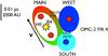 |
Fig. 11 Schematic cartoon of OMC-2 FIR 4 and the nearby OMC-2 FIR 3, summarising all the physical elements in the region that we propose according to the data presented in this work (see Sect. 4). The white ellipse inside the main source depicts the ionised region powered by a B4 young star. The colours of the main, west, and south sources represent their systemic velocities with respect to the nominal value for OMC-2 FIR 4 (VLSR = 11.4 km s-1), marked in green. The small red and blue circles within the three sources represent the possibility that they harbour smaller unresolved molecular condensations, with the colour blue denoting a colder temperature than red. |
5. Conclusions
We have presented new interferometric observations carried out towards the intermediate-mass protocluster OMC-2 FIR 4 in the Orion A complex. These include PdBI maps of the continuum emission at 143.4 GHz (2 mm) and the CH3OH(3, 1, +0 – 2, 1, +0), C34S(3–2), DCN(2–1), and DCO+(2–1) lines, as well as VLA maps of the NH3(1, 1) and (2, 2) inversion transitions. Despite the coarse channel spacing of the observations (0.6 km s-1 for the VLA spectra and 4 km s-1 for the PdBI images), we were able to extract important information about the morphology and kinematics of the region. Figure 11 shows a cartoon of the OMC-2 FIR 4/FIR 3 region, summarising all the elements present according to our interpretation of the data presented in this work. Our findings are summarised as follows.
-
1.
Our 2-mm continuum maps reveal two main components andhints of secondary cores or clumps surrounding it. The existenceof the 11 cores discovered by S08 could not beconfirmed by our observations, despite our higher angularresolution.
-
2.
Each PdBI line traces the region differently. By comparing their emission, we were able to distinguish three separate sources of one or several solar masses each, which we have named main, west, and south. The main and west ones are warmer. The south source displays a stronger line emission in DCO+(2−1), suggesting a colder temperature and therefore an earlier evolutionary state or lower mass core. Alternatively, it may be associatied with part of the colder envelope of OMC-2 FIR 4. As for the ammonia maps, their emission is more extended and essentially single-peaked, and therefore traces the envelope of the protocluster. An LVG modelling of the CH3OH lines we observed allowed us to conclude that the whole protocluster is very dense, with n ≳ 2 × 106 cm-3, in agreement with previous theoretical predictions on the structure of the envelope of OMC-2 FIR 4.
-
3.
The main source as seen by the 2-mm continuum and CH3OH emission coincides, both in position (within the pointing errors) and in shape, with the radio-continuum emission observed at 3.6 cm with the VLA (Reipurth et al. 1999). In the absence of clear interferometric evidence of a molecular outflow driven by FIR 4, we interpreted this as an Hii region powered either by a B3-B4 type young star or by two or more lower-mass stellar objects. This region is likely surrounded by a shell of dust and molecular gas (seen by the millimetre continuum and CH3OH maps). This scenario still needs to be verified by higher angular resolution and multi-wavelength observations.
Thanks to its relative proximity to the Sun, OMC-2 FIR 4 is an ideal laboratory to explore intermediate- and low-mass star formation in the context of a whole protocluster. The evidence of core multiplicity in this region, coupled with the insufficient spatial resolution of our observations to clearly separate them, highlights the need of higher spectral and angular resolution imaging to disentangle the different components and extract more information about the kinematics and the excitation conditions in each of them. This information will be crucial for interpreting the Herschel-HIFI data obtained towards this source within the CHESS key programme.
Herschel is a European Space Agency (ESA) space observatory with science instruments provided by European-led principal investigator consortia and with important participation from the National Aeronautics and Space Administration (NASA).
The GILDAS package is available at http://www.iram.fr/IRAMFR/GILDAS
The Very Large Array (VLA) is operated by the National Radio Astronomy Observatory (NRAO), a facility of the National Science Foundation operated under cooperative agreement by Associated Universities, Inc.
Acknowledgments
A.L.S. and C.C. acknowledge funding from the CNES (Centre National d’Études Spatiales) and from the Agence Nationale pour la Recherche (ANR), France (project FORCOMS, contracts ANR-08-BLAN-022). M.K. gratefully acknowledges funding from an NWO grant, NOVA, Leids Kerkhoven-Bosscha Fonds, and the COST Action on Astrochemistry. C.D. acknowledges funding from Leids Kerkhoven-Bosscha Fonds. A.F. has been partially supported within the programme CONSOLIDER INGENIO 2010, under grant CSD2009-00038 “Molecular Astrophysics: The Herschel andALMA Era – ASTROMOL”. We are grateful to the anonymous referee and to C.M. Walmsley, whose suggestions contributed to improve the quality of the present paper.
References
- Adams, J. D., Herter, T. L., Osorio, M., et al. 2012, ApJ, 749, L24 [NASA ADS] [CrossRef] [Google Scholar]
- Beuther, H., Churchwell, E. B., McKee, C. F., & Tan, J. C. 2007, in Protostars and Planets V, eds. B. Reipurth, D. Jewitt, & K. Keil, 165 [Google Scholar]
- Bottinelli, S. 2006, Ph.D. Thesis, University of Hawaii at Manoa [Google Scholar]
- Busquet, G., Palau, A., Estalella, R., et al. 2009, A&A, 506, 1183 [NASA ADS] [CrossRef] [EDP Sciences] [Google Scholar]
- Ceccarelli, C., Maret, S., Tielens, A. G. G. M., Castets, A., & Caux, E. 2003, A&A, 410, 587 [NASA ADS] [CrossRef] [EDP Sciences] [Google Scholar]
- Ceccarelli, C., Caselli, P., Herbst, E., Tielens, A. G. G. M., & Caux, E. 2007, in Protostars and Planets V, eds. B. Reipurth, D. Jewitt, & K. Keil, 47 [Google Scholar]
- Ceccarelli, C., Bacmann, A., Boogert, A., et al. 2010, A&A, 521, L22 [NASA ADS] [CrossRef] [EDP Sciences] [Google Scholar]
- Cesaroni, R., & Wilson, T. L. 1994, A&A, 281, 209 [NASA ADS] [Google Scholar]
- Chini, R., Reipurth, B., Ward-Thompson, D., et al. 1997, ApJ, 474, L135 [NASA ADS] [CrossRef] [Google Scholar]
- Crapsi, A., Caselli, P., Walmsley, C. M., et al. 2005, ApJ, 619, 379 [Google Scholar]
- Crimier, N., Ceccarelli, C., Lefloch, B., & Faure, A. 2009, A&A, 506, 1229 [NASA ADS] [CrossRef] [EDP Sciences] [Google Scholar]
- Crimier, N., Ceccarelli, C., Alonso-Albi, T., et al. 2010, A&A, 516, A102 [NASA ADS] [CrossRef] [EDP Sciences] [Google Scholar]
- de Graauw, Th., Helmich, F. P., Phillips, T. G., et al. 2010, A&A, 518, L6 [NASA ADS] [CrossRef] [EDP Sciences] [Google Scholar]
- Foster, J. B., Rosolowsky, E. W., Kauffmann, J., et al. 2009, ApJ, 696, 298 [NASA ADS] [CrossRef] [Google Scholar]
- Fuente, A., Ceccarelli, C., Neri, R., et al. 2007, A&A, 468, 37 [Google Scholar]
- Fuente, A., Castro-Carrizo, A., Alonso-Albi, T., et al. 2009, A&A, 507, 1475 [NASA ADS] [CrossRef] [EDP Sciences] [Google Scholar]
- Hildebrand, R. H. 1983, QJRAS, 24, 267 [NASA ADS] [Google Scholar]
- Johnstone, D., & Bally, J. 1999, ApJ, 510, L49 [NASA ADS] [CrossRef] [Google Scholar]
- Johnstone, D., Boonman, A. M. S., & van Dishoeck, E. F. 2003, A&A, 412, 157 [NASA ADS] [CrossRef] [EDP Sciences] [Google Scholar]
- Jørgensen, J. K., Schöier, F. L., & van Dishoeck, E. F. 2004, A&A, 416, 603 [NASA ADS] [CrossRef] [EDP Sciences] [Google Scholar]
- Jørgensen, J. K., Johnstone, D., van Dishoeck, E. F., & Doty, S. D. 2006, A&A, 449, 609 [NASA ADS] [CrossRef] [EDP Sciences] [Google Scholar]
- Kama, M., Dominik, C., Maret, S., et al. 2010, A&A, 521, A39 [NASA ADS] [CrossRef] [EDP Sciences] [Google Scholar]
- Kama, M., López-Sepulcre, A., Dominik, C., et al. 2013, A&A, submitted, DOI: 10.1051/0004-6361/201219431 [Google Scholar]
- Kim, M. K., Hirota, T., & Honma, M. 2008, PASJ, 60, 991 [NASA ADS] [CrossRef] [Google Scholar]
- Li, D., Kauffmann, J., Zhang, Q., & Chen, W. 2012, ApJ, 768, 5 [Google Scholar]
- Lis, D. C., Serabyn, E., & Keene, J. 1998, ApJ, 509, 299 [Google Scholar]
- Liu, Q., Yang, J., Sun, Y., & Xu, Y. 2011, RA&A, 11, 67 [Google Scholar]
- Martins, F., Schaerer, D., & Hillier, D. J. 2005, A&A, 436, 1049 [NASA ADS] [CrossRef] [EDP Sciences] [Google Scholar]
- Menten, K. M., Reid, M. J., Forbrich, J., & Brunthaler, A. 2007, A&A, 474, 515 [NASA ADS] [CrossRef] [EDP Sciences] [Google Scholar]
- Mezger, P. G., Wink, J. E., & Zylka, R. 1990, A&A, 228, 95 [NASA ADS] [Google Scholar]
- Nielbock, M., Chini, R., & Müller, S. A. H. 2003, A&A, 408, 245 [NASA ADS] [CrossRef] [EDP Sciences] [Google Scholar]
- Olmi, L., Angles-Alcazar, D., Elia, D., et al. 2013, A&A, 551, A111 [NASA ADS] [CrossRef] [EDP Sciences] [Google Scholar]
- Ossenkopf, V., & Henning, T. 1994, A&A, 291, 943 [NASA ADS] [Google Scholar]
- Palau, A., Sánchez-Monge, Á., Busquet, G., et al. 2010, A&A, 510, A5 [NASA ADS] [CrossRef] [EDP Sciences] [Google Scholar]
- Palau, A., Fuente, A., Girart, J. M., et al. 2011, ApJ, 743, 32 [NASA ADS] [CrossRef] [Google Scholar]
- Panagia, N. 1973, AJ, 78, 929 [NASA ADS] [CrossRef] [Google Scholar]
- Pottage, J. T., Flower, D. R., & Davis, S. L. 2004, MNRAS, 352, 39 [NASA ADS] [CrossRef] [Google Scholar]
- Reipurth, B., Rodríguez, L. F., & Chini, R. 1999, ApJ, 118, 983 [Google Scholar]
- Sánchez-Monge, Á., Palau, A., Estalella, R., et al. 2010, ApJ, 721, L107 [NASA ADS] [CrossRef] [Google Scholar]
- Shimajiri, Y., Takahashi, S., Takakuwa, S., Saito, M., & Kawabe, R. 2008, ApJ, 683, 255 [NASA ADS] [CrossRef] [Google Scholar]
- Shu, F. H., Adams, F. C., & Lizano, S. 1987, Ann. Rev. A&A, 25, 23 [NASA ADS] [CrossRef] [Google Scholar]
- Takahashi, S., Saito, M., & Ohashi, N. 2008, ApJ, 688, 344 [NASA ADS] [CrossRef] [Google Scholar]
- Tatematsu, K., Umemoto, T., & Kameya, O. 1993, ApJ, 404, 643 [NASA ADS] [CrossRef] [Google Scholar]
- Tatematsu, K., Kandori, R., Umemoto, T., & Sekimoto, Y. 2008, PASJ, 60, 407 [NASA ADS] [Google Scholar]
- Testi, L., Palla, F., & Natta, A. 1999, A&A, 342, 515 [NASA ADS] [Google Scholar]
- Thompson, R. I. 1984, ApJ, 283, 165 [NASA ADS] [CrossRef] [Google Scholar]
- van Kempen, T. A., Longmore, S. N., Johnstone, D., & Pillai, T. 2012, ApJ, 751, 137 [NASA ADS] [CrossRef] [Google Scholar]
- Williams, J. P., Blitz, L., & McKee, C. F. 2000, in Protostars and Plantes IV (Tucson: Univ. Arizona Press), 97 [Google Scholar]
- Wilner, D. J., & Welch, W. J. 1994, ApJ, 427, 898 [NASA ADS] [CrossRef] [Google Scholar]
- Wootten, A. 1995, Ap&SS, 224, 43 [NASA ADS] [CrossRef] [Google Scholar]
- Zinnecker, H., & Yorke, H. W. 2007, ARA&A, 45, 481 [NASA ADS] [CrossRef] [Google Scholar]
All Tables
OMC-2 FIR 4 sources: Gaussian fit results, column densities and abundances for each PdBI tracer.
Results of the line fitting to the NH3(1, 1) and (2, 2) lines and derived physical parameters.
All Figures
|
Fig. 1 Interferometric continuum maps of OMC-2 FIR 4 with natural (top) and uniform weighting (bottom). White contours represent the 2-mm continuum emission obtained with the PdBI, while black contours, as well as the background colour scale, correspond to the 3-mm continuum emission seen with the NMA (S08). Contours for both the PdBI and NMA maps start at 3σ and increase by steps of 3σ. The bottom-left ellipses represent the respective beam sizes. The white open circles mark the primary beam FWHM for the PdBI observations. The black crosses mark the NMA 3-mm cores as reported in Table 4 of S08. |
| In the text | |
|
Fig. 2 PdBI spectrum obtained towards the phase centre of OMC-2 FIR 4 with the WIDEX correlator. The species of the detected lines are labelled. |
| In the text | |
|
Fig. 3 Velocity-integrated PdBI contour maps obtained towards OMC-2 FIR 4, overlaid on the naturally weighted continuum map (grey scale). The bottom-left ellipse in each panel represents the beam size. Left: CH3OH(3, 1, +0 – 2, 1, +0) (black) and C34S(3–2) (magenta). Centre: DCN(2–1) (black) and DCO+(2–1) (magenta). All the contours start at 3σ and increase by steps of 3σ. The 1σ rms values are 0.16, 0.14, 0.17, and 0.08 Jy beam-1 km s-1, respectively for the CH3OH, C34S(3–2), DCN(2–1), and DCO+(2–1) integrated maps. Right: Polygons representing the three differentiated components, main, west, and south (see text), used to extract average spectra. The white crosses mark the positions of the three sources identified in this work (see Table 4). |
| In the text | |
|
Fig. 4 Channel contour maps of each line detected with PdBI towards OMC-2 FIR 4. Contours start at 5σ and increase by steps of 5σ. The 1σ rms values are listed in Table 2. The velocity of each channel is marked on the top-left corner of each panel. Black crosses mark the phase centre of the observations, i.e. α(J2000) = 05h35m26.971s, δ(J2000) = –05°09′56.77″, while red crosses mark the positions of the three sources identified in this work (see Table 4). The bottom-left ellipses in each panel represent the beam sizes. |
| In the text | |
|
Fig. 5 Spectra in the three main sources identified in OMC-2 FIR 4 (see text) for each line tracer. The vertical scale is the brightness temperature of the line, TL, averaged across the area of the corresponding polygon (see Fig. 3). |
| In the text | |
|
Fig. 6 Velocity maps (colour scale, in km s-1) of each line detected with PdBI towards OMC-2 FIR 4, with overlaying contours of the corresponding velocity-integrated maps. Contour levels are as in Fig. 3. The bottom-left ellipse in each panel represents the beam size. Crosses mark the phase centre of the observations, i.e. α(J2000) = 05h35m26.971s, δ(J2000) = –05°09′56.77″. |
| In the text | |
|
Fig. 7 VLA ammonia spectra obtained towards the peak coordinates of OMC-2 FIR 4, with a channel width of 0.62 km s-1. The different hyperfine components are marked with red vertical lines. |
| In the text | |
|
Fig. 8 Velocity-integrated VLA ammonia contour maps obtained towards OMC-2 FIR 4, overlaid on the naturally weighted 2 mm-continuum map (grey scale). Contours for all the maps start at 3σ and increase by steps of 3σ. The 1σ rms values are 20 mJy beam-1 km s-1 for both NH3(1, 1) and NH3(2, 2). White crosses mark the positions of the three sources identified in this work (see Table 4). |
| In the text | |
|
Fig. 9 VLA NH3(1, 1) and NH3(2, 2) channel maps towards OMC-2 FIR 4. Contours start at 5σ and increase by steps of 5σ. The 1σ rms values are 5.0 mJy beam-1 for NH3(1, 1) and 4.7 mJy beam-1 for NH3(2, 2). The velocity of each channel is marked in the top-right corner of each panel in units of km s-1. Red crosses mark the positions of the three sources identified in this work (see Table 4). Green circles mark the position of FIR 3 (NE) and FIR 5 (SW) according to the 1.2 mm observations of Chini et al. (1997). The bottom-right ellipses in each panel represent the beam sizes. |
| In the text | |
|
Fig. 10 Left panel: VLA map of the 3.6 cm continuum emission in the OMC-2 FIR 4 region and its surroundings (taken from Reipurth et al. 1999). The synthesised beam is shown at the bottom-right corner. The source labelled VLA 12 coincides with the position of OMC-2 FIR 4. Right panel: close-up view showing our PdBI continuum (grey scale) and CH3OH (black contours) maps. The synthesised beam is shown at the bottom-left corner. The red ellipse schematically represents the 4σ contour of the VLA image (left panel). The red cross marks the position of the cm emission peak. |
| In the text | |
|
Fig. 11 Schematic cartoon of OMC-2 FIR 4 and the nearby OMC-2 FIR 3, summarising all the physical elements in the region that we propose according to the data presented in this work (see Sect. 4). The white ellipse inside the main source depicts the ionised region powered by a B4 young star. The colours of the main, west, and south sources represent their systemic velocities with respect to the nominal value for OMC-2 FIR 4 (VLSR = 11.4 km s-1), marked in green. The small red and blue circles within the three sources represent the possibility that they harbour smaller unresolved molecular condensations, with the colour blue denoting a colder temperature than red. |
| In the text | |
Current usage metrics show cumulative count of Article Views (full-text article views including HTML views, PDF and ePub downloads, according to the available data) and Abstracts Views on Vision4Press platform.
Data correspond to usage on the plateform after 2015. The current usage metrics is available 48-96 hours after online publication and is updated daily on week days.
Initial download of the metrics may take a while.