© ESO, 2013

1. Introduction

Accretion discs are believed to drive the variability of supermassive black holes in active galactic nuclei (AGN) and, on much smaller time-scales, also the fluctuating signal from Galactic black holes in accreting compact binaries (Vio et al. 1992; Nowak et al. 1999; McHardy et al. 2006). Observed light curves, f  ≡  f(t), exhibit irregular, featureless variations at all frequencies that can be studied (Lawrence et al. 1987; McHardy & Czerny 1987; Gaskell et al. 2006). Nonetheless, accretion is the common agent (Frank et al. 2002).

Simplified models of accretion disc processes do not explain every aspect of variability of different sources. Phenomenological studies also show a considerable complexity of the structure of accretion flows. Accretion discs co-exist with their coronae and possibly winds and jets, which produce a highly unsteady contribution, and so the observed signal of the source is determined by the mutual interaction of different components (Done et al. 2007). In this paper we study X-ray variability features that can be attributed to stochastic flare events that are connected to the accretion disc. Our aim is to constrain the resulting variability using a very general scheme.

Random processes provide a suitable framework for a mathematical description of the measurements of a physical quantity that is subject to non-deterministic evolution, for example due to noise disturbances or because of the intrinsic nature of the underlying mechanism. In our previous paper (Pecháček et al. 2008, Paper I) we studied the theory of random processes as a tool for describing the fluctuating signal from accreting sources, such as AGN and Galactic black holes observed in X-rays. These objects exhibit a featureless variability on different time-scales, probably originating from an accretion disc surface and its corona. In particular, we explored a scenario where the expected signal is generated by an ensemble of spots randomly created on the accretion disc surface, orbiting with Keplerian velocity at each corresponding radius (Galeev et al. 1979; Czerny et al. 2004, and references therein).

Various characteristics can be constructed from the light curve of an astronomical object to study its variability properties (Feigelson & Babu 1992). The standard approach is to analyse the light curve in terms of its power spectral density (PSD), which provides the variability power as a function of frequency (Vaughan & Uttley 2008). The histogram of the flux distribution measures the time-scale that the source spends at a given flux level. Furthermore, the root-mean-square (rms) scatter can be computed for different sections of the light curve that correspond to different flux levels. This establishes the rms-flux relation (Uttley & McHardy 2001).

In this context an important reference to our work is given by Uttley et al. (2005), where the authors presented a model to explain the observed linear rms-flux relations that are derived from X-ray observations of accreting black hole systems. The model generates light curves from an exponential applied to a Gaussian noise, which by construction produces a log-normal flux distribution consistent with the observed X-ray flux histograms of the Galactic black hole binary Cyg-X1, as well as of other sources. Uttley et al. (2005) concluded that the observation of a log-normal flux distribution and the linear rms-flux relationship imply that the underlying variability process cannot be additive. Indeed, this statement holds for a large family of shot-noise variability models and it was extended to other sources in different spectral states (Arévalo & Uttley 2006), also in the optical band (Gandhi 2009).

As mentioned above, in this paper we concentrate on characteristics of the PSD profile, in particular on the constraints that can be derived from the PSD slope and the occurrence of break frequencies. Because power spectra do not provide complete information, even a perfect agreement between the predicted PSD and the data cannot be considered as a definitive confirmation of the scenario. We do not study additional constraints, such as the rms-flux relation or time lags between different bands, which certainly have a great potential of distinguishing between different schemes. Indeed, these characteristics provide complementary pieces of information that may be found incompatible with the spot model. In other words, the model presented here is testable, at least in principle, and it will be possible to confirm the model or reject it by observations.

Although well-known ambiguities are inherent to Fourier power spectra, an ongoing debate is held about the shape of the PSD and the dominant features that could reveal important information about the origin of the variability. The broad-band PSD has been widely employed to examine the fluctuating X-ray light curves, often showing a tendency towards flattening at low frequencies (Lawrence & Papadakis 1993; Mushotzky et al. 1993; Uttley et al. 2002). PSDs of interest for us are characterized by a power-law form of the Fourier power spectrum ωS(ω), which decays at the high-frequency part proportionally to the first power of ω. A break occurs at lower frequencies, where the slope of the power-law changes. The profile of the power spectrum can be even more complex, showing multiple breaks or even local peaks separated by minima of the PSD curve.

The occurrence of a break frequency has been discussed by various authors (e.g. Nowak et al. 1999; Markowitz et al. 2003) for its obvious relevance for understanding observed PSDs and interpreting the underlying mechanism that causes the slope change. In this context, McHardy et al. (2005) have examined the case of the Seyfert 1 galaxy MCG–6-30-15 with RXTE and XMM-Newton data. Very accurate fits suggest a multi-Lorentzian structure instead of a simple power-law. Furthermore, McHardy et al. (2007), combining the XMM-Newton, RXTE and ASCA observations, discovered multiple Lorentzian components in the X-ray timing properties extending over almost seven decades of frequency (10^-8 ≲ f ≲ 10^-2 Hz) of the narrow-line Seyfert 1 galaxy Ark 564. These authors concluded that the evidence points to two discrete, localized regions as the origin of most of the variability. Mushotzky et al. (2011) discussed the AGN optical light curves monitoring by Kepler. They found, rather surprisingly, that the PSD exhibits power-law slopes of − 2.6 to − 3.3, i.e., significantly steeper than typically seen in the X-rays. Furthermore, within the category of stellar-mass black holes, Pottschmidt et al. (2003) analysed Cygnus X-1 PSD from about three years of RXTE monitoring. These authors concluded that the changing form of the power spectrum can be interpreted as a combination of Lorentzians with gradually evolving amplitudes.

In this paper, motivated by this and similar observational evidence, we embark on a mathematical study of PSD that can be fitted either with a broken power-law or a double-bending power law, with the variability power ω S(ω) dropping at low and high frequencies, respectively. We consider a simplified (but still non-trivial) description of the intrinsic variability (random flares with idealized light curve profiles of the individual events), which allows us to develop an analytical approach to the resulting observable PSD profile. In particular, we determine conditions under which one, two, or more breaks or local maxima occur in the PSD. We calculate positions of these features and determine the changing slope of the model PSD.

The paper is organised as follows. In Sect. 2 we discuss the PSDs generated by a shot-noise-like random process with exponentially decaying flares. We developed a general approach to describe the morphology of the power spectra and demonstrate the results on a simple, analytically solvable example of a bi-Lorentzian PSD. In Sect. 4 we consider the influence of the modulation by the orbital motion on the PSDs. We summarise our conclusions and give perspectives for the application of this fast, analytical modelling scheme in Sect. 5.

2. Exponential flares

It is well known that the power spectra of stationary random processes must be flat at zero (S(ω) ∝ ω⁰) and integrable over all frequencies (i.e. decaying faster than ω^-1 for large ω). Moreover, it was demonstrated for the multi-flare model (Pecháček et al. 2008) that the high-frequency limit of the PSD is a power-law, S(ω) ∝ ω^γ, with the slope γ <  − 1 determined by the intrinsic shape of the flare-emission profile. The low frequency limit depends mainly on the statistics of the flare-generating process. The form of the intermediate part of the power spectrum is influenced by the interplay of all of these effects. The simplest possible power spectra generated by the flare model are approximately of the broken power-law form.

It is natural to assume that the power spectrum break-frequency is associated with some intrinsic time-scale of the process. This heuristic approach is supported by the basic scaling properties of the Fourier transform: rescaling the process in temporal domain by a factor a shifts the break frequency by a^-1. The power-law PSDs are invariant under this rescaling, and the break frequency is the only feature of the power spectra whose position changes. However, we will see that for two reasons it is difficult to go beyond this trivial observation.

Rigorous definition of the break frequency can be a problem. Even for the simplest acceptable feature-less power spectra such as a Lorentzian PSD, which are power-laws to high accuracy for most of frequencies, the change of slope occurs smoothly over a long interval. It is therefore not obvious which frequency should be defined as the break frequency, and even if we decide on some particular definition, various problems of interpretation may emerge.

In this introductory section, we constrain our discussion to mutually independent exponentially decaying flares with emissivity profiles I(t,τ) = I₀(τ)exp( − t / τ) θ(t), where θ(t) is the Heaviside function and τ is the lifetime of individual flares. Exponentials are well suited for our investigations because of their simple, feature-less power spectra. Moreover, there is a time-scale τ naturally and uniquely associated with each flare. This allows us to relate the break frequencies to the ensemble averages over the range of τ.

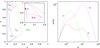Fig. 1 Left panel: diagram describing the morphology of the PSD profiles according to Eq. (4) for all possible values of the parameters α and K. Different curves represent the boundaries of subsets of the parameters for which the PSD exhibits a double-feature. The red curve encloses set CM of the doubly peaked power spectra. The other curves correspond to the sets of power spectra with a nontrivial structure of inflection points CI0 (blue), CI1 (magenta) and CIq (green). Right panel: three examples of the PSD profiles. A double-peaked power spectrum (red) with parameters α = 0.94 and K = 0.01 (i.e., the values within set CM, as denoted by the red point in the left panel), doubly-broken power spectrum with a single local maximum (magenta) corresponding to α = 0.85 and K = 0.08 (the magenta point within set CI1 and outside of CM) and a power spectrum with single maximum and break (green) with α = 0.5 and K = 0.5 (the green point outside of CIq).

Open with DEXTER

To simplify the problem even more, we do not take into account the relativistic effects in the rest of this section. The power spectrum of a random shot-noise-like process consisting of mutually independent exponentially decaying flares is given by (1)where λ is the mean rate of flares and p(τ) is the probability distribution of τ. In the case of identical emissivity profiles, i.e. with p_L(τ) = δ(τ − τ₀), the power spectrum is a pure Lorentzian, (2)Even this simple model can reproduce a wide variety of power spectra. In the context of the variability of the X-ray sources the model was introduced by Lehto (1989).

It is traditional to plot the PSDs in ω versus ωS(ω) graphs. It can be easily shown that the function ωS_L(ω) reaches its maximum at , as one can intuitively expect. In the general case the position of this maximum depends on the actual shape of the functions p(τ) and I₀(τ). Since the power spectrum is a nonlinear functional of the signal, the peak frequency differs from both E[τ]^-1 and , where E[.] denotes the averaging operator.

To demonstrate this nonlinear behaviour we will next study a process that consists of exponentials with only two different time-scales, i.e. a process with p(τ) = Aδ(τ − τ₁) + (1 − A)δ(τ − τ₂), where A is some constant from the interval ⟨ 0,1 ⟩ and τ₁ > τ₂. The resulting power spectrum is (3)As long as we are interested only in the process times-cales, the PSD normalization is irrelevant. Without loss of generality we can rescale the power spectrum both in normalization and in frequency domain as (4)Both K and α are from the interval ⟨ 0,1 ⟩. The peak frequency ω_M is given by the equation (5)which leads to the bicubical equation (6)where .

Fig. 2 Left: comparison of the time-scales τM (red) and E[τ] (magenta). The lines are calculated for α from the set {0.1, 0.2, 0.3, 0.4, 0.5, 0.6, 0.7, 0.8}, avoiding set CM. Middle: as in the left panel, but for α = 0.9. For low K this corresponds to double-peaked power spectra. The red curves correspond to 1 over the peak frequency, the green is for the minimum. The blue curve denotes the time-scale 1 / E[1 / τ]. Right: comparison of the time-scales τM (red) and 1 / E[1 / τ] (blue).

Open with DEXTER

Equation (6) can have either one or three positive real roots. For most of the combinations of parameters α and K the root is unique and the corresponding power spectrum has a single global maximum. Three roots do occur only for parameters within a small subset of the configuration space C_M. The corresponding power spectra have two local maxima separated by a local minimum. The boundary of set C_M is denoted by the red line in Fig. 1. Note that after rescaling the intrinsic time-scales of the two exponentials are 1 and K. The mean time-scale and the mean frequency of the process are then given by However, the break time-scale τ_M = 1 / ω_M depends nonlinearly on both α and K. The comparison of these three quantities is plotted in the Fig. 2. We can see that the displacement of the actual peak position and the two linearly averaged time-scales can be very significant.

Note that our formulae are expressed and graphs are labelled in arbitrary (dimensionless) units. When the underlying mechanism is interpreted in terms of flaring events in a black hole accretion disc, the meaning of these units can be identified with geometrical units. Corresponding quantities in physical units can be obtained by a simple conversion: 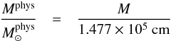(9)for the physical mass in grams, and 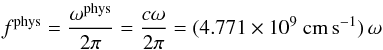(10)for the frequency in Hertz. Frequencies scale with the central mass proportionally to M^-1; their numerical values are therefore converted in the physical units by multiplying by the factor (11)For the black hole in Cyg X-1 the current mass estimate (Orosz et al. 2011) reads M^phys / M_⊙ = 14.8 ± 1.

From Figs. 1, 2 we learn that two peaks occur within only a very narrow parameter range. It is even more difficult to produce two peaks of similar height in the ω S(ω) plot. The condition is that two small numbers, K and 1 − α have to be equal. For example, in the hard state of Cyg X-1 the two most prominent Lorentzians are separated by about two decades in frequency, and they are of identical height, which means that in such a state K ≈ 0.01 and 1 − α = 0.01. Hence, the two quantities must be strongly correlated. Even if the two Lorentzians arise in different regions, the oscillations have to be physically linked. This mathematical statement is thus important and has to be taken into account in any attempt to explain the nature of the two mechanisms. Naturally, one has to bear in mind that all our conclusions are based on a simplified scenario; a more complicated (astrophysically realistic) model will very likely contain more parameters, which will bring additional degrees of freedom.

We have demonstrated that the power spectra S_r(ω) are double-peaked only for pairs of α and K within a small area of the parameter space. However, this does not mean that single-peaked power spectra are lacking any internal structure. Unlike the local maximum, it is not obvious how to formalize the presence of the internal structure into equations. The simplest continuation of the ideas above is to calculate inflection points of ωS(ω), (12)Apparently, Eq. (12) has also either one or three positive real solutions.

We have been investigating the local maxima of ωS(ω), because the power spectra S(ω) of a shot-noise-like processes are peaked at zero and because frequency times power versus frequency plots are traditionally used to analyse of astronomical signals. There is, however, no good a priori reason to prefer the inflection points of ωS(ω) over inflection points of S(ω) itself, 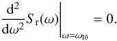(13)The regions C_I0 and C_I1 denote areas of the parameter space that exhibit more than one inflection point of S_r(ω), respectively ωS_r(ω). The critical points at their boundaries are connected by blue, and by magenta curve in the Fig. 1. These two areas clearly do not coincide, because the multiplication of the power spectra by ω can in some cases remove or create new inflection points. Inspired by the properties of the log–log plotting of power spectra, we can define the local power-law index of the PSD q(ω) and associate the internal structure of the power spectra with the presence of inflection points, 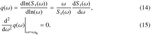The part of the parameter space corresponding to power spectra with more than one inflection point of q(ω) are within set C_Iq enclosed by the green curve in Fig. 1, which shows the positions of the inflection points of the three different types for a selected set of αs and a whole range of K.

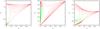	Fig. 3 Time-scales τI0 (left), τI1 (middle) and τIq (right) calculated for the PSD given by Eq. (4). We assumed the values of α from the set { 0.1, 0.2, 0.3, 0.4, 0.5, 0.6, 0.7, 0.8, 0.9 }, and K from the interval ⟨ 0,1 ⟩.
Open with DEXTER

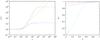	Fig. 4 Left: function g(x) (Eq. (19)) for the power spectrum (4), calculated for α = 0.95, and K = 0.01 (red) and K = 0.2 (blue), respectively. The green line represents the identity function g(x) = x. Right: the corresponding plot of time-scales, similar to the right panel of Fig. 2. The light-blue lines correspond to the limits from the inequality (21).
Open with DEXTER

2.1. A more general distribution of flare profiles

We now investigate a more general case with an arbitrary probability distribution p(τ). First we observe that the normalization function I₀(τ) has a similar influence on the resulting power spectrum as p(τ) itself. Therefore, we can without loss of generality study the power spectrum (16)where .

Without any loss of generality we can set λ =  [S(0)] ^-1. This rescaling does not change the overall shape of the PSD and it normalises to unity. Differentiating ωS(ω) from Eq. (16) leads to (17)For the peak frequency we find due to linearity of the averaging operator E [.], (18)Now we substitute x_M for , define a function g(x) as (19)and observe that the position of the local extreme is determined by the intersection of g(x) with x: 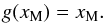(20)It follows from the Jensen inequality that the derivative of g is always non-negative (see the Appendix). Therefore, the position of x_M is constrained to the interval ⟨ g(0),g(∞) ⟩. Straightforwardly, . To calculate the upper limit we observe that 1 / (1 + τ²x) ∝ τ^-2 for τ² ≫ x^-1. Assuming that there is a non-zero lowest time-scale τ_min > 0 so that p(τ) = 0 for t < τ_min, we can replace the Lorentzian in (19) by τ^-2 and put¹. For the break time-scale we finally find the inequality (21)Figure 4 illustrates this again in terms of the power spectrum (4). Although g(x) is necessarily a non-decreasing function, the intersection g(x) = x needs not to be unique. The inequality (21) then holds for all local maxima and minima of the PSD.

We now further investigate properties of the function g(x). Equation (20) states that the extrema of the PSD are fixed points of g(x). We can define the nth iteration of g(x) by recurrent relations, (22)It trivially follows from Eq. (20) that the local extrema x_M are also fixed points of g⁽ⁿ⁾(x) for all values of n. Assuming distributions with finite moments g(0) and g(∞), the function g(x) maps the real half-line ⟨ 0,∞ ⟩ into the finite interval ⟨ g(0),g(∞) ⟩. From the monotonicity of g, it then follows that g maps the latter interval within itself.

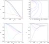Fig. 5 Top left: boundaries of approximating sets for the power spectrum Sr(ω). The function g(x) was evaluated in L points, evenly placed in between g(0) and g(∞). The nested curves correspond to calculated for L equal to 4, 5, 9, and 49. Top right: the nested sets calculated from the upper limit of g′(x). We have taken x+ = g(n)(0) and x− = g(n)(∞) for n from 1 to 4. Bottom left: the same as in the top left panel for sets . Bottom right: the same as in the bottom left panel, this time with a grid of points that samples the area around point 3h(0) more densely but that does not cover the whole interval ⟨ 3h(0),3h(∞) ⟩. The values of L are the same as in the previous examples. The approximating sets cover a broader part of the whole set . However, they omit a small area of high α. This demonstrates that an adaptive grid can perform significantly better than a regular one.

Open with DEXTER

By repeated applications of g we obtain an infinite sequence of nested inequalities, 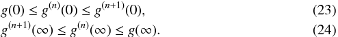Because of the Bolzano-Weierstrass theorem, the following limits exist and the same inequality holds for them as well, 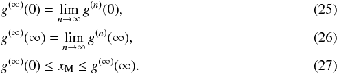Both g^(∞)(0) and g^(∞)(0) are fixed points of g(x) and correspond to the lowest and highest local maxima of ωS(ω), respectively. If they coincide, the power spectrum has a single peak.

The inflection points of the power spectrum can be investigated in a similar way. Defining a function (28)it can be easily proven that As we show in the Appendix, h(x) is also a non-decreasing function. Therefore, h(x) has properties similar to g(x), with h(0) = E [τ²]  / E [τ⁴], h(∞) = E [τ^-4]  / E [τ^-2] and with a similar structure of nested subintervals, (31)There are several applications of the previous relations. Clearly, finding the fixed points of g and h numerically is as hard as finding the extrema and inflection points of S(ω) directly. But by calculating g(0), h(0), g(∞) and h(∞), we can roughly estimate the position of each feature. Every application of these functions requires calculating two expected values of some functions of τ. It was demonstrated in the case of two Lorentzians that these limits are sometimes too wide. In this case we can always determine a tighter constraint by applying g and h, respectively, on the result at the cost of calculating two additional expected values per each iteration. Moreover, we can use g and h to find a constraint on the numbers of local extrema and inflection points.

In the simple case of two Lorentzians we were able to calculate directly for which subsets of the parameter space of α and K is the PSD doubly-peaked and doubly-broken. Let us call these sets C_M, C_I0, C_I1, and C_Iq. The parameter space of the general case with an arbitrary probability function is infinite-dimensional. In analogy with the two-dimensional case of S_r(ω) we can define a subsets of the space of all probability distribution functions , such that the power spectrum (16) has multiple local extrema x_M if, and only if, .

Testing if a particular function is contained in means calculating the power spectrum directly. However, using the function g(x), we can construct approximation sets and representing the necessary and sufficient conditions on to produce a multiply peaked power spectrum, . Using g and h, the approximating sets can be defined by an inequality, or a set of inequalities between some moments of τ. We now present two examples of such constructions and apply them to the example of the PSD (4).

2.2. Examples of the construction procedure

We take x₊ and x₋ such that x₊ < x_M < x₋ for all fixed points g(x_M) = x_M. By construction, g(x₊) > x₊ and g(x₋) < x₋. If there is more than one fixed point x_M, the function s_g(x) = g(x) − x changes its sign in the interval ⟨ x₊,x₋ ⟩ more than once. We can pick L values x_j from the interval such that x₊ < x₁ < ··· < x_L < x₋. If the sequence of s_g(x_j) changes sign more than once, the fixed point is not unique. Figure 5 shows the application of the test on the power spectrum (4) for x₊ = g(0), x₋ = g(∞) and x_j placed uniformly over the whole interval. The results are plotted for L equal to 4, 5, 9 and 50. Note that this is not the only possible choice of the x. All x₊ = g⁽ⁿ⁾(0) and x₋ = g⁽ⁿ⁾(∞) are admissible, and likewise, x_j can be chosen in some irregular or even adaptive way by using first L steps of some numerical root-finding method (e.g. the regula falsi method). What matters is the final complexity of the test. It produces a set of L inequalities that must be satisfied by to be in .

For set we can use a different approach. The well-known Banach fixed-point theorem says that if the function g is a contracting mapping, i.e. if there exists a number 0 ≤ λ < 1 such that | g(x) − g(y) |  < λ | x − y | for all admissible x and y, then the fixed-point x_M is unique. Because g(x) is a continuous and non-decreasing function, it follows from the mean value theorem that it is a contracting mapping if the maximum of its derivative is lower than one, g′(x) < 1. Defining a new function ℓ(x) as (32)we can write the derivative of g, 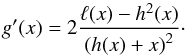(33)Similarly to g and h, also ℓ(x) is a non-decreasing function that can be expressed in terms of the functions g and h, (34)Because the function g maps the whole semi-axis ⟨ 0,∞ ⟩ into ⟨ g(0),g(∞) ⟩ it is sufficient to investigate the derivative g′(x) only on the latter interval. Because g, h, and ℓ are non-decreasing functions, the following inequality holds for all x₊, x₋ and y that satisfy g(0) ≤ x₊ ≤ y ≤ x₋ ≤ g(∞), (35)Using this inequality, we can take for the set of all distributions for which D_max(x₊,x₋) > 1. Figure 5 demonstrates this on the bi-Lorentzian power spectrum. We employed x₊ = g⁽ⁿ⁾(0) and x₋ = g⁽ⁿ⁾(∞) with n from 1 to 4. The margins derived from this criterion can be relatively wide, both because D_max(x₊,x₋) overestimates the maximum of g′(x), and also because some functions g(x) can have a single fixed point x_M and a derivative g′(y) > 1 (y ≠ x_M) at the same time. On the other hand, if D_max(x₊,x₋) < 1, g(x) surely exhibits a single fixed point.

Unfortunately, the analysis of inflection points of the local power-law slope cannot be generalized in the same way. However, we note that q(ω) is related to g by(36)From here we can immediately find that q(0) = 0 and q(∞) =  − 2. Furthermore, from (20) we see that q(ω_M) =  − 1 and conversely, by expressing g in terms of q, we can see that all ω with q(ω) =  − 1 are the fixed points of g. This is not surprising since in the vicinity of the local extreme (ω_M + y)S(ω_M + y) = const. + o(y). It is, however, a good motivation to briefly investigate the behaviour of the function ω^γS(ω) in terms of its local extrema ω_Mγ and inflection-points ω_Iγ, (37)Following the same procedure that led to the equations for x_M, x_I0, and x_I0, we obtain where A_γ = (γ − 2)(γ − 3), B_γ = 2(γ² − 3γ − 1) and C_γ = γ(γ − 1). We see that the solution of the problem is fully determined by the functions g and h.

This generalization brings nothing new for the local extrema x_Mγ. The constraints for the number of fixed points x_Mγ and methods for approximating their positions can be obtained from the corresponding methods for γ = 1 by replacing g(x) with g_γ(x) = γ(2 − γ)^-1g(x) and the local slope at the extremal points is q(ω_Mγ) =  − γ, as expected. However, the problem of the inflection points is more complicated with the exceptions of γ = 0 and γ = 1. A possible generalization of h(x) for γ ∈  ⟨ 0,1 ⟩ is given by (40)

3. Polynomial flares

In all of the previous considerations, we have assumed that the flare profiles are given by decaying exponentials and the distribution is positive and can be normalized to one. No other assumptions on were imposed. Therefore, the resulting inequalities are very general. We now approach the case of flares of the form (41)where P_k is a polynomial of kth order, and I₀(τ) is an arbitrary non-negative and quadratically integrable function. As a motivation we took I₀(τ) = 1 / τ, k = 1 and P₁(t / τ) = t / τ and calculated a power spectrum of a mixture of these profiles with the probability distribution p(τ), (42)It can be easily proven that the term S(ω | τ) from the previous equation satisfies a relation (43)Using this relation, we can rewrite Eq. (42) by integration by parts, (44)We observe that the power spectrum can be rewritten in the form If p(τ_min) = 0 and p(τ) − τp′(τ) ≥ 0 for all τ ∈  ⟨ τ_min,τ_max ⟩, p₂(τ) is behaving well, can be normalized to unity, and the power spectrum can be studied in terms of the functions g and h, as described previously, with the only difference that all averages must be calculated using p₂(τ) instead of p(τ).

It is not apparent on first sight how to interpret these average values. Therefore, we now study the general case of an arbitrary polynomial (42) assuming that the power spectrum can be reduced to the pure-exponential case. The PSD of a single profile (42) can be written as 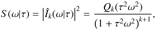(47)where Q_k(z) is a kth order polynomial, different than (but related to) P_k(t). We define by 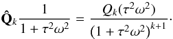(48)The operator is constructed entirely from τ, derivatives over τ, and from the coefficients of P_k (see the Appendix).

The generalization of Eq. (44) is 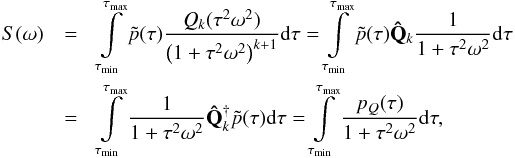(49)where is the Hermitian conjugate of . For p_Q(τ) positive over the interval of all admissible τs, we can calculate the function g(x), (50)where E_Q[.] is an averaging operator with respect to the distribution p_Q(τ). We note that we do not have to compute the function p_Q(τ).

As operates with τ only, it also commutes with the derivative in ω. Therefore, we can easily calculate the numerator and denominator of (50), 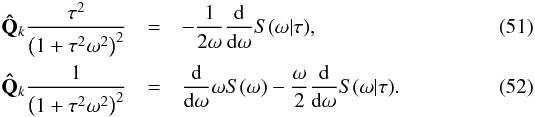The value of g(0) is related to the mean moment profiles as The function E_I(τ) can be interpreted as the total energy emitted by the flare and W_I(τ) is a measure of the width of the flare in the temporal domain. Equation (55) is formally identical with the prescription for the standard deviation. For the high-frequency limit we find (56)where q_l are the coefficients of the polynomial . The situation of h(x) is completely analogical. We can use the commutation properties of and express h(ω²) as (57)The asymptotic slope of the power spectra S(ω | τ) is q(∞) =  − 2(l + 1), where l is the order of the lowest non-zero coefficient of the polynomial P_k(t). Apparently, such a case can not be transformed onto the purely exponential case, because its asymptotical slope (36) is always q(∞) =  − 2. However, we can easily repeat the whole analysis for flares of the form I(t,τ) = (t^k / τ^k + 1)exp( − t / τ) θ(t), leading to the power spectrum (58)For every k we can define the functions g_k and h_k, It is easy to prove by direct calculation that the extrema and inflection points of ωS_k(ω) and S_k(ω) satisfy the relations 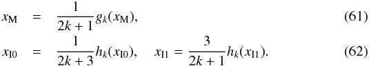Both g_k and h_k are non-decreasing (see the Appendix) and can therefore be used analogously to g and h. Apparently, g_k(0) = g(0) and h_k(0) = h(0), for the upper limits we find, (63)Finally, the local slope of S_k(ω) is related to g_k(x) by the formula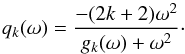(64)

3.1. Alternative forms of the function g

In the previous sections we described the properties of the function g. By construction, g-values are in every point directly related to the power spectrum and its derivatives; see Eqs. (36) and (50)–(52). However, in all previous applications we have required only that g is a non-decreasing function, g(0) and g(∞) are positive finite numbers, and its fixed points g(x_M) = x_M correspond to the local extrema of ωS(ω). Clearly, for given S(ω), these conditions do not fix the function uniquely. For instance, every member of the sequence g⁽ⁿ⁾(x) has the required properties. It is therefore natural to ask whether there is an alternative, easily calculable form of g.

A simple set of solutions to this problem can be found by adding a zero to Eq. (17) to obtain (65)where f(ω² | τ) is a function of ω² and τ. Properties of f(ω² | τ) are specified below. Due to linearity of the averaging operator we can define a new function g_[f](x) as (66)By construction, the functions g_[f](x) and g(x) have identical fixed points irrespective of the choice of f(x | τ). The limits of are given by where φ(τ) is the limit (69)Both f(0 | τ) and φ(τ) must be finite and chosen such that 0 < g_[f](0) ≤ g_[f](∞) < ∞. Unlike the previous cases, the positivity of the derivative of does not follow from any theorem and must be checked separately for every particular choice of f.

	Fig. 6 Left: boundary of set CM of doubly-peaked power spectra ωSrD(ω). Right: time-scales τM calculated for β from the set { 0.1, 0.2, 0.3, 0.4, 0.5, 0.6, 0.7, 0.8, 0.9 } and for Ωs from the interval ⟨ 0,10 ⟩. The blue line corresponds to . Again, the red lines denote the τM of the peaks, and the green lines denote the local minimum.
Open with DEXTER

4. Exponential flares with periodic modulation

In analogy with the previous section, we start the investigation with the simplest case of identical exponential flares modulated by sine function, (70)Without loss of generality we can put τ = 1 and rescale the power spectrum to the form (71)where β is taken from the interval ⟨ 0,1 ⟩. Figure 6 shows the boundary of set of the doubly peaked ω S_rD(ω) in the parameter space and the break time-scales τ_M for some choices of β and Ω_s. The structure of the set C_M corresponds again to the cusp catastrophe. However, the structure of inflection points, shown in Fig. 7, is more rich.

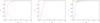Fig. 7 Left panel: boundary of the set CI0 (red) for the PSD (71). Parameters inside this area lead to PSD with a more than one inflection point. Unlike the power spectrum (4) SrD(ω) can have a global maximum at ω ≈ Ωs. CI1 (middle) and CIq (right) show the internal structure of the set. The common feature of the three panels are the critical curves (shown by other colours), where the number of inflection points changes.

Open with DEXTER

Unmodulated PSDs of the form (16) always satisfy the conditions S′′(ω) > 0 for ω → ∞ and S′′(0) =  − 2E [τ²]  < 0, and hence they have an odd number of inflection points. However, the power spectrum (71) can be convex both at zero and in the limit of high frequencies and therefore it can have an even number of inflection points. These two cases are separated by a curve β_crit(Ω_s) given by the condition . By direct calculation we find 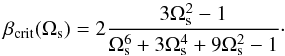(72)

4.1. General periodic modulation

We assumed that the exponentially decaying flares are at the same time orbiting in the equatorial plane of an accretion disc and that the observed signal is periodically modulated by the Doppler effect and abberation. It has been shown (Paper I) that the resulting power spectrum is described by the formula (73)where Ω(r) is the Keplerian orbital frequency, c_n(r) are the Fourier coefficients of the periodic modulation, and p(τ,r) is the probability density of finding a flare with the lifetime τ at the radius r. The formula (73) is far too complicated for calculations. Apparently, the factor can be again absorbed into the probability distribution. Integration over r and summation over n can be transformed into a single integral by appropriate change of the variables, r → Ω(r) / n. Finally, we can rewrite the Eq. (73) as (74)The function contains contributions from all harmonics of the orbital frequencies Ω(r) and is by construction symmetrical in the second variable . The distribution (75)leads to the PSD (71).

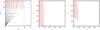Fig. 8 Left panel: graph of versus calculated for the PSD from Eq. (4). The deformed grid of contour lines corresponds to curves of α = const. and K = const. in the parameter space of the model, where ω∞ ≥ ω0 by construction. It follows that the image of the entire parameter space lies above the green diagonal line of ω∞ = ω0. Middle panel: the upper-left rectangular sector of acceptable pairs of ω0 and ω∞ from the left panel is projected back onto the (α,K) parameter space. Assuming the first-order boundaries of and , the pairs of α vs. K outside of the filled (red) area lead to the power spectrum, which can not have any local extrema at ωM. These parameter values are therefore ruled out. Right panel: analogical to the middle panel, but employing tighter (second-order) boundaries and ; in this case, the parameter constraints are more stringent (the filled area is smaller).

Open with DEXTER

We now repeat the procedures which, applied to Eq. (16), led to the definition of the functions g and h. We begin with the local extrema of ωS(ω). By differentiating (74), we find (76)The term 1 + τ²Ω² is always positive. Therefore, we can in analogy to Eq. (19) define the function g_Ω(x) as (77)and observe that the position of the local extrema is again given by the fixed point (78)The function g_Ω is positive and both g_Ω(0) and g_Ω(∞) are finite. Unfortunately, in a general case, g_Ω(x) is not a non-decreasing function. To be able to use the techniques developed in Sect. 2 we have to define a perturbed version of g_Ω(x) analogical to (66) as (79)where L(ω | τ,Ω) = ⁽1 + τ²(ω − Ω)^2)-1 is the elementary Lorentzian term. The perturbation f(ω² | τ,Ω) has to be finite at ω = 0 and to decay faster than ω^-1 to ensure the finiteness of g_[f]Ω(0) and g_[f]Ω(∞). Again, the positivity of the derivative of has to be tested for every particular choice f. For the power spectrum (71) it can be shown that (80)leads to a non-decreasing and positive function g_[f]Ω(ω²).

A general calculation of the points of inflection is even more problematic. One can proceed in the following way. Analogically to Eqs. (39) and (40), the function h_Ω(ω) is given by the solution of the following equations: The positivity of the derivative of h_Ω has to be ensured by the perturbation procedure.

5. Discussion and conclusions

We have described a general formalism that can be used to characterize the overall form of a power spectrum, namely, we determined the constraints on the functional form of the PSD shape that follow from the occurrence of local peaks. In particular, our approach allowed us to distinguish between PSDs that have the form of multiple power-law profiles with different numbers of local maxima. Our methodology is useful in the context of non-monotonic PSD profiles. In fact, Figs. 1 and 2 demonstrate that the occurrence of separate peaks of the PSD can put tight constraints on the model. The correct interpretation of these strict constraints still remains to be found. Naturally, a possible line of interpretation suggests that the spot/flare scenario is not generic and needs some kind of fine-tuning of the model parameters to reproduce observations. However, this calls for a more thorough investigation; in the present paper we only explored a highly idealized scheme in which strong assumptions were imposed. More complicated models (for instance, involving avalanches) also exhibit a more varied behaviour.

A potential application of our approach is illustrated in Fig. 8, where we constructed a mesh of two-dimensional contour-lines in a (α,K) parameter space of the model. Assuming that the exemplary power spectrum has a local maximum (or minimum) at frequency ω_M, it follows directly from Eq. (27) that the three frequencies must satisfy the relation ω₀ ≤ ω_M ≤ ω_∞. Only the parameters pairs α and K whose images are within the upper-left sector (Fig. 8, left panel), as described by the inequality, can produce a power spectrum with the required feature at ω = ω_M.

An example for this is Cyg X-1, which has been described as a superposition of several Lorentzians in the X-ray band light curve (Pottschmidt et al. 2003). These authors have demonstrated that the change of the timing parameters of the source is mainly caused by a strong decrease in the amplitude of one of the Lorentzian components present in the PSD. This characteristic is closely connected with the normalization of the model components. During the state transition of the source one of the Lorentzians becomes suppressed relative to the other. It was suggested that this behaviour is associated with the accretion disc corona, which is believed to be responsible for the hard-state spectrum. The evolution of the PSD form can be studied in terms of our method, which allowed us to discuss the entire class of multiple-power-law PSDs within a uniform systematic scheme. Although it is a versatile approach, its practical use can be illustrated in a very simple way.

The hard-state X-ray spectrum is very likely related with the presence of soft photons from the accretion disc, which are Compton up-scattered in a hot electron gas. The state transitions are then caused by the disappearance of the Comptonizing medium. Such a change in the coronal configuration could explain the change of the mutual normalization of the Lorentzian components, namely, the disappearance or recurrence of local peaks in the PSD. In the idea of coronal flares modulating the accretion disc variability of the source, which seems to be relevant for Cyg X-1 as well, the position of the source in Fig. 8 will constrain possible parameter values of the model.

Finally, we have checked that a certain proportionality between the light curve rms and the flux does exist in our model as well. This is an interesting fact by itself, however, it is not clear at present whether the slope and the scatter of the rms-flux relation are in reasonable agreement with the actual data, and how generic the model is. More detailed investigations are needed to clarify whether the spot model could satisfy the constraints arising beyond the PSD profiles. Moreover, it remains to be seen if our model requires some kind of special fine-tuning of the parameters (such as the inclination angle), which would make this explanation less likely (work in progress).

Acknowledgments

The research leading to these results has received funding from the Czech Science Foundation and Deutsche Forschungsgemeinschaft collaboration project (VK, GACR-DFG 13-00070J). We also acknowledge the Polish grant NN 203 380136 (B.C.) and the French GdR PCHE (R.G.). Part of the work was supported by the European Union Seventh Framework Programme under the grant agreement No. 312789 (M.D., B.C., R.G.). The Astronomical Institute has been operated under the program RVO:67985815 in the Czech Republic (TP).

References

Appendix A: Monotonicity of the functions g and h

We prove that the derivatives of g_k(x) and h_k(x) are non-negative. We define an operator F_x,k [.] by its action on an arbitrary function f(τ) as (A.1)where N_x,k is a normalization constant ensuring that F_x,k [1]  = 1 for all k and x. For a fixed value of x it acts as an mean value operator with a probability distribution p_x(τ) = p(τ) / ⁽1 + τ²ω^{2)− k − 3}. Using this operator, we can express the derivatives as The denominators in both equations are always non-negative. Furthermore, non-negativity of the numerator of (A.2) follows from the Jenssen theorem. The numerator of (A.3) is a determinant of a matrix of the following quadratic form: (A.4)Because the form is positively (semi-)definite, the determinant must be a non-negative function.

Appendix B: Operator associated with the polynomial Q

We give an explicit formula for the operator . We define operators and as (B.1)It can be proven by direct calculation that From these relations it follows, for arbitrary l and m, 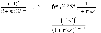(B.4)Assuming that , we can define the operator as 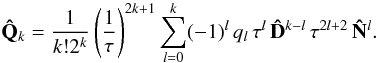(B.5)The polynomials Q_k and P_k are mutually related by the formula 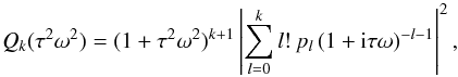(B.6)where p_l are the coefficients of P_k.

All Figures

	Fig. 1 Left panel: diagram describing the morphology of the PSD profiles according to Eq. (4) for all possible values of the parameters α and K. Different curves represent the boundaries of subsets of the parameters for which the PSD exhibits a double-feature. The red curve encloses set CM of the doubly peaked power spectra. The other curves correspond to the sets of power spectra with a nontrivial structure of inflection points CI0 (blue), CI1 (magenta) and CIq (green). Right panel: three examples of the PSD profiles. A double-peaked power spectrum (red) with parameters α = 0.94 and K = 0.01 (i.e., the values within set CM, as denoted by the red point in the left panel), doubly-broken power spectrum with a single local maximum (magenta) corresponding to α = 0.85 and K = 0.08 (the magenta point within set CI1 and outside of CM) and a power spectrum with single maximum and break (green) with α = 0.5 and K = 0.5 (the green point outside of CIq).
Open with DEXTER
In the text

	Fig. 2 Left: comparison of the time-scales τM (red) and E[τ] (magenta). The lines are calculated for α from the set {0.1, 0.2, 0.3, 0.4, 0.5, 0.6, 0.7, 0.8}, avoiding set CM. Middle: as in the left panel, but for α = 0.9. For low K this corresponds to double-peaked power spectra. The red curves correspond to 1 over the peak frequency, the green is for the minimum. The blue curve denotes the time-scale 1 / E[1 / τ]. Right: comparison of the time-scales τM (red) and 1 / E[1 / τ] (blue).
Open with DEXTER
In the text

	Fig. 3 Time-scales τI0 (left), τI1 (middle) and τIq (right) calculated for the PSD given by Eq. (4). We assumed the values of α from the set { 0.1, 0.2, 0.3, 0.4, 0.5, 0.6, 0.7, 0.8, 0.9 }, and K from the interval ⟨ 0,1 ⟩.
Open with DEXTER
In the text

	Fig. 4 Left: function g(x) (Eq. (19)) for the power spectrum (4), calculated for α = 0.95, and K = 0.01 (red) and K = 0.2 (blue), respectively. The green line represents the identity function g(x) = x. Right: the corresponding plot of time-scales, similar to the right panel of Fig. 2. The light-blue lines correspond to the limits from the inequality (21).
Open with DEXTER
In the text

	Fig. 5 Top left: boundaries of approximating sets for the power spectrum Sr(ω). The function g(x) was evaluated in L points, evenly placed in between g(0) and g(∞). The nested curves correspond to calculated for L equal to 4, 5, 9, and 49. Top right: the nested sets calculated from the upper limit of g′(x). We have taken x+ = g(n)(0) and x− = g(n)(∞) for n from 1 to 4. Bottom left: the same as in the top left panel for sets . Bottom right: the same as in the bottom left panel, this time with a grid of points that samples the area around point 3h(0) more densely but that does not cover the whole interval ⟨ 3h(0),3h(∞) ⟩. The values of L are the same as in the previous examples. The approximating sets cover a broader part of the whole set . However, they omit a small area of high α. This demonstrates that an adaptive grid can perform significantly better than a regular one.
Open with DEXTER
In the text

	Fig. 6 Left: boundary of set CM of doubly-peaked power spectra ωSrD(ω). Right: time-scales τM calculated for β from the set { 0.1, 0.2, 0.3, 0.4, 0.5, 0.6, 0.7, 0.8, 0.9 } and for Ωs from the interval ⟨ 0,10 ⟩. The blue line corresponds to . Again, the red lines denote the τM of the peaks, and the green lines denote the local minimum.
Open with DEXTER
In the text

	Fig. 7 Left panel: boundary of the set CI0 (red) for the PSD (71). Parameters inside this area lead to PSD with a more than one inflection point. Unlike the power spectrum (4) SrD(ω) can have a global maximum at ω ≈ Ωs. CI1 (middle) and CIq (right) show the internal structure of the set. The common feature of the three panels are the critical curves (shown by other colours), where the number of inflection points changes.
Open with DEXTER
In the text

	Fig. 8 Left panel: graph of versus calculated for the PSD from Eq. (4). The deformed grid of contour lines corresponds to curves of α = const. and K = const. in the parameter space of the model, where ω∞ ≥ ω0 by construction. It follows that the image of the entire parameter space lies above the green diagonal line of ω∞ = ω0. Middle panel: the upper-left rectangular sector of acceptable pairs of ω0 and ω∞ from the left panel is projected back onto the (α,K) parameter space. Assuming the first-order boundaries of and , the pairs of α vs. K outside of the filled (red) area lead to the power spectrum, which can not have any local extrema at ωM. These parameter values are therefore ruled out. Right panel: analogical to the middle panel, but employing tighter (second-order) boundaries and ; in this case, the parameter constraints are more stringent (the filled area is smaller).
Open with DEXTER
In the text

References

- Arévalo, P., & Uttley, P. 2006, MNRAS, 367, 801 [NASA ADS] [CrossRef] [Google Scholar]
- Czerny, B., Różańska, A., Dovčiak, M., Karas, V., & Dumont, A.-M. 2004, A&A, 420, 1 [NASA ADS] [CrossRef] [EDP Sciences] [Google Scholar]
- Done, C., Gierliński, M., & Kubota, A. 2007, A&ARv, 15, 1 [NASA ADS] [CrossRef] [EDP Sciences] [Google Scholar]
- Feigelson, E. D., & Babu, G. J. 1992, Statistical Challenges in Modern Astronomy (Berlin: Springer) [Google Scholar]
- Frank, J., King, A., & Raine, D. J. 2002, Accretion Power in Astrophysics (Cambridge: Cambridge University Press) [Google Scholar]
- Galeev, A. A., Rosner, R., & Vaiana, G. S. 1979, ApJ, 229, 318 [NASA ADS] [CrossRef] [Google Scholar]
- Gandhi, P. 2009, ApJ, 697, L167 [NASA ADS] [CrossRef] [Google Scholar]
- Gaskell, C. M., McHardy, I. M., Peterson, B. M., & Sergeev, S. G. 2006, AGN Variability from X-Rays to Radio Waves, ASP Conf. Ser., 360 [Google Scholar]
- Lawrence, A., & Papadakis, I. 1993, ApJ, 414, L85 [NASA ADS] [CrossRef] [Google Scholar]
- Lawrence, A., Watson, M. G., Pounds, K. A., & Elvis, M. 1987, Nature, 325, 694 [NASA ADS] [CrossRef] [Google Scholar]
- Lehto, H. J. 1989, in Two Topics in X-Ray Astronomy, Volume 1: X Ray Binaries. Volume 2: AGN and the X Ray Background, eds. J. Hunt, & B. Battrick, ESA SP, 296, 499 [Google Scholar]
- Markowitz, A., Edelson, R., Vaughan, S., et al. 2003, ApJ, 593, 96 [NASA ADS] [CrossRef] [Google Scholar]
- McHardy, I., & Czerny, B. 1987, Nature, 325, 696 [NASA ADS] [CrossRef] [Google Scholar]
- McHardy, I. M., Gunn, K. F., Uttley, P., & Goad, M. R. 2005, MNRAS, 359, 1469 [NASA ADS] [CrossRef] [Google Scholar]
- McHardy, I. M., Koerding, E., Knigge, C., Uttley, P., & Fender, R. P. 2006, Nature, 444, 730 [NASA ADS] [CrossRef] [PubMed] [Google Scholar]
- McHardy, I. M., Arévalo, P., Uttley, P., et al. 2007, MNRAS, 382, 985 [NASA ADS] [CrossRef] [Google Scholar]
- Mushotzky, R. F., Done, C., & Pounds, K. A. 1993, ARA&A, 31, 717 [NASA ADS] [CrossRef] [Google Scholar]
- Mushotzky, R. F., Edelson, R., Baumgartner, W., & Gandhi, P. 2011, ApJ, 743, L12 [NASA ADS] [CrossRef] [Google Scholar]
- Nowak, M. A., Vaughan, B. A., Wilms, J., Dove, J. B., & Begelman, M. C. 1999, ApJ, 510, 874 [NASA ADS] [CrossRef] [Google Scholar]
- Orosz, J. A., McClintock, J. E., Aufdenberg, J. P., et al. 2011, ApJ, 742, 84 [NASA ADS] [CrossRef] [Google Scholar]
- Pecháček, T., Karas, V., & Czerny, B. 2008, A&A, 487, 815 [NASA ADS] [CrossRef] [EDP Sciences] [Google Scholar]
- Pottschmidt, K., Wilms, J., Nowak, M. A., et al. 2003, A&A, 407, 1039 [NASA ADS] [CrossRef] [EDP Sciences] [Google Scholar]
- Uttley, P., & McHardy, I. M. 2001, MNRAS, 323, L26 [NASA ADS] [CrossRef] [Google Scholar]
- Uttley, P., McHardy, I. M., & Papadakis, I. E. 2002, MNRAS, 332, 231 [NASA ADS] [CrossRef] [Google Scholar]
- Uttley, P., McHardy, I. M., & Vaughan, S. 2005, MNRAS, 359, 345 [NASA ADS] [CrossRef] [Google Scholar]
- Vaughan, S., & Uttley, P. 2008, in Noise and Fluctuations, Proc. SPIE, 6603 [arXiv:0802.0391] [Google Scholar]
- Vio, R., Cristiani, S., Lessi, O., & Provenzale, A. 1992, ApJ, 391, 518 [NASA ADS] [CrossRef] [Google Scholar]