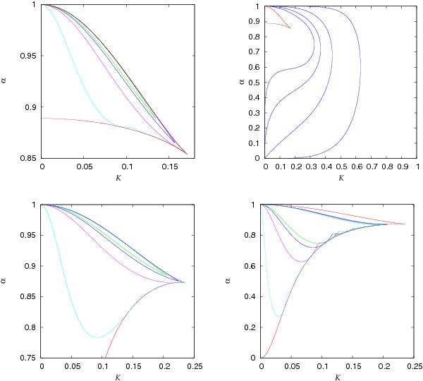
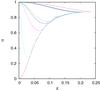
Top left: boundaries of approximating sets for the power spectrum S_r(ω). The function g(x) was evaluated in L points, evenly placed in between g(0) and g(∞). The nested curves correspond to calculated for L equal to 4, 5, 9, and 49. Top right: the nested sets calculated from the upper limit of g′(x). We have taken x₊ = g⁽ⁿ⁾(0) and x₋ = g⁽ⁿ⁾(∞) for n from 1 to 4. Bottom left: the same as in the top left panel for sets . Bottom right: the same as in the bottom left panel, this time with a grid of points that samples the area around point 3h(0) more densely but that does not cover the whole interval ⟨ 3h(0),3h(∞) ⟩. The values of L are the same as in the previous examples. The approximating sets cover a broader part of the whole set . However, they omit a small area of high α. This demonstrates that an adaptive grid can perform significantly better than a regular one.