| Issue |
A&A
Volume 554, June 2013
|
|
|---|---|---|
| Article Number | A143 | |
| Number of page(s) | 26 | |
| Section | Interstellar and circumstellar matter | |
| DOI | https://doi.org/10.1051/0004-6361/201117437 | |
| Published online | 18 June 2013 | |
Time-dependent spectral-feature variations of stars displaying the B[e] phenomenon⋆,⋆⋆,⋆⋆⋆
II. MWC 342
1 Institute of Theoretical Physics and Astrophysics, Masaryk University, 61137 Brno, Kotlářská 2, Czech Republic
2 Astronomical Institute, Charles University in Prague, V Holešovičkách 2, 18000 Praha 8, Czech Republic
e-mail: This email address is being protected from spambots. You need JavaScript enabled to view it.
3 Astronomical Institute of the Academy of Science of the Czech Republic, Fričova 298, 25165 Ondřejov, Czech Republic
Received: 7 June 2011
Accepted: 14 March 2013
Abstract
The B[e] phenomenon can be present in stars of different types and at different evolutionary stages. Very extended circumstellar matter prohibits the study of the atmosphere of these stars, since no photospheric lines are usually observed. Standard stellar atmosphere models are thus not applicable when determining stellar parameters. One of a few possibilities for comprehending the nature of these objects is to study their time variations. Unfortunately, almost no set of spectra with an adequate time description is available for these objects. We obtained an extensive set of MWC 342 spectra (102) during the years 2004–2010 in the wavelength interval around the Hα line (6265–6765 Å) to focus on the time variability of the spectral lines in this region. We chose MWC 342 from the known stars showing the B[e] phenomenon since, although this star is very bright, its evolutionary status and the role of binarity in the appearance of the B[e] phenomenon are unknown. The time dependence of radial velocities and equivalent widths of emission lines was measured for the Hα line, He i 6678 Å, [O i] 6300, 6364 Å, Fe ii 6318, 6384, 6344 and 6456 Å, and Si ii 6347, 6371 Å. We detected variability in the spectral lines on both short and long time scales. He i 6678 Å shows day-to-day changes in its line profile. We observed pure absorption, pure emission, the P Cygni profile, and the inverse P Cygni profile in this line. There are time intervals where this line disappeared. The Hα line also shows considerable changes in its line profile, radial velocities, and equivalent widths. A cycle of about 1560 days was detected in its radial velocities. The detailed description of the variations in MWC 342 spectra reveals its important properties. The inner atmosphere is affected by changes of days, while existing long-term waves are propagated into the outer regions. It is highly probable that the continuum radiation in the visual region is also variable. The inverse P Cygni profile was probably observed when the continuum radiation reached its maximum. These properties indicate the complicated nature of this object. We discuss here a possible explanation of the observations by a stellar wind supported by pulsations.
Key words: stars: individual: MWC 342 / stars: emission-line, Be / stars: mass-loss / binaries: spectroscopic / circumstellar matter
Based on data from the Ondřejov 2 - m telescope, Czech Republic.
Figs. 1, 5, 6, 11, 13, 14, 18, 20, 22, 24 and Appendix A are available in electronic form at http://www.aanda.org
Reduced spectra is only available at the CDS via anonymous ftp to cdsarc.u-strasbg.fr (130.79.128.5) or via http://cdsarc.u-strasbg.fr/viz-bin/qcat?J/A+A/554/A143
© ESO, 2013
1. Introduction
The B[e] phenomenon can be found in different types of objects. Some compact planetary nebulae, Herbig stars, supergiants, and symbiotic stars comprise this group. Owing to the extended circumstellar matter, the nature of many of these objects still remains unrevealed. The distinctive signature of these stars in their optical spectra is the presence of the forbidden emission lines of low-ionised metals, mainly [Fe ii] and [O i] (Lamers et al. 1998). These spectra are typical of their very strong emission of Balmer lines. The permitted emission lines of metals are also present. Another distinctive feature of these objects is strong IR excess due to circumstellar dust.
MWC 342 (V1972 Cyg) shows the B[e] phenomenon. It was first noted as an emission-line star by Merrill & Burwell (1933). Allen (1973) detected infrared excess and interpreted it as a dust contribution. The polarimetric measurements of Zickgraf & Schulte-Ladbeck (1989) show that Mie-scattering is present in this object. They deduced that the dust particles must have a size in the range of 0.08 to 0.1 μm and are composed largely of iron. Based on the photometric observations of Bergner et al. (1990), this star has been included into the General Catalogue of Variable Stars (Kazarovets et al. 1993). The emission lines from forbidden transitions in the spectra indicate the presence of very extended circumstellar matter. The interferometric measurements of Monnier et al. (2006) show a ring structure around the star. They determined not only the diameter of this ring, but also the dust fraction in the media. Direct imaging of this object in the narrow band Hα filter was done by Marston & McCollum (2008). They found a faint structure, however they doubt that it is proof of an ejected material.
Even if MWC 342 has been observed many times, its evolutionary status still remains uncertain. Many authors have supposed that MWC 342 is either in the pre- or in the post-main sequence phase. A detailed discussion of this problem can be found in the paper of Miroshnichenko & Corporon (1999, hereafter MC99). They do not favour the idea of a pre-main sequence star, since MWC 342 does not show any strong far-IR excess. This opinion is also supported by the fact that MWC 342 is not located in a star-forming region. Even if this star is close to the OB9 association (Garmany & Stencel 1992), it is probably not a member, owing to the different polarisation (Zickgraf & Schulte-Ladbeck 1989). The interferometric measurements of Vinković & Jurkić (2007) show that the visibility function of MWC 342 differs from young stellar objects (YSO). On the other hand, Odenwald et al. (1993) classified this star into the YSO group based on CO maser observations. It is probably not a post-AGB object either (MC99), since these objects usually only have far-IR excess and also weaker emission. The hypothesis of a carbon star was excluded by Omont et al. (1993). Due to the lack of emission lines of atoms in high-ionisation stages, the star cannot be a symbiotic star (MC99). The spectrum of this star shows similarities with CI Cam, where a compact object is expected (Frontera et al. 1998). This led MC99 to suggest that MWC 342 is most likely a Be/X-ray system. However, the presence of dust means that this star must have a higher mass-loss rate than classical Be/X-ray systems. Its orbital period must also be longer according to the findings of the dependence between the period and the Hα emission in Be/X-ray systems (Reig et al. 1997).
The first to mention MWC 342 as a binary star were Arkhipova & Ipatov (1982). They estimated the spectral type of the secondary component from the spectrophotometry. They subtracted a B8 star spectrum (Allen & Swings 1972) from the observed spectral energy distribution and a nebular contribution. The resulting fit showed the spectrum of a M0III type star. However, no lines of this spectral type have been found. Later studies by Corporon & Lagrange (1999) also showed no radial velocity variations, but their data set only consisted of a few spectra from 1994.
The binarity, or any other nature of MWC 342, can be determined from its time variability. Especially in this case, the time description becomes very important. Owing to the extended circumstellar matter and lack of photospheric lines in the spectra, the application of commonly used stellar atmosphere codes is impossible. As a result, the time-variability description offers one of the few possibilities for studying these objects. Unfortunately, current studies are only based on a few spectra. A better situation can be found in the photometric observations, but here the variability description is also not satisfactory.
Present photometric studies show irregular variability. A short period from 14 to 16 days has been found in every observing run. Beyond this, a longer period from 40 to 120 days was detected. However, there are some observations where this longer period was not found. The shortest period of 14 days was identified by Shevchenko et al. (1993). Later, Mel’nikov (1997) analysed the data from 1986 to 1994. The amplitude of variations was about a half magnitude using a V filter and then increased towards the longer wavelength. The periods they found changed from year to year. Chkhikvadze et al. (2002) analysed a series of ubvy observations from August and September 1989 and October 1993. They prove that the variability of this star can only be explained when both the gaseous envelope and the circumstellar dust change their properties.
This paper presents seven years of observations of MWC 342, while the spectra of this object was obtained using a slit spectrograph at the 2 - m telescope at Ondřejov observatory (Czech Republic). The observations and data reduction are described in the first part of this paper. Subsequent sections present the results from the primary spectra analysis – time dependencies of radial velocities, equivalent width, and line profile changes. The discussion summarises the common properties of spectral-line behaviour. Finally, we try to interpret these observations.
2. Observations and data reduction
The spectra used in this study were taken during the period 2004 to 2010 with the Coudé spectrograph (Škoda et al. 2002) at the 2 - m telescope in Ondřejov, Czech Republic, using the SITe CCD (2030 × 800 pixels, 15 μm pixel size) in a camera with 700 mm focus. We chose a spectral interval around the Hα line (Fig. 1) from 6265 to 6765 Å, where the resolving power is R ~ 13 000 (~4 px/Å). The list of observations is summarised in Tables A.1–A.3. Some data were obtained in additional spectral ranges of 4760 − 5005 Å (R ~ 18 600, 4 spectra), 5475 − 5985 Å (R ~ 11 500, one spectrum), 7510 − 8020 Å (R ~ 15 500, 7 spectra), and 8200 − 8710 Å (R ~ 16 500, 5 spectra). We did not include the data from these spectral intervals in this paper because we wish to focus here on a description of the time variability, and such a small sample does not allow it.
The data reduction was performed using IRAF1. After the bias subtraction, flat-field and overscan correction, the dcr program written by Pych (2004) was used for the cosmic ray removal. This allowed us to subtract spectra without using the optimal extraction by IRAF apall task. Since these spectra are, with high precision, parallel to the pixel rows, the background, together with the night sky lines, is eliminated during spectra subtraction by individual pixel columns. This is an important step, since the stellar forbidden emission lines are blended by atmospheric night sky lines. The remaining wavelength calibration, heliocentric correction, and the continuum fitting are also performed using IRAF. The last stage, the spectra normalisation, is also one of the key steps, since the Hα emission peak is from fifty to a hundred times more intense than the continuum. Chebyshev polynomial of the third order is used to fit the intervals, which apparently contain no spectral lines. Each continuum interval is split into sub-intervals of five pixels, where the median value is taken for the continuum evaluation. Possible remaining cosmic ray hits thus do not affect continuum normalisation2.
3. Hα variations
3.1. Line profile
The visual spectral range is dominated by a very strong Hα line, which has always been observed as a double-peaked line with a stronger red part. The first who noticed this structure were Swings & Struve (1943). A few decades later, Kuan & Kuhi (1975) also observed this line profile and suggested that this shape can be a combination of a symmetric emission and absorption, which is shifted into the short wavelengths due to a slowly moving shell. The central absorption of the Hα line was observed by MC99 in the high-resolution ÉLODIE spectra. They also had a set of low-resolution spectra (50 and 100 Å/mm) where line profiles were symmetric. MC99 used a convolution with an instrumental profile to prove that this was only due to the low resolution. They showed that Brosch et al. (1978) also had insufficient resolution, so that the observed Balmer lines were symmetric in their data.
Even if the global shape of the Hα line is stable for many decades, the intensity of the line, the equivalent width, the peak ratio, and also the peak shape are very variable. The red peak shows negligible shape changes in our data set, but the changes of the violet peak are very significant (Fig. 2). Mostly, a simple profile is observed; however, there are epochs when the violet peak had a more complicated structure – double and even triple. This complicated structure was found by MC99 in the ÉLODIE spectra at JD 2 449 594.40.
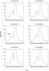 |
Fig. 2 Hα line-profile variability. A set of typical line profiles is plotted. |
The relative flux of the red peak changes from ~ 50 to ~ 100 during our observation period (Fig. 3, left panel). The right hand panel in Fig. 3 shows the maximum (~25) and minimum (~11) relative flux of the violet peak.
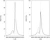 |
Fig. 3 Selected line profiles. Left panel: maximum (JD 2 454 357.47) and minimum (JD 2 455 479.35) intensity of the red peak. Right panel: maximum (JD 2 455 073.46) and minimum (JD 2 454 206.52) intensity of the violet peak. |
3.2. V/R changes
The variations in the peak ratio (violet/red intensity = V/R) have been mentioned previously by MC99. They found V/R values in the ÉLODIE spectra of 0.19 in August 1994 (JD 2 449 594.40), 0.27 in November 1994 (JD 2 449 677.31), and 0.37 in August 1995 (JD 2 449 948.44). Other measurements were reported by Zickgraf (2003). He obtained a V/R ratio (defined by (Fviolet-Fcont)/(Fred-Fcont) in his article) of 0.27 in September 1987 and 0.20 in June 2000. All these previous values are in the range of our measurements (Fig. 4).
To study the variations in the relative flux, an adequate description of the line profile must be achieved. The resolution of the Ondřejov spectrograph gives 4 px/Å in the Hα region. Since our data set is homogeneous, no additional treatment is needed. The intensities were obtained using the MAXIPES program (Mikulášek et al. 2006), where the set of trigonometric functions {1; x; sin(πx); sin(2πx); sin(3πx); ...} is fitted.
The resulting V/R ratio is plotted in Fig. 4. The two maxima of the V/R changes have been captured in our data. The position and the values of these maxima are JD 2 453 614 ± 2, 0.279 ± 0.004, and JD 2 455 084 ± 8, 0.333 ± 0.002. The flattened minimum can also be recognised at JD 2 454 239 ± 9. Its value is 0.159 ± 0.005. We obtained the positions and corresponding values of these extrema by fitting using the MAXIPES code. The dependence of the peak intensities themselves is plotted in Figs. 5 and 6 in the appendix.
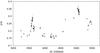 |
Fig. 4 Time dependence of the peak ratio (violet/red) of the Hα emission line from 2004 to 2010. |
3.3. Grey-scale representation
The complex characteristics of the Hα line profile changes is shown in Fig. 7 (upper panel). The plotted value is the ratio of the relative flux and the curve representing the average from all the spectra. The detail for the violet peak is in the lower panel.
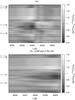 |
Fig. 7 Grey-scale representation of the Hα line. A close-up of the violet part is shown in the bottom panel. The time scale on the y-axis is not conserved. The spectra are sorted by their sequential number from oldest (lowermost) to latest (uppermost). Marks on the left side of the figure point at the special events detected in the iron lines (see Fig. 17). Spectrum denoted by “D” shows an inverse P Cygni profile of the He i 6678 Å line. |
3.4. Equivalent width
The equivalent width (W) of the Hα line changes within the range from − 210 Å to − 370 Å in our data sample (Fig. 8). It corresponds with the previous work of Zickgraf (2003), who found W = − 225 Å in September 1987 and W = − 240 Å in June 2000. Measurements of equivalent width were provided also by MC99. They obtained W = − 246 Å in July 1991 (JD 2 448 456), − 199 Å in August 1994 (JD 2 449 594), − 170 Å in November 1994 (JD 2 449 677) and − 221 Å in August 1995 (JD 2 449 948).
The two previous measurements of MC99 from August and November 1994 are out of the range defined by our data. This implies greater variability on longer time scales; however, probably not much different from the presented one.
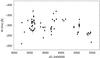 |
Fig. 8 Time dependence of the equivalent width of the Hα line. |
We measured the equivalent width by the numerical integration using a procedure from Ceniga (2004), where the error estimate is adopted from Vollmann & Eversberg (2006). The results are shown in Fig. 8 and listed in Table A.1. A fit with the MAXIPES code finds two minima − 306 ± 5 Å and − 351 ± 12 Å at JD 2 453 675 ± 34 and JD 2 454 444 ± 26, respectively, and a maximum − 266.5 ± 9.4 Å at JD 2 454 068 ± 19 a follow the exact definition of equivalent width in this paper. (The minimum of the equivalent width of emission lines is related to the maximum of their “line strength”.)
3.5. Radial velocity
Radial velocities (RV) of the Hα peaks and central depression were measured previously by MC99. From the ÉLODIE spectra they obtained RV = −136, −82, and −6 km s-1 (violet peak, central depression, and red peak) in August 1994 (JD 2 449 594.40), RV = −149, −88, −11 km s-1 in November 1994 (JD 2 449 677.31) and RV = −133, −83, and −7 km s-1 in August 1995 (JD 2 449 948.44). These values fall within the intervals defined by our data.
We obtained the radial velocities of the Hα peaks and the central depression by fitting the line profile using the MAXIPES code. The central position of the Hα line in the wings is determined by SPectraL Analysis Tool (SPLAT; Draper & Taylor 2009) based on flipping the line profile (so-called flipping or oscilloscopic method).
The mean value of the radial velocity of the violet and red peak is plotted in Fig. 9 (asterisks). Since the radial velocities of the red peak do not change very much (from − 5.3 to + 3.1 km s-1), the time dependence of the radial velocities of the violet peak itself has very similar behaviour. When the violet peak shows a double structure, the corresponding values for both bumps are plotted. An average of the red peak and red bump of the violet peak is denoted by full circles. Empty circles show the values for violet bump for which the linear fit is plotted.
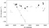 |
Fig. 9 Mean value of radial velocity of Hα peaks (for the symbol explanation see the text). Error bars are in the range of the symbols. |
The radial velocities of the central depression are plotted in Fig. 10. Three extrema are clearly distinguished. Fitting the polynomial function (MAXIPES) to the measured data gives the position and formal error of the two maxima at JD 2 453 758 ± 8 and JD 2 455 201 ± 22 with the values −84.5 ± 0.6 km s-1 and − 83.5 ± 0.2 km s-1, respectively. The minimum is located at the position JD 2 454 244 ± 17. Its value is −95.7 ± 0.4 km s-1.
The time dependence of the radial velocities of the central depression shows a clear trend (Fig. 10). To find possible periods we performed Fourier analysis using Period043 (Lenz & Breger 2005). We searched through all the possible spectra defined by our data. However, no reasonable result was found.
Figure 10 indicates that the data can be fitted by a combination of periodic functions. Considering the fact that a long-term trend is present in the data, we obtained a better fit with a combination of periodic and linear functions  (1)The fityk4 code was used for this purpose, since several methods can be applied (Levenberg-Marquardt, Neldel-Mead simplex, or genetic algorithm). Figure 10 shows the best fit obtained with the parameters a = (0.0028 ± 0.0003) km s-1 day-1, b = (−102 ± 1) km s-1, A = (−4.6 ± 0.3) km s-1, f = (6.4 × 10⁻⁴ ± 1.7 × 10⁻⁵) day-1 (P = (1558 ± 41) days), and φ = (−0.57 ± 0.08) rad. These parameters can describe motion in a binary system, but also can only be connected with the dynamics of the envelope (see the discussion in Sect. 5).
We pay special attention to searching for a period of the order of days (from 0.5 up to 20 days), since a photometric period from 14 to 16 days was detected in previous works. We obtained a fit of our data with a period equal to (1.817 ± 0.007) days. However, this is probably caused by data sampling and only describes the time when the data was observed. To check possible short periods, we removed the global trend (the linear term in Eq. (1)) from our data and again performed a Fourier analysis. A fit of the measured data was obtained with the first two frequencies we found, which is not very convincing since the data sampling can affect the result very much.
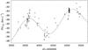 |
Fig. 10 Radial velocities of central depression of the Hα line. The plotted curve is the fit of the periodic function (Eq. (1)). |
The width of the Hα line can be used to test whether the radial velocities of the central depression are connected with binary motion or not. The width at the relative high of 0.1 (0 – continuum; 1 – Hα maximum line intensity) is plotted in Fig. 11, with maxima at JD 2 453 790 ± 20 and JD 2 455 105 ± 24 and a minimum at JD 2 454 400 ± 20. This dependence shows very similar behaviour as the radial velocity of the central depression (Fig. 10). This can be expressed by the Pearson correlation coefficient, whose value is 0.84 in this case.
The variability of the peak separation is shown in Fig. 12. The position of the individual peaks was measured by MAXIPES. If the violet peak shows a complicated structure, the distance between the red peak and bump positions is plotted separately. The position of the Hα line centre in the wings is displayed in Fig. 13. The data scatter and the error intervals suggest that this dependence can be used to search for periodicity. We applied several methods – a discrete Fourier transform (Period04, Lenz & Breger 2005), phase dispersion minimalisation (Stellingwerf 1978; HEC275), and the string-length method (Dworetsky 1983), none of which gave reasonable results.
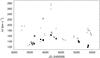 |
Fig. 12 Peak separation ΔV of the Hα line (asterisks). The empty circles denote the difference between the position of the blue bump in the violet peak and red peak. The full circles are values corresponding to the red bump in the violet peak and red peak. |
4. Helium and metal lines
Most of the emission lines are produced by neutral or singly ionised metals. In the range of 6265–6775 Å, where most of our spectra are observed, the major permitted lines come from He i, Fe ii, N i, and Si ii. Moreover, the forbidden lines of [O i] and [N ii] are present. No photospheric lines were found in our spectra, or in the previous work of MC99. Even if they found some absorptions at 6379, 6495, and 6498 Å, they identified them as diffuse interstellar bands.
Helium and metal lines are about an order of magnitude less intensive than the Hα line. They are much more affected by the noise, and therefore not all spectra that could be included for the Hα analysis were used to analyse these lines. The excluded spectra are noticed in Tables A.1–A.3 with measurements.
Due to the low intensity of helium and metal lines, their grey-scale representations (Figs. 15, 17, 19, and 21) do not correspond exactly to the one of the Hα line (Fig. 7). These spectra were limited by the signal-to-noise ratio (S/N) value of 31 so as not to suppress the information in the plots. Spectra affected by residuary cosmics in the current line were also excluded. This restriction did not significantly cut the sample of spectra. At most twenty spectra were excluded.
The equivalent width of metal lines was calculated by the numerical integration. The measurement of the helium line used a script from Polster (2011). The program from Ceniga (2004) was used for the metal lines. The error on these values was in both cases determined using the formula from Vollmann & Eversberg (2006). The radial velocities of the forbidden oxygen lines [O i] 6300 Å and 6364 Å and silicon lines Si ii at 6347 Å and 6371 Å were measured by the profile fitting of the Voigt function in IRAF.
4.1. He I 6678 Å
The He i 6678 Å line is very variable. We observed pure emission and absorption, as well as a P Cygni profile (Fig. 16). Whilst the standard P Cygni profile has already been observed by Andrillat & Jaschek (1999), our data also indicate the presence of an unusual inverse P Cygni profile (JD 2 455 346.49). In some spectra the line almost disappears. The line-profile changes of He i 6678 Å are very fast, exhibiting day-to-day variations. Three series of such spectra are shown in Fig. 14. However, we were not able to find significant changes during one night. The variations in the line profile from all the spectra are shown on the grey-scale representation in Fig. 15. Considering the complicated structure of the He i 6678 Å line (Fig. 16) we do not present the measurements of the equivalent width and radial velocities of this line.
The P Cygni profiles of the He i 6678 Å allow us to estimate the velocity in its line forming region. Its value varies from − 217 km s-1 to − 403 km s-1. Unfortunately, we only have one spectrum in the region 5475–5985 Å, where there is another He i 5876 Å line. On the same night, the Hα region was also obtained. Both He i lines (6678 Å and 6678 Å) had very similar profiles – a pure emission with a small absorption in the blue part.
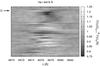 |
Fig. 15 Grey-scale representation of the He i (6678 Å) line. “D” denotes the spectrum showing the inverse P Cygni profile. |
4.2. Iron lines
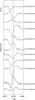 |
Fig. 16 Selected line profiles of the He i 6678 Å. The dashed line represents the laboratory wavelength, the dotted one the central wavelength after the correction on the radial velocity of the MWC 342 system. |
The iron lines in the observed region are represented by Fe ii lines 6318, 6384, 6443, and 6456 Å. The Fe ii 6318 Å line, though relatively intense, is a problem to identify. Zickgraf (2003) identified this line as Mg i. Our decision to classify it as an Fe ii line is based on its similarity to the grey-scale representations with other Fe ii lines. To verify this, we checked the identification of the other B[e] star in our programme, MWC 623. Based on the radial velocity measurements of this star, there is clear evidence that the line at λ = 6318 Å is Fe ii (Polster 2011).
The iron Fe ii 6456 Å line profiles (Fig. 17) change from the emission, which almost has a Gaussian profile to a double and even triple peak shape. These peaks are always slightly violet-shifted compare to the Gaussian-like profile, which is observed around JD ~ 2 454 240. The Gaussian-like profile appears as a bright spot on the grey-scale representations in Fig. 17. The equivalent width dependence (Fig. 18) shows no significant extreme on this date; nevertheless, the data accuracy is not very good. The other iron lines Fe ii 6318, 6384, and 6443 Å show similar behaviour; however, the split lines do not show such a sharp double-peak structure.
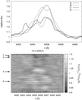 |
Fig. 17 Variations in the Fe ii 6456 Å line. Upper panel: selected line profiles. Lower panel: grey-scale representation from all spectra. A = JD 2 454 240.39, B = JD 2 453 638.39, C = JD 2 455 388.37, D = JD 2 455 346.49. Line profile D corresponds to the appearance of the inverse P Cygni profile in the He i 6678 Å line. |
The equivalent width measurements are plotted in Fig. 18. All iron lines show a smooth trend, where a flattened minimum can be recognised. The position, its value, and the corresponding errors, which were determined by MAXIPES, are summarised in the Table 1.
Minima of the equivalent width of iron lines.
4.3. Oxygen lines
The strongest forbidden lines in our spectra of MWC 342 are the oxygen lines [O i] at 6300 Å and 6364 Å. The variations in the line profiles are shown on the grey-scale representation in Fig. 19. These emission lines had a single peak in our data. However, the [O i] 6300 Å line shows the double-peak structure in the spectra with the better resolution obtained by Zickgraf (2003).
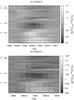 |
Fig. 19 Grey-scale representation of the [O i] lines at λ = 6300 Å (upper panel) and 6364 Å (bottom panel). Notation corresponds with the Fig. 17. The mark “D” points at the spectrum with the inverse P Cygni profile of the He i 6678 Å line. |
The equivalent width variations are presented in Fig. 18. The values are in the range from −1.5 Å to −3.3 Å for [O i] 6300 Å and from −0.55 Å to −1.1 Å for [O i] 6364 Å. The line [O i] 6300 Å is probably more variable than is visible in our data set, since Zickgraf (2003) has obtained a value of its equivalent width of −3.9 Å. The equivalent widths of both lines have very similar time behaviour. We found several extrema in these dependencies using MAXIPES (Table 2).
Extrema of the equivalent width of oxygen lines.
Figure 20 shows the radial velocity measurements of these forbidden oxygen lines. With respect to data accuracy and sampling, we did not search for any periodicity in the radial velocities of [O i] 6300 Å and 6364 Å. The values change in the range from −27 km s-1 to −35 km s-1 for [O i] 6300 Å , and from −25 km s-1 to −36 km s-1 for [O i] 6364 Å.
4.4. Silicon lines
The silicon lines in the chosen interval are represented by Si ii at 6347 Å and 6371 Å. The grey-scale representation of the Si ii 6347 Å line is shown in Fig. 21. The line at λ = 6371 Å shows very similar behaviour. The bright structure that is distinguished well in the grey-scale representation of the Fe ii 6456 Å line (Fig. 17) can also be recognised on the grey-scale representations of silicon lines. The equivalent width measurements are plotted in Fig. 18 in the appendix. The radial velocities of both lines show a huge scatter from ~ –20 to −60 km s-1, but no trend.
5. Discussion
Our observations prove that MWC 342 shows spectral line variations on both short and long time scales.
-
1.
The short time-scale variations are clearly visible on theHe i 6678 Å line. We observed considerable changes in its line profilefrom night to night (Fig. 14). During sevenyears of the observations, the line shape shows pure absorp-tion, pure emission, and also the P Cygni profile. The linedisappeared in some spectra. The inverse P Cygni profilewas also captured. When the inverse P Cygni profile is ob-served, the central line intensity of all lines is almost the low-est one (Fig. 22) and the Fe ii6456 Å lineshows a triple- and double-peak structure(Fig. 17, lines C, D).
-
2.
The line profile variations of the other emission lines are very visible in the grey-scale representations (Figs. 7, 17, 19, and 21). Several events and dependencies can be identified here.
-
i)
Lines of the same element show the same behaviour.
-
ii)
A bright structure (JD ~ 2 454 357) is present in the grey-scale representations of the iron (Fig. 17) and silicon (Fig. 21) lines. This intensity increase is caused by the changing of the double-peak profile to a Gaussian profile (Fig. 17).
-
iii)
The appearance of the Gaussian profile of the iron and silicon lines is connected with the maximum brightening of the Hα red peak (Fig. 7).
-
iv)
This event – where the iron lines show a Gaussian profile – splits the grey-scale representation of all measured lines into two parts. Before this moment, the variation in the line profiles of the iron and oxygen lines are visible; after that, the profile changes of these lines are almost negligible.
-
v)
The maximum depression of oxygen intensity is connected to the maximum depression of silicon intensity (Figs. 19 and 21, JD ~ 2 454 205).
-
vi)
The decrease in intensity of the oxygen (Fig. 19) and silicon (Fig. 21) lines started at the same time as the decrease in intensity of the Hα violet peak (Fig. 7).
-
vii)
The brightening of the Hα violet peak (Fig. 7) occurs at the same time as the maximum brightening of oxygen lines (Fig. 19).
-
i)
-
3.
The radial velocities and equivalent widths of the lines from the same element show the same time behaviour. Several extrema can be found in these dependencies (Figs. 18 and 20; Tables 1 and 2; Sects. 3.4 and 3.5). A summary of all the important events is plotted in Fig. 23. It is possible to see a clear coincidence of the maximum of equivalent width of the forbidden oxygen lines 6300 Å, 6364 Å and the Hα line. The minimum of the radial velocity of the central depression occurs at the same time as the minimum of the intensity ratio of the violet and red peak. This is a natural consequence since the radial velocities of the Hα wings are almost constant; thus the changes of the line profile are caused mainly by the changes of the “central absorption component”.
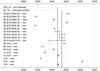
Fig. 23 Timeline of characteristic events in the spectra. The found extrema of the time dependencies of individual spectral quantities are plotted in this figure. V/R denotes the ratio of violet and red peak intensity of the Hα line, rv(CD) denotes the radial velocity of the central depression of the Hα and W extrema of equivalent widths of selected lines. The equivalent width notation follows its definition – negative values denote the emission lines (minima of W in this figure is related to the maxima of “line strength”). The vertical line indicates the time when the iron and silicon line profile become Gaussian (a bright spot on the grey-scale representation in Figs. 17 and 21). Another vertical line shows the time when forbidden oxygen and silicon lines reach their minimum intensity (the darkest spot on the grey-scale representation in Figs. 19 and 21).
The event where the profile of the iron and silicon lines becomes Gaussian is connected with the minimum of the equivalent width of Fe ii 6443 Å and Fe ii 6384 Å. Due to the flattened shape of the equivalent width dependence of iron lines, the error in the extrema determination is large, and it is possible that the iron lines Fe ii 6318 Å and 6456 Å also have their minimum of equivalent width at this time. Close to this event, where the profile of some metal lines becomes Gaussian, the minimum of the radial velocity of the central depression also occurs with the minimum of the violet and red peak intensity ratio and the minimum of the Hα equivalent width.
-
4.
The ratio of equivalent widths of the Fe ii 6318, 6384, 6443 Å, and Si ii 6371 Å with respect to the Hα line are almost constant. The ratios of the equivalent width of Fe ii 6546 Å and Si ii 6347 Å (Fig. 24) to the Hα are slightly variable, especially from the beginning of the observation until JD 2 453 600, where the increase and subsequent decrease in the ratio values are seen. The ratio for both oxygen [O i] lines (Fig. 24) follow the same temporal trend, but the variability is remarkable during the whole observing period.
-
5.
The Hα line is the line whose variability is best described in our observation data set. The changes in the line-profile shape are very strong in the violet part of the Hα line (Fig. 2), where a bump was observed several times. We tried to include these perturbations in all the graphs. We note the radial velocity dependence in Fig. 9. Here the bump in the violet Hα peak is plotted by circles. A straight line can be fitted through the data up to JD 2 454 192. Fitting a straight line would not be possible in the case of a co-rotating structure. This behaviour can more likely indicate an outflowing structure. However, we also detected small moving bumps in the red peak. Unfortunately, due to the low resolution, it is not possible to obtain a reasonable radial velocities of bumps in this part, where the line profile is very steep. The presence of moving bumps in all the line profile more likely indicates a co-rotating structure. Therefore there remains a possibility that the linear fit in the Fig. 9 is a coincidence of the data sampling and insufficient resolution.
-
6.
The inverse P Cygni profile is an important feature in the spectra, since the red-shifted absorption component implies an infall of the material back to the star. In our case, the absorption is more likely situated close to the line rest position (Fig. 16, the upper-most line) than red-shifted. However, a correction to the radial velocity of MWC 342 must be applied. The average of the radial velocities of the oxygen forbidden emission lines (RV = −31.103 ± 0.011 km s-1) can be used for this purpose, since they originate in the outer diluted parts of the media, and their width indicates a not very high velocity gradient. After this correction, the central absorption of the inverse P Cygni profile shifts to the red side (Fig. 16). This allows us to suppose that we observed the infall of the material. The appearance of the inverse P Cygni profile in stars with the B[e] phenomenon is rare, but it has been observed previously. Several spectral lines with this line-profile shape were detected in MWC 158 – O i triplet 7773 Å (Andrillat & Houziaux 1991), He i 5876 Å (Bopp 1993; Pogodin 1997; Borges Fernandes et al. 2009), and Si ii lines 6347 and 6371 Å (Borges Fernandes et al. 2009). The He i 5876 Å line with the inverse P Cygni profile was observed by Israelian & Musaev (1997) in MWC 142. They also mentioned the Mg ii 4481 Å line with this line profile. This line shows very similar behaviour to He i 6678 Å in our observations of MWC 342 – pure absorption, pure emission, P Cygni, and inverse P Cygni profile changing on the scale of several days. The inverse P Cygni profile has always been temporally restricted and appears irregularly. The explanations of such line profile changes have been proposed as i) a pre-main-sequence model of T Tauri stars; ii) a component decoupling in the stellar wind; iii) ionisation of accelerating particles in the stellar wind; iv) clumping in the stellar wind; v) co-rotating interaction regions; vi) rotation of the circumstellar disc (V/R changes); vii) a mass transfer binary; or viii) pulsations.
-
i)
a pre-main-sequence model of T Tauri stars A model of T Tauri stars (e.g. Pudritz 1985) seems to be very promising. Both an internal accretion and an external outflowing wind region are present there. Moreover, Herbig pre-main-sequence stars create a group of stars showing the B[e] phenomenon. However, signatures exist that exclude a pre-main-sequence scenario (see Sect. 1).
-
ii)
a component decoupling in the stellar wind The drift kinetic energy of the individual wind components can be higher than the thermal energy of the wind particles in B and A stars. When this occurs, the interaction between components rapidly decreases, and the components that are not sufficiently accelerated by the radiation slow down. Krtička et al. (2006) prove on the model of σ Ori E (B2Vp) that He does not decouple. He-decoupling is possible only for almost neutral helium.
-
iii)
ionisation of accelerating particles in the stellar wind If the medium is sufficiently heated, the particles responsible for the acceleration can be ionised, and the wind is not accelerated further. The additional heating can be provided by shock waves (Krolik & Raymond 1985). This is perhaps one of the promising processes that can explain the observed properties. The shock waves are created close to the photosphere and mostly affect this region. The fallback of the material will thus not be observed in lines that form in the outer region. However, hydrodynamic calculations are needed to show if the temperature in the shocks is high enough to ionise the accelerating particles.
-
iv)
clumping in the stellar wind Israelian & Musaev (1997) suggested that the inverse P Cygni profile observed in MWC 142 can be caused by clouds with different properties present in the wind. The hydrodynamic simulations (Owocki 2008) show that although clumps can have a negative velocity relative to each other, they still accelerate relative to the deep atmosphere. Therefore “real” inverse P Cygni profiles can hardly be produced.
-
v)
co-rotating interaction regions (CIRs) Pogodin (1997) observed the same behaviour in MWC 158. He suggested the explanation of rotating inhomogeneities. However, to explain a red-shifted absorption, the infall of the media is necessary. Hydrodynamic calculations by e.g. Cranmer & Owocki (1996) show outflowing spiral arms that create a small moving absorption (discrete absorption component), but do not change the line profile significantly.
-
vi)
rotation of the circumstellar disc (V/R changes) The line profile shape can be affected by similar processes that are responsible for V/R changes in classical Be stars. A (elliptical) rotating outflowing disc can explain the observed properties (Struve 1931; McLaughlin 1961a,b). However, also in this case, matter infall is needed to create a “true” inverse P Cygni profile.
-
vii)
mass transfer binary The Be star β Lyr shows the similar behaviour of the line-profile variations of He i 6678 Å as in MWC 342. As β Lyr is a very bright star, it has been observed frequently. Based on photometric, spectroscopic, and interferometric observations, Harmanec et al. (1996) proposed a new model: binary with mass transfer, where the stream creates an accretion disc with a hot spot and jets. The combination of all these parts is responsible for the complicated line profiles.
-
viii)
pulsations Many hot stars are radial or non-radial pulsators. Cranmer (2009) discuss the connection between pulsations and disc formation in Be stars in detail from both the theoretical viewpoint and from observational evidence. He shows that the resonance of non-radial pulsations can lead to the formation of waves that propagate outwards and create a shock wave. This process can support the material in the Keplerian disc. Unfortunately, the parameters of MWC 342 are not determined well enough to verify that the star is placed in an instability strip. Its effective temperature (Teff = 26 000 K, MC99) indicates that MWC 342 can occupy an instability strip of β Cephei stars, slowly pulsating B (SPB) stars (pre- and post-TAMS), and slowly pulsating B-supergiants. The changes in the line profiles of He i 6678 Å on the scale of days and probable evolution stage (Sect. 1) point to the group of post-TAMS SPB stars.
-
i)
-
7.
The binary nature of MWC 342 is assumed by many authors. In the detailed review of MC99, they concluded that it is probably a binary with a period longer than forty years. It is very difficult to verify this hypothesis since i) there is no such long data series of observations; and ii) no photospheric absorption lines are observed, therefore the radial velocity changes can be connected to variable envelope properties. We analysed the radial velocities of the central depression of the Hα line (Fig. 10). We expected a very long period (fitted by a straight line) combined with a period of several years (Eq. (1)). The found “period” is (1558 ± 41) days. However, distinguishing between a binary origin and a physical phenomenon in the envelope requires at least simple modelling. In this system, not only may two (three) stellar components play a role, but also the very extended and variable gas envelope, as well as dust, whose contribution is also variable (Chkhikvadze et al. 2002). As one of the test criteria of such a model, the correlation between the radial velocity of the central depression and the width of the Hα wings can be used. Both dependencies show very similar time behaviour, expressed by a Pearson correlation coefficient of 0.84. Moreover, the interval between minima of the equivalent width of the Hα line is (769 ± 43) days, which is roughly half of the “period” found from the fitting of the central depression dependence.
-
8.
A rotating disc itself is not able to explain observed properties (Sect. 5, 2d paragraph). The multiple peaks of the iron line (Fig. 17) are violet-shifted before and also after the appearance of the narrow Gaussian profile. This reflects the negative radial velocity motion in both situations, which excludes the possible explanation using spiral arms.
-
Stellar wind supported by pulsations can be a prospective explanation. It links together the observed properties described in this paper:
-
i)
The He i 6678 Å line changes of the order of days (Fig. 14). This line was observed in absorption, emission, with both the P Cygni and the inverse P Cygni profile (Fig. 16).
-
ii)
When the inverse P Cygni profile appears, a significant decrease in line intensities is observed in all lines in the chosen interval (6265–6765 Å). The decrease in line intensities in all lines simultaneously can be explained only by an increase in continuum radiation. The changes in the “stellar radius”, and connected temperature changes, are usually responsible for this effect.
-
iii)
The Fe ii 6456 Å line profile has multiple emission peaks, but also shows a pure Gaussian profile. The multiple emission peaks are always observed as slightly violet-shifted compared to the Gaussian profile (similar as in Fig. 17). This is an indication that the Fe ii line-forming region expanded during some observing intervals. The multiple emission peaks can appear only in the case where the multiple expanding layers with different velocities are present in the atmosphere.
-
iv)
The forbidden transitions allow forbidden lines to only be formed in the diluted outer parts. Since these lines are very narrow, the velocity gradient in their line-forming region must be small. Since the absorption probability in the forbidden lines is very low, the transparency in these lines is very high. Their line-forming region is a significant part of the envelope if not almost all the envelope. The lines are affected by the velocity ± v∞. This implies that not only the gradient of the velocity, but also its absolute value must be low. This in turn indicates that the expanding layers significantly lose their kinetic energy. As the velocity of the moving layers decreases, the line profiles become narrow and symmetric. A Gaussian-like profile appears for every line at the same time that it is observed. When no other layers or shock waves appear in the atmosphere, the line profiles do not change significantly, and the grey-scale representation shows no differences, as we can see in Figs. 7, 17, 19, and 21. One of the possible mechanisms for the slowing down of the material may be a component decoupling of the wind. The calculations of Porter & Drew (1995) show that the wind decoupling of a B2V star occurs before the wind reaches its escape velocity. The consequences of this effect are discussed further in Porter & Skouza (1999).
-
v)
The radial velocity of the bump in the violet part of the Hα line shows a linear time dependence in the first part of our observing epoch. This is evidence of expanding matter. However, this last point is less relevant. Our observations could not unambiguously exclude that the moving bumps are a consequence of the co-rotating region. This linear fit can only be an effect of the data sampling. On the other hand, the co-rotating region itself is not able to explain previous points i)–iv).
-
i)
The hydrodynamic calculations, together with radiative transfer, are needed to prove what is a guess in this particullar case. The previous theoretical works, which are dedicated to the study of the influence of the stellar pulsations on the radiatively driven wind, indicate that this can be a possible scenario. Cranmer & Owocki (1996) assumed that the resonance of the multiple modes of non-radial pulsations can form a bright or dark spot at the stellar surface. They showed that these brightness changes lead to the large-scale structures in the wind. They especially demonstrated that the discontinuity in the velocity gradient appears and forms a “kink” and a flat velocity plateau. These velocity gradient changes affect the line profile much more than the density difference of the moving shells. The propagation of kinks through stellar wind is discussed by Feldmeier et al. (2008).
There is also a minor observational support. The variable star BW Vul belongs to the group of β Cephei. It is a radial pulsator, whose amplitude is the largest known in the Galaxy. The shock waves have been proved to propagate through its atmosphere (Smith & Jeffery 2003). MWC 342 can fall into the range of β Cephei variable according to the errorbars of derived stellar parameters. Moreover, the radial velocity amplitude changes from cycle to cycle. Unfortunately, due to the lack of atmospheric lines and unsufficient temporal description of photometric observations, there was not possible to confirm this guess.
6. Conclusions
MWC 342 is a very interesting object that shows the B[e] phenomenon. Since the central star is hidden in the circumstellar matter, it is questionable to use standard synthetic spectra for its analysis. Therefore, we focussed on searching for time variability of the spectral lines, which can be very useful for determining the nature of this object. The spectral interval 6265–6775 Å was monitored for seven years from 2004 to 2010.
Our observations proved that this object is variable on both short- and long-time scales. Some events in the spectral-line features appeared after a “period” about 1560 days. However, longer observation series or theoretical modelling is needed to determine whether this “period” is connected with the binary motion or changes in stellar envelope properties.
We found proof of outflowing material. The P Cygni profile was observed for the He i 6678 Å line. The Fe ii 6456 Å line profiles and the radial velocities of the bump in the violet peak of the Hα line also support the idea of material outflow. Moreover, peaks of the multiple profile of the Fe ii 6456 Å line are shifted to the violet compared to the central wavelength defined by the Gaussian profile (Fig. 17). The signature of the material infall was also detected – an inverse P Cygni profile. The inverse P Cygni profile appeared at the same time when the line intensities of all the lines were almost the lowest. This indicates changes in stellar continuum radiation, which is usually caused by stellar radius variations and associated temperature changes. The profile of iron lines is very variable. It changes from multiple emission peaks to an almost Gaussian line profile. We suggest that all this behaviour may be explained by the stellar wind supported by pulsations, where the multiple expanding layers form in the outer parts. However, further detailed calculations are necessary to confirm this guess.
Although our observations did not reveal the nature of MWC 342 in detail, they set up important goals for future investigation. A description of the He i 6678 Å line-profile variations, especially in view of the appearance of the P Cygni and inverse P Cygni profiles, can be very important for investigating the processes leading to the origin of large mass loss in B[e] stars (wind-pulsation connection). The stellar pulsations can reveal themselves by the connection between the He i 6678 Å line profile and the short photometric period of about fifteen days. Determining the origin of the variations – the binary nature, the stellar wind, or the stellar wind supported by pulsations – can made by theoretical modelling of the observed quantities. The data presented in this paper are essential especially for this last point. The modelling of such a complicated system, where the expanded atmosphere together with dust production play a role, is affected by a large set of free parameters. The time variability description of the spectra properties gives a sharp restriction on the theoretical model.
Online material
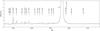 |
Fig. 1 Line identification of MWC 342. Two diffuse interstellar bands (DIB) identified by MC99 was also seen. |
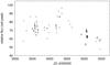 |
Fig. 5 Relative flux of the Hα red peak. |
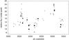 |
Fig. 6 Relative flux of the Hα violet peak (asterisks). The circles denote the value for the bump, if it is present. |
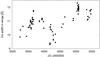 |
Fig. 11 Hα width at the relative height 0.1 (0 – continuum; 1 – Hα line intensity). The error bars are in the size of the symbols. |
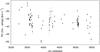 |
Fig. 13 Radial velocity of the Hα line centre in the wings. |
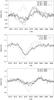 |
Fig. 14 Variations of He i 6678 Å line profile during three nights in July 2005, April 2007, and two nights in September 2009. |
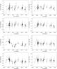 |
Fig. 18 Equivalent width of metal lines. |
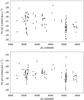 |
Fig. 20 Radial velocity of [O i]. The line at λ = 6300 Å (upper panel) and 6364 Å (bottom panel). |
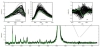 |
Fig. 22 All the spectra from the Hα region. The spectrum showing the inverse P Cygni profile of the He i 6678 Å is displayed by the green line. The details of the Hα wings and He i 6678 Å are shown on the top of the figure. |
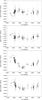 |
Fig. 24 Ratio of the equivalent width of metal lines and equivalent width of Hα. |
Appendix A: List of observations and table of measurements.
List of observations and measured values of the Hα line.
List of observations and measured values of equivalent width of iron lines.
List of observations and measured values of oxygen and silicon lines.
IRAF is distributed by the National Optical Astronomy Observatories, operated by the Association of Universities for Research in Astronomy, Inc., under contract to the National Science Foundation of the United States.
Data are available at the CDS.
Acknowledgments
We would like to thank P. Koubský, Z. Mikulášek and P. Harmanec for their notes and advice. Our thanks go also to A. Kawka, M. Dovčiak and P. Hadrava for their help in obtaining spectra and M. Ceniga for providing a script for the data analysis. This research is partly financed by the Research Program MSM0021620860 (MŠMT ČR) and grant 205/09/P476 (GA ČR). The Astronomical Institute in Ondřejov is supported by the project AV0Z10030501.
References
- Allen, D. A. 1973, MNRAS, 161, 145 [NASA ADS] [Google Scholar]
- Allen, D. A., & Swings, J. P. 1972, Ap, 10, L83 [Google Scholar]
- Andrillat, Y., & Houziaux, L. 1991, IAUC, 5164, 3 [NASA ADS] [Google Scholar]
- Andrillat, Y., & Jaschek, C. 1999, A&AS, 136, 59 [NASA ADS] [CrossRef] [EDP Sciences] [Google Scholar]
- Arkhipova, V. P., & Ipatov, A. P. 1982, Sov. Astron. Lett., 8, 298 [Google Scholar]
- Bergner, Yu. K., Miroshnichenko, A. S., Sudnik, I. S., et al. 1990, Afz, 32, 203 [NASA ADS] [Google Scholar]
- Bopp, B. W. 1993, IBVS, 3834, 1 [NASA ADS] [Google Scholar]
- Borges Fernandes, M., Kraus, M., Chesneau, O., et al. 2009, A&A, 508, 309 [NASA ADS] [CrossRef] [EDP Sciences] [Google Scholar]
- Brosch, N., Leibowitz, E. M., & Spector, N. 1978, A&A, 65, 259 [NASA ADS] [Google Scholar]
- Ceniga, M. 2004, Master Thesis, Masaryk University, Brno, Czech Republic [Google Scholar]
- Chkhikvadze, J. N., Kakhiani, V. O., & Djaniashvili, E. B. 2002, Astrophys., 45, 8 [NASA ADS] [CrossRef] [Google Scholar]
- Corporon, P., & Lagrange, A. M. 1999, A&AS, 136, 429 [NASA ADS] [CrossRef] [EDP Sciences] [Google Scholar]
- Cranmer, S. R. 2009, ApJ, 701, 396 [NASA ADS] [CrossRef] [Google Scholar]
- Cranmer, S. R., & Owocki, S. P. 1996, ApJ, 462, 469 [NASA ADS] [CrossRef] [Google Scholar]
- Draper, P. W., & Taylor, M. 2009, Starlink User Note 243.39, CCLRC/ Rutherford Appleton Laboratory [Google Scholar]
- Dworetsky, M. M. 1983, MNRAS, 203, 917 [NASA ADS] [Google Scholar]
- Feldmeier, A., Rätzel, D., & Owocki, S. P. 2008, ApJ, 679, 704 [NASA ADS] [CrossRef] [Google Scholar]
- Frontera, F., Orlandini, M., Amati, L., et al. 1998, A&A, 339, L69 [NASA ADS] [Google Scholar]
- Garmany, C. D., & Stencel, R. E. 1992, A&AS, 94, 211 [NASA ADS] [Google Scholar]
- Harmanec, P., Morand, F., & Bonneau, D., 1996, A&A, 312, 879 [NASA ADS] [Google Scholar]
- Israelian, G., & Musaev, F. 1997, A&A, 328, 339 [NASA ADS] [Google Scholar]
- Kazarovets, E. V., Samus, N. N., & Goranskij, V. P. 1993, IBVS, No. 3840 [Google Scholar]
- Kuan, P., & Kuhi, L. V. 1975, ApJ, 199, 148 [NASA ADS] [CrossRef] [Google Scholar]
- Kučerová, B 2011, Ph.D. Thesis, Masaryk University, Brno, Czech Republic [Google Scholar]
- Krolik, J. H., & Raymond, J. C. 1985, ApJ, 298, 660 [NASA ADS] [CrossRef] [Google Scholar]
- Krtička, J., Kubát, J., & Groote, D. 2006, A&A, 460, 145 [Google Scholar]
- Lamers, H. J. G. L. M., Zickgraf, F. J., de Winter, D., et al. 1998, A&A, 340, 117 [NASA ADS] [Google Scholar]
- Lenz, P., & Breger, M. 2005, Commun. Asteros., 146, 53 [Google Scholar]
- Marston, A. P., & McCollum, B. 2008, A&A, 477, 193 [NASA ADS] [CrossRef] [EDP Sciences] [Google Scholar]
- McLaughlin, D. B. 1961a, J. Roy. Astron. Soc. Canada, 55, 13 [NASA ADS] [Google Scholar]
- McLaughlin, D. B. 1961b, J. Roy. Astron. Soc. Canada, 55, 73 [Google Scholar]
- Mel’nikov, S. Yu. 1997, Astron. Lett., 23, 799 [NASA ADS] [Google Scholar]
- Merrill, R. W., & Burwell, C. G. 1933, AJ, 78, 87 [Google Scholar]
- Mikulášek, Z., Wolf, M., Zejda, M., & Pecharová, P. 2006, Ap&SS, 304, 363 [NASA ADS] [CrossRef] [Google Scholar]
- Miroshnichenko, A. S., & Corporon, P. 1999, A&A, 349, 126 [NASA ADS] [Google Scholar]
- Monnier, J. D., Berger, J.-P., Millan-Gabet, R., et al. 2006, ApJ, 647, 444 [NASA ADS] [CrossRef] [Google Scholar]
- Odenwald, S. F., & Schwartz, P. R. 1993, ApJ, 405, 706 [NASA ADS] [CrossRef] [Google Scholar]
- Omont, A., Loup, C., Forveille, T., et al. 1993, A&A, 267, 515 [NASA ADS] [Google Scholar]
- Owocki, S. P. 2008, in Clumping in Hot-Star Winds, eds. W.-R. Hamann, A. Feldmeier, & L. M. Oskinova, 121 [Google Scholar]
- Pogodin, M. A. 1997, A&A, 317, 185 [NASA ADS] [Google Scholar]
- Polster, J. 2011, Ph.D. Thesis, Masaryk University, Brno, Czech Republic [Google Scholar]
- Porter, J. M., & Drew, J. E. 1995, A&A, 296, 761 [NASA ADS] [Google Scholar]
- Porter, J. M., & Skouza, B. A. 1999, A&A, 344, 205 [NASA ADS] [Google Scholar]
- Puls, J., Sundqvist, J., O., & Rivero González, J. G. 2011, IAUS, 272, 554 [NASA ADS] [Google Scholar]
- Pudritz, R. E. 1985, ApJ, 293, 216 [NASA ADS] [CrossRef] [Google Scholar]
- Pych, W. 2004, PASP, 116, 148 [NASA ADS] [CrossRef] [Google Scholar]
- Reig, P., Fabregat, J., & Coe, M. J. 1997, A&A, 322, 193 [NASA ADS] [Google Scholar]
- Shevchenko, V. S., Grankin, K. N., Ibragimov, M. A., Mel’Nikov, S. Yu., & Yakubov, S. D. 1993, Ap&SS, 202, 121 [NASA ADS] [CrossRef] [Google Scholar]
- Škoda, P., Šlechta, M., & Honsa, J. 2002, PAICz, 90 [Google Scholar]
- Smith, M. A., & Jeffery, C. S. 2003, MNRAS, 341, 1141 [NASA ADS] [CrossRef] [Google Scholar]
- Stellingwerf, R. F. 1978, ApJ, 224, 953 [NASA ADS] [CrossRef] [Google Scholar]
- Struve, O. 1931, ApJ, 73, 94 [NASA ADS] [CrossRef] [Google Scholar]
- Swings, T. P., & Struve, O. 1943, AJ, 97, 194 [NASA ADS] [CrossRef] [Google Scholar]
- Vinković, D., & Jurkić, T. 2007, ApJ, 658, 462 [NASA ADS] [CrossRef] [Google Scholar]
- Vollmann, K., & Eversberg, T. 2006, Astron. Nachr., 9, 865 [Google Scholar]
- Zickgraf, F. J. 2003, A&A, 408, 257 [NASA ADS] [CrossRef] [EDP Sciences] [Google Scholar]
- Zickgraf, F.-J., & Schulte-Ladbeck, R. E. 1989, A&A, 214, 274 [NASA ADS] [Google Scholar]
- Zickgraf, F. J., Wolf, B., Stahl, O., Leitherer, C., & Klare, G. 1985, A&A, 143, 421 [NASA ADS] [Google Scholar]
All Tables
All Figures
|
Fig. 2 Hα line-profile variability. A set of typical line profiles is plotted. |
| In the text | |
|
Fig. 3 Selected line profiles. Left panel: maximum (JD 2 454 357.47) and minimum (JD 2 455 479.35) intensity of the red peak. Right panel: maximum (JD 2 455 073.46) and minimum (JD 2 454 206.52) intensity of the violet peak. |
| In the text | |
|
Fig. 4 Time dependence of the peak ratio (violet/red) of the Hα emission line from 2004 to 2010. |
| In the text | |
|
Fig. 7 Grey-scale representation of the Hα line. A close-up of the violet part is shown in the bottom panel. The time scale on the y-axis is not conserved. The spectra are sorted by their sequential number from oldest (lowermost) to latest (uppermost). Marks on the left side of the figure point at the special events detected in the iron lines (see Fig. 17). Spectrum denoted by “D” shows an inverse P Cygni profile of the He i 6678 Å line. |
| In the text | |
|
Fig. 8 Time dependence of the equivalent width of the Hα line. |
| In the text | |
|
Fig. 9 Mean value of radial velocity of Hα peaks (for the symbol explanation see the text). Error bars are in the range of the symbols. |
| In the text | |
|
Fig. 10 Radial velocities of central depression of the Hα line. The plotted curve is the fit of the periodic function (Eq. (1)). |
| In the text | |
|
Fig. 12 Peak separation ΔV of the Hα line (asterisks). The empty circles denote the difference between the position of the blue bump in the violet peak and red peak. The full circles are values corresponding to the red bump in the violet peak and red peak. |
| In the text | |
|
Fig. 15 Grey-scale representation of the He i (6678 Å) line. “D” denotes the spectrum showing the inverse P Cygni profile. |
| In the text | |
|
Fig. 16 Selected line profiles of the He i 6678 Å. The dashed line represents the laboratory wavelength, the dotted one the central wavelength after the correction on the radial velocity of the MWC 342 system. |
| In the text | |
|
Fig. 17 Variations in the Fe ii 6456 Å line. Upper panel: selected line profiles. Lower panel: grey-scale representation from all spectra. A = JD 2 454 240.39, B = JD 2 453 638.39, C = JD 2 455 388.37, D = JD 2 455 346.49. Line profile D corresponds to the appearance of the inverse P Cygni profile in the He i 6678 Å line. |
| In the text | |
|
Fig. 19 Grey-scale representation of the [O i] lines at λ = 6300 Å (upper panel) and 6364 Å (bottom panel). Notation corresponds with the Fig. 17. The mark “D” points at the spectrum with the inverse P Cygni profile of the He i 6678 Å line. |
| In the text | |
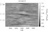 |
Fig. 21 Grey-scale representation of the Si ii 6347 Å line. Notation corresponds with the Fig. 17. |
| In the text | |
|
Fig. 23 Timeline of characteristic events in the spectra. The found extrema of the time dependencies of individual spectral quantities are plotted in this figure. V/R denotes the ratio of violet and red peak intensity of the Hα line, rv(CD) denotes the radial velocity of the central depression of the Hα and W extrema of equivalent widths of selected lines. The equivalent width notation follows its definition – negative values denote the emission lines (minima of W in this figure is related to the maxima of “line strength”). The vertical line indicates the time when the iron and silicon line profile become Gaussian (a bright spot on the grey-scale representation in Figs. 17 and 21). Another vertical line shows the time when forbidden oxygen and silicon lines reach their minimum intensity (the darkest spot on the grey-scale representation in Figs. 19 and 21). |
| In the text | |
|
Fig. 1 Line identification of MWC 342. Two diffuse interstellar bands (DIB) identified by MC99 was also seen. |
| In the text | |
|
Fig. 5 Relative flux of the Hα red peak. |
| In the text | |
|
Fig. 6 Relative flux of the Hα violet peak (asterisks). The circles denote the value for the bump, if it is present. |
| In the text | |
|
Fig. 11 Hα width at the relative height 0.1 (0 – continuum; 1 – Hα line intensity). The error bars are in the size of the symbols. |
| In the text | |
|
Fig. 13 Radial velocity of the Hα line centre in the wings. |
| In the text | |
|
Fig. 14 Variations of He i 6678 Å line profile during three nights in July 2005, April 2007, and two nights in September 2009. |
| In the text | |
|
Fig. 18 Equivalent width of metal lines. |
| In the text | |
|
Fig. 20 Radial velocity of [O i]. The line at λ = 6300 Å (upper panel) and 6364 Å (bottom panel). |
| In the text | |
|
Fig. 22 All the spectra from the Hα region. The spectrum showing the inverse P Cygni profile of the He i 6678 Å is displayed by the green line. The details of the Hα wings and He i 6678 Å are shown on the top of the figure. |
| In the text | |
|
Fig. 24 Ratio of the equivalent width of metal lines and equivalent width of Hα. |
| In the text | |
Current usage metrics show cumulative count of Article Views (full-text article views including HTML views, PDF and ePub downloads, according to the available data) and Abstracts Views on Vision4Press platform.
Data correspond to usage on the plateform after 2015. The current usage metrics is available 48-96 hours after online publication and is updated daily on week days.
Initial download of the metrics may take a while.