| Issue |
A&A
Volume 552, April 2013
|
|
|---|---|---|
| Article Number | A1 | |
| Number of page(s) | 9 | |
| Section | Extragalactic astronomy | |
| DOI | https://doi.org/10.1051/0004-6361/201321047 | |
| Published online | 13 March 2013 | |
Size and disk-like shape of the broad-line region of ESO 399-IG20
1 Astronomisches Institut, Ruhr–Universität Bochum, Universitätsstraße 150, 44801 Bochum, Germany
e-mail: This email address is being protected from spambots. You need JavaScript enabled to view it.
2 Instituto de Astronomia, Universidad Católica del Norte, Avenida Angamos 0610, Casilla 1280 Antofagasta, Chile
3 Department of Physics, University of Oxford, Keble Road, Oxford OX1 3RH, UK
Received: 6 January 2013
Accepted: 5 February 2013
Abstract
We present photometric reverberation mapping of the narrow-line Seyfert 1 galaxy ESO 399-IG20 performed with the robotic 15 cm telescope VYSOS-6 at the Cerro Armazones Observatory. Through the combination of broad- and narrow-band filters we determine the size of the broad-line emitting region (BLR) by measuring the time delay between the variability of the continuum and the Hα emission line. We use the flux variation gradient method to separate the host galaxy contribution from that of the active galactic nucleus (AGN), and to calculate the 5100 Å luminosity LAGN of the AGN. Both measurements permit us to derive the position of ESO 399-IG20 in the BLR size – AGN luminosity RBLR ∝ LAGN0.5 diagram. We infer the basic geometry of the BLR through modeling of the light curves. The pronounced sharp variability patterns in both the continuum and the emission line light curves allow us to reject a spherical BLR geometry. The light curves are best fitted by a disk-like BLR seen nearly face-on with an inclination angle of 6° ± 3° and with an extension from 16 to 20 light days.
Key words: galaxies: active / galaxies: Seyfert / galaxies: distances and redshifts / galaxies: individual: ESO 399-IG20 / quasars: emission lines
© ESO, 2013
1. Introduction
The physical properties of the broad line region (BLR) in active galactic nuclei (AGN) have been extensively studied during the past three decades. Consensus has been reached that the luminosity variations of the continuum emitting region of the hot accretion disk produce variations of the broad emission lines with a delay due to the light travel time across the BLR. To date, the only method independent on spatial resolution is reverberation mapping (Blandford & McKee 1982; Peterson 1993), in which one measures the time delay or “echo” between the continuum variability and the variability observed in the broad emission lines. This method has been used successfully for determining the BLR size, kinematics and black hole mass (MBH) of several Type-1 AGNs. RM provides basic MBH estimates through the virial product  , where G is the gravitational constant, RBLR = c·τ is the BLR size, σV is the emission-line velocity dispersion of the BLR gas and the factor f depends on the – so far unknown – geometry and kinematics of the BLR (Peterson et al. 2004 and references therein). Furthermore, as a widely used extrapolation of locally obtained RM results to higher redshift data, MBH has be estimated using the BLR Size-Luminosity
  relationship (Koratkar & Gaskell 1991; Kaspi et al. 1996, 2000; Wandel et al. 1999; McGill et al. 2008; Vestergaard et al. 2011). However, a reliable MBH estimation from the luminosity requires a considerable reduction of the R − L dispersion present.
As the size of the BLR ranges from a few to several hundred light days, it is necessary to perform observational monitoring campaigns ranging from months to years in order to sufficiently sample the time domain of the echo. Most observational RM campaigns have used spectroscopic monitoring of the sources, which however requires large amounts of telescope time.
Recently, Haas et al. (2011) proposed photometric reverberation mapping (PRM) as an efficient method to determine the BLR size through the use of broad band filters to trace the AGN continuum variations and narrow-band filters to catch the BLR emission line response. Because the narrow-band collects both the emission line flux and the underlying continuum, the challenge is to extract the pure emission line light curve. In the dedicated case study of 3C 120, Pozo Nuñez et al. (2012) demonstrated that PRM reaches an accuracy similar to spectroscopic RM (Grier et al. 2012).
Another efficient approach to determine the BLR size has been proposed by Chelouche & Daniel (2012), through the analysis of the difference between the cross-correlation (CCF) and the auto-correlation (ACF) functions for suitably chosen broad band filters, one filter covering a bright emission line and one covering only the continuum. While this method does not place a strict requirement on the object’s redshift such that the emission line falls into the narrow-band filter (as in the case proposed by Haas et al. 2011), the use of broad band filters only (as proposed by Chelouche & Daniel 2012) limits the application of PRM to cases with a sufficiently strong emission line contribution in the respective filter used. Despite of this handicap, this method has been successfully applied to determine the BLR size for one low-luminosity AGN NGC 4395 (Edri et al. 2012) and one high-z luminous MACHO quasar (Chelouche et al. 2012) consistent with previous spectroscopic RM results.
A fundamental issue in both these methods is to separate the host-galaxy contribution from the total luminosity to calculate the AGN luminosity. An incorrect determination of the nuclear AGN luminosity (due to the contamination of the host component) causes an overestimation of the linear regression slope α. This has been demonstrated by Bentz et al. (2009), who presented the most recent compilation of host-subtracted AGN luminosities for several reverberation-mapped Seyfert 1 galaxies obtained through host-galaxy modeling of high-resolution Hubble Space Telescope (HST) images. Compared to the previous slope of α = 0.7 they determined an improved slope of  close to α = 0.5 expected from photo-ionization models of the BLR (Davidson & Netzer 1979). A different approach to estimate the host galaxy contribution is the flux variation gradient method (FVG, Choloniewski 1981; Winkler 1997). An advantage is that it does not require high spatial resolution imaging and can be applied directly to the monitoring data. Recently, FVG has been tested on PRM data (Haas et al. 2011; Pozo Nuñez et al. 2012). These tests show that by using a well defined range for the host galaxy slope (Sakata et al. 2010) it is possible to separate the AGN contribution at the time of the monitoring campaigns.
ESO 399-IG20 has been classified as a Narrow-Line Seyfert 1 (NLS1) galaxy (Véron-Cetty & Véron 2010). It has often been speculated that the lack of broad emission lines of – at least – part of the NLS1 population can be explained by face-on disk-like BLR geometries. Single-epoch spectroscopic investigations by Dietrich et al. (2005) show high-ionized gas orbiting at high velocities, producing strong broad profiles (FWHM(Hβ) = 2425 ± 121 km s-1, see their Table 3 and Figs. 2–5) like in Broad-Line Seyfert 1 (BLS1) galaxies. Furthermore, they find a strong host-galaxy contribution with respect to the total observed 5100 Å continuum flux (~50%). Here, we present the first measurement of the BLR size and the host-subtracted AGN 5100 Å luminosity for ESO 399-IG20. Both results allow us to infer its position in the BLR size-Luminosity diagram. Additionally, pure broad-band PRM (Chelouche & Daniel 2012) is applied and compared with the broad- and narrow-band PRM technique (Haas et al. 2011). Finally, the geometry of the BLR, whether spherical or an inclined disk, is inferred via light curve modeling.
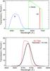 |
Fig. 1 Effective transmission of the VYSOS6 filters convolved with the quantum efficiency of the ALTA U16M CCD camera (top). The position of the narrow-band [SII] 6721 Å filter (red line) and the simulated redshifted Gaussian-shaped Hα emission line using the parameters obtained by Dietrich et al. (2005) (black line) are shown in the bottom panel. |
2. Observations and data reduction
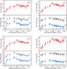 |
Fig. 2 B,r-Sloan and SII-bands light curves for different apertures (5′′upper left, 7.5′′lower left, 15′′upper right and 25′′lower right). The light curves have been corrected for foreground galactic extinction using the values given in Table 1. |
Broad-band Johnson B (4330 Å), Sloan-band r (6230 Å) and the redshifted Hα (SII 6721 ± 30 Å at z = 0.0249) images were obtained with the robotic 15 cm VYSOS6 telescope of the Universitätssternwarte Bochum, located near Cerro Armazones, future location of the ESO Extreme Large Telescope (ELT) in Chile. Monitoring occurred between May 5 and November 18 of 2011, with a median sampling of 3 days.
ESO 399-IG20 lies at redshift z = 0.0249, therefore the Hα emission line falls into the SII 6721 ± 30 Å narrow-band filter. Figure 1 shows the position of the narrow-band with respect to the Hα emission line together with the effective transmission of the other filters used. The Hα line is broader than the SII filter, however, simulations with different asymmetric and perfect symmetric cutting of the high-velocity line wings show negligible systematic effect introduced in the time delay (~2%), even considering the fact of only using one part of the wing profile. This effect will be discussed in depth in a forthcoming contribution (Bruckmann et al., in prep.).
Data reduction was performed using IRAF1, in combination with SCAMP (Bertin 2006) and SWARP (Bertin et al. 2002) routines, in the same manner as described by Haas et al. (2012). Light curves were extracted using different apertures (5′′, 7 5, 15′′ and 25′′) in order to compare and trace the host and AGN contribution. The light curves for the different apertures are shown in Fig. 2. Additionally, for each aperture we determined the level of variability using the fractional flux variation introduced by Rodriguez-Pascual et al. (1997):
  (1)where σ2 is the flux variance of the observations, Δ2 is the mean square uncertainty, and ⟨ f ⟩ is the mean observed flux. The variability statistics is listed in Table 2. Selecting a small aperture (5′′) we are only considering a small portion of the total flux, which remains heavily dependent on the quality of the PSF, whereas bigger apertures (15′′ and 25′′), enclose more contribution of the host-galaxy and the results are more sensitive to sky background contamination resulting in larger uncertainties. We found that 75 around the nucleus is the right size aperture which maximizes the signal-to-noise ratio (S/N) and delivers the lowest absolute scatter for the fluxes. Thus, we use this aperture for the further analysis of the BLR size and AGN luminosity. Although the light curves in Fig. 2 have not yet been corrected for the host galaxy contribution, one can see that the fractional variation (Fvar) and the ratio of the maximum to minimum fluxes (Rmax) are higher in the B-band than in the r-band for which the host-galaxy present a greater contribution. A different case can be seen in the SII light curves, which are mostly dominated by the contribution of the Hα emission line resulting in a higher amplitude of variability. As expected, for bigger apertures the B and r light curves become flatter with Fvar and Rmax smaller due to the larger contribution from the host-galaxy.
Characteristics of ESO 399-IG20.
Light curve variability statistics.
Summary of the photometry results for 75 aperture.
B, r, SII and Hα fluxes corrected by extinction.
Non-variable reference stars located on the same field and with similar brightness as the AGN were used to create the relative light curves in normalized flux units. For the absolute photometry calibration we used reference stars from Landolt (2009) observed on the same nights as the AGN, considering the atmospheric extinction for the nearby site Paranal by Patat et al. (2011) and the recalibrated galactic foreground extinction presented by Schlafly & Finkbeiner (2011) obtained from the Schlegel et al. (1998) dust extinction maps. In Table 1, we give the characteristics of ESO 399-IG20. A summary of the photometric results and the fluxes in all bands are listed in Tables 3 and 4, respectively.
3. Results and discussion
3.1. Light curves and BLR size
The B-band, which is dominated by the AGN continuum, shows a strong flux increase (about 35%) between the beginning and the end of May. Afterwards, the two measurements obtained in June reflect a more gradual increase until a maximum is reached at the end of July. After this maximum, the fluxes decreases gradually (about 20%) until the end of September, and then the light curves become more constant until middle of November. Likewise, the r-band, which is dominated by the continuum but also contains a contribution from the strong Hα emission line, follows the sames features as the B-band light curve, although with a lower amplitude. In contrast to the continuum dominated broad-band light curves, the narrow SII-band light curve exhibits a flux increase which is stretched. For instance the prominent maximum in the B- and r-band at the end of July occurs in the SII-band in August, giving a first approximation for the Hα time delay of 15–20 days. Note that the visual inspection of the r- and B-band light curves does not allow an approximation for the time delay.
As already discussed in previous PRM studies, the narrow-band contains a contribution of the varying continuum, which must be removed before applying cross correlation techniques (Haas et al. 2011; Pozo Nuñez et al. 2012). To determine this contribution, we used the SII and r-band fluxes, previously calibrated to mJy, as is shown with the flux-flux diagram in Fig. 3. The Hα line is strong contributing, on average, about 70% of the total flux enclose in the SII-band, while the continuum contribution (r-band) is about 30%. Following the usual practice of PRM, we construct a synthetic Hα light curve by subtracting a third of the r-band flux (Hα = SII − 0.3 r). The Hα light curve was used afterwards to estimate the time delay. For this purpose, we used the discrete correlation function (DCF, Edelson & Krolik 1988) to cross-correlate the continuum and the synthetic Hα emission line, taking into account possible bin size dependency (Rodriguez-Pascual et al. 1989). The centroid in the cross-correlation of B-band and Hα show a time delay of 18.1 days, while the centroid in the cross-correlation between B-band and SII-band yields a time delay of 15.8 days. However, this is an expected result because of the more pronounced peak at zero lag due to the contamination by the continuum emission in the narrow-band filter. Both cross-correlation functions are shown in Fig. 4. Uncertainties in the time delay were calculated using the flux randomization and random subset selection method (FR/RSS, Peterson et al. 1998, 2004). From the observed light curves we create 2000 randomly selected subset light curves, each containing 63% of the original data points (the other fraction of points are unselected according to Poisson probability). The flux value of each data point was randomly altered consistent with its (normal-distributed) measurement error. We calculated the DCF for the 2000 pairs of subset light curves and the corresponding centroid (Fig. 5). From this cross-correlation error analysis, we measure a median lag of  . Correcting for the time dilation factor (1 + z = 1.0249) we obtain a rest frame lag of 18.2 ± 2.29 days.
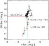 |
Fig. 3 Flux-flux diagram for the SII and r band measured using 7.5′′ aperture. Black dots denote the measurement pair of each night. The straight red and green lines represents the average flux in the SII and r band respectively. The data are as observed and not corrected for galactic foreground extinction. |
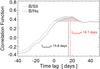 |
Fig. 4 Cross correlation of B and SII light curves (dotted line) and of B and Hα light curves (dashed line). The error range (± 1σ) around the cross correlation was omitted for better viewing. The red and black shaded areas marks the range used to calculate the centroid of the lag (vertical red and black straight lines). |
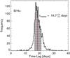 |
Fig. 5 Results of the lag error analysis. The histogram shows the distribution of the centroid lag obtained by cross correlating 2000 flux randomized and randomly selected subset light curves (FR/RSS method). The black area marks the 68% confidence range used to calculate the errors of the centroid (red line). |
An alternative method to estimate the time delay, called Stochastic Process Estimation for AGN Reverberation (SPEAR), has been worked out recently by Zu et al. (2011). Through the modeling of the AGN light curves as a damped random walk (DRW; Zu et al. 2011, 2013 and reference therein), this method appears to be consistent with previous cross-correlation techniques (e.g. Grier et al. 2012, for spectroscopic reverberation data). Using the SPEAR code2 on our light curves, we obtain a time delay of  . After correction for time dilation the rest frame lag τrest = 17.9 ± 1.1 days, in agreement with the results from the DCF method. Figure 6 shows the SPEAR light curve models.
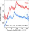 |
Fig. 6 Synthetic Hα and continuum light curves. The solid red and blue lines show the Hα and continuum models estimated by SPEAR respectively. The red and blue area (enclosed by the dashed line) represent the expected variance about the mean light curve model. The original Hα light curve is computed by subtracting a scaled r curve from the SII curve and re-normalizing it to mean = 1 (red dots). The Hα light curve is vertically shifted by 0.2 with respect to the continuum light curve (blue dots) for clarity. |
3.2. Broad-band reverberation mapping approach
Recently, pure broad-band photometric RM has been introduced as an efficient alternative to measure the BLR size in quasars (Chelouche & Daniel 2012). In this method, the emission line is also measured using a broad-band filter, and the removal of the underlying continuum is performed in the correlation domain. The centroid of the lag is obtained by the subtraction of the ACF between the continuum (represented by one broad band filter enclosing only continuum emission) from the CCF between the continuum and the emission line (represented by one broad-band filter that contains a sufficiently strong emission line contribution). This method has been applied for two objects; the low-luminosity AGN NGC 4395 (Edri et al. 2012) and the high-redshift (z = 1.72) luminous MACHO quasar (13.6805.324) (Chelouche et al. 2012); in both cases a successful recovery of the time delay has been reported. Our ESO 399-IG20 has a strong Hα emission line contributing to about 20% to the r-band flux (Fig. 3) and the light curves are well sampled. This makes ESO 399-IG20 an ideal object to perform a further test of the pure broad-band PRM method.
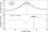 |
Fig. 7 Broad-band RM results. Top: the B-band ACF (dotted line) show a well defined centroid at zero lag (vertical blue line), while the B/r-band CCF shows the same peak at zero lag, a secondary peak at 3 days is also visible (vertical black line). In the same case as the B-band ACF, the r-band ACF (red line) show a peak at zero lag, however, one additionally faint peak is clearly visible between 10–20 days, in comparison with the ACF of the B-band. Bottom: the cross-correlation yields a centroid lag of 15.0 days (vertical black line). The red shaded area marks the range used to calculate the centroid. |
The B-band is mostly dominated by the continuum, and the r-band contains a strong Hα emission line. This allows us to calculate the line-continuum cross-correlation function CCF(τ) = CCFBr(τ) − ACFB(τ) and to obtain the time delay (centroid). As shown in Fig. 7, the B/r cross-correlation exhibits two different peaks, one peak at zero lag (from the auto-correlation of the continuum) and one peak at lag ~3 days. Furthermore, a small but extended enhancement can be seen in the auto-correlation of the r-band at about 10–20 days, in comparison with the ACF of the B-band. This feature can be interpreted as a clear contribution from the Hα emission line to the broad r-band filter. In fact, the cross-correlation shows a broad peak with a lag of 15.0 days as defined by the centroid in Fig. 7. To determine the lag uncertainties, we applied the FR/RSS method. Again from the observed light curves we created 2000 randomly selected subset light curves, each containing 63% of the original data points, and randomly altering the flux value of each data point consistent with its (normal-distributed) measurement error. We calculated the DCF for the 2000 pairs of subset light curves and the corresponding centroid (Fig. 8). This yields a median lag  days. Correcting for time dilation we obtain a rest frame lag τrest = 17.5 ± 3.1 days. This nicely agrees with the results from narrow-band PRM (18.2 ± 2.3 days for the DCF, and 17.9 ± 1.1 days for SPEAR)
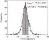 |
Fig. 8 Results of the lag error analysis of CCFBr(τ) − ACFB(τ). The histogram shows the distribution of the centroid lag obtained by cross correlating 2000 flux randomized and randomly selected subset light curves (FR/RSS method). The black shaded area marks the 68% confidence range used to calculate the errors of the centroid (red line). |
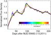 |
Fig. 9 BLR disk/sphere-model. Simulated Hα light curves for a disk-like BLR geometry and different inclinations (4 ≤ i ≤ 30°) are shown in different colors for illustration. The black dotted line is the Hα simulated light curve for a spherical BLR model. A disk-like BLR model with inclination of 6° is able to reproduce the features of the original Hα light curve (black crosses). |
3.3. Modeling the geometry of the broad-line region
We have inferred the geometry of the BLR through the direct modeling of the results obtained from PRM. Following Welsh & Horne (1991), the time delay function for a spherically symmetric geometry of the BLR is: 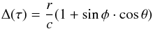 (2)where r is the radius of the spherical shell, φ and θ the respectives angles in the spherical coordinates. While for a Keplerian ring/disk structure the time delay function is:
 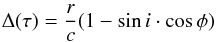 (3)where r is the radius of the ring, i is the inclination (0 ≤ i ≤ 90°) of the axis of the disk with respect to the observer line of sight (0 = face-on, 90 = edge-on) and φ is the azimuthal angle between a point on the disk and the projection of the line of sight onto the disk. The observed continuum light curve (previously interpolated by SPEAR) was convolved with the time-delay function for the respective disk and sphere geometry to simulate the expected Hα light curve. The results of the simulation are shown in Fig. 9.
The Hα light curve for a spherical BLR configuration does not reproduce the observations, however a nearly face-on disk-like BLR geometry with an inclination between 4 to 10° provides an acceptable fit to the original data. To estimate the disk inclination, we performed the χ2 minimizing fitting procedure for a range of inclination angles (Fig. 9). The best fit yields a value of i = 6° ± 3° for a disk-like BLR model with an extension from 16 to 20 light days. For such a nearly face-on BLR the velocity of orbiting broad line gas clouds will appear about a factor ten smaller, mimicking a NLS1.
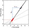 |
Fig. 10 Flux variation gradient diagram of ESO 399-IG20 for |
3.4. AGN luminosity and the Host-subtraction process
Total, host galaxy and AGN fluxes of ESO 399-IG20.
To determine the AGN luminosity free of host galaxy contributions, we applied the flux variation gradient (FVG) method, originally proposed by Choloniewski (1981) and later modified by Winkler et al. (1992). A detailed description of the FVG method on PRM data is presented in Pozo Nuñez et al. (2012), and here we give a brief outline. In this method the fluxes obtained through different filters and same apertures are plotted in a flux-flux diagram. The fluxes follow a linear slope representing the AGN color, while the slope of the nuclear host galaxy contribution (including the contribution from the narrow line region (NLR)) lies in a well defined range ( , for 83 aperture and redshift z < 0.03, Sakata et al. 2010). The AGN slope is determined through linear regression analysis. The intersection of the AGN slope with the host galaxy range yields the actual host galaxy contribution at the time of the monitoring campaign. Figure 10 shows the FVG diagram for the B and r fluxes (corrected for galactic foreground extinction) obtained during the same nights and through
  aperture. Additionally, FVGs were evaluated for different apertures, as shown in Fig. 11. As already noted in Sect. 2, a big fraction of the total flux is lost in the small 5′′ aperture, hence, the results are more sensitive to a possible underestimation of the real AGN and host galaxy contribution. Furthermore, one may expect that for larger apertures the fluxes will lie closer to the range for the host galaxy slope, however, it appears that the host galaxy is intrinsically strong and very blue, closer to the nucleus and in the outer parts. As for the analysis of the light curves we here use the results for the 75 aperture.
Averaging over the intersection area between the AGN and the host galaxy slopes, we obtain a mean host galaxy flux of (0.95 ± 0.18) mJy in B and (2.51 ± 0.20) mJy in r. During our monitoring campaign the host galaxy subtracted AGN fluxes range between 2.29 and 2.71 and between 2.14 and 2.58 mJy in the B and r band, respectively. These fluxes are represented by the blue dotted lines in Fig. 10. From this range we interpolate the host-subtracted monochromatic AGN flux at restframe 5100 Å F5100 = 2.66 ± 0.22 × 10⁻¹⁵ erg s-1 cm-2 Å-1. For the interpolation we assumed a power law spectral energy distribution (SED) (Fν ∝ να) with an spectral index α = log (fBAGN/frAGN)/log (νB/νr), where νB and νr are the effective frequencies in the B and r bands, respectively. The error was determined by interpolation between the ranges of the AGN fluxes ± σ in both filters. At the distance of 102 Mpc this yields a host-subtracted AGN luminosity at 5100 Å LAGN = (1.69 ± 0.25) × 1043 erg s-1. The total fluxes, host galaxy subtracted AGN fluxes and the AGN luminosity are listed in Table 5.
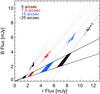 |
Fig. 11 Flux variation gradient diagram of ESO 399-IG20 for different apertures. The fluxes obtained through |
3.5. The BLR size-luminosity relationship
Estimates of the BLR size and host-galaxy subtracted AGN luminosity in the literature have been derived from several spectroscopic RM campaigns and through host-galaxy modeling using high-resolution images from HST. In consequence, the relationship between the Hβ BLR size and the luminosity (5100 Å) RBLR ∝ Lα (Kaspi et al. 2000) has been improved considerably with the most recent slope of α = 0.519 (Bentz et al. 2009). Although to date this relationship has been corroborated for 38 AGNs, still there exist objects with large uncertainties in both measurements. In order to improve the statistic, it is of interest to see the position for this new Seyfert 1 galaxy on the BLR-Luminosity relationship. In order to obtain the Hβ BLR radius, we used the weighted mean ratio for the time lag τ(Hα):τ(Hβ):1.54:1.00, obtained recently by Bentz et al. (2010) from the Lick AGN Monitoring Program of 11 low-luminosity AGN. Therefore, the Hα lag of 18.2 days translates into an Hβ lag of 11.8 days. Figure 12 shows the position of ESO 399-IG20 on the RBLR-LAGN diagram. The data are taken from Bentz et al. (2009) and here we include the most recent results for particular objects obtained from spectroscopic RM by Denney et al. (2010), Doroshenko et al. (2012) and Grier et al. (2012) respectively.
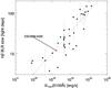 |
Fig. 12 RBLR versus L, using data from Bentz et al. (2009), Denney et al. (2010), Doroshenko et al. (2012) and Grier et al. (2012). As a red dot we included our results for ESO 399-IG20. Shown is a zoomed portion containing ESO 399-IG20. The solid dotted line show a fitted slope α = 0.519. ESO 399-IG20 lies close to the expected slope. |
4. Summary and conclusions
We presented new photometric reverberation mapping results for the Seyfert 1 galaxy ESO 399-IG20. We determined the broad line region size, the basic geometry of the BLR and the host-subtracted AGN luminosity. The results are:
-
1.
The cross-correlation of the Hα emission line measured in a narrow-band filter with the optical continuum light curve yields a rest-frame time delay τrest = 18.2 ± 2.29 days. We explored the SPEAR method, and – given that Hα contributes about 15–20% to the r-band – also the capabilities of pure broad-band photometric reverberation mapping. The SPEAR method yields a rest-frame time delay of τrest = 17.9 ± 1.1 days, while the pure broad-band PRM method yields τrest = 17.5 ± 3.1 days. The results indicate that, within the errors, the three methods are in good agreement.
-
2.
We constrained the basic geometry of the BLR by comparing simulated light curves, using the size determined for the BLR, to the observed Hα light curve. The pronounced and sharp variability features in both the continuum and emission line light curves allow us to exclude a spherical BLR geometry. We found that the BLR has a disk-like shape with an inclination of i = 6 ± 3° and an extension from 16 to 20 light days. This nearly face-on BLR can explain the appearance of ESO 399-IG20 as a narrow-line Seyfert-1 galaxy.
-
3.
We successfully separated the host-galaxy contribution from the total flux through the flux variation gradient method (FVG). The average host-galaxy subtracted AGN luminosity of ESO 399-IG20 at the time of our monitoring campaign is LAGN = (1.69 ± 0.25) × 1043 erg s-1. In the BLR size – AGN luminosity diagram ESO 399-IG20 lies close to the best fit of the relation.
These results document the efficiency and accuracy of photometric reverberation mapping for determining the AGN luminosity, the BLR size and the potential to constrain even the BLR geometry.
IRAF is distributed by the National Optical Astronomy Observatory, which is operated by the Association of Universities for Research in Astronomy (AURA) under cooperative agreement with the National Science Foundation.
Acknowledgments
This publication is supported as a project of the Nordrhein-Westfälische Akademie der Wissenschaften und der Künste in the framework of the academy program by the Federal Republic of Germany and the state Nordrhein-Westfalen. The observations on Cerro Armazones benefitted from the care of the guardians Hector Labra, Gerardo Pino, Roberto Munoz, and Francisco Arraya. This research has made use of the NASA/IPAC Extragalactic Database (NED) which is operated by the Jet Propulsion Laboratory, California Institute of Technology, under contract with the National Aeronautics and Space Administration. This research has made use of the SIMBAD database, operated at CDS, Strasbourg, France. We thank the anonymous referee for his comments and careful review of the manuscript.
References
- Bentz, M. C., Peterson, B. M., Netzer, H., Pogge, R. W., & Vestergaard, M. 2009, ApJ, 697, 160 [Google Scholar]
- Bentz, M. C., Walsh, J. L., Barth, A. J., et al. 2010, ApJ, 716, 993 [NASA ADS] [CrossRef] [Google Scholar]
- Bertin, E. 2006, Astronomical Data Analysis Software and Systems XV, 351, 112 [NASA ADS] [Google Scholar]
- Bertin, E., Mellier, Y., Radovich, M., et al. 2002, Astronomical Data Analysis Software and Systems XI, 281, 228 [NASA ADS] [Google Scholar]
- Blandford, R. D., & McKee, C. F. 1982, ApJ, 255, 419 [NASA ADS] [CrossRef] [EDP Sciences] [Google Scholar]
- Chelouche, D., & Daniel, E. 2012, ApJ, 747, 62 [NASA ADS] [CrossRef] [Google Scholar]
- Chelouche, D., Daniel, E., & Kaspi, S. 2012, ApJ, 750, L43 [NASA ADS] [CrossRef] [Google Scholar]
- Choloniewski, J. 1981, Acta Astron., 31, 293 [NASA ADS] [Google Scholar]
- Davidson, K., & Netzer, H. 1979, Rev. Mod. Phys., 51, 715 [NASA ADS] [CrossRef] [Google Scholar]
- Denney, K. D., Peterson, B. M., Pogge, R. W., et al. 2010, ApJ, 721, 715 [NASA ADS] [CrossRef] [Google Scholar]
- Dietrich, M., Crenshaw, D. M., & Kraemer, S. B. 2005, ApJ, 623, 700 [NASA ADS] [CrossRef] [Google Scholar]
- Doroshenko, V. T., Sergeev, S. G., Klimanov, S. A., Pronik, V. I., & Efimov, Y. S. 2012, MNRAS, 426, 416 [NASA ADS] [CrossRef] [Google Scholar]
- Edelson, R. A., & Krolik, J. H. 1988, ApJ, 333, 646 [NASA ADS] [CrossRef] [Google Scholar]
- Edri, H., Rafter, S. E., Chelouche, D., Kaspi, S., & Behar, E. 2012, ApJ, 756, 73 [NASA ADS] [CrossRef] [Google Scholar]
- Grier, C. J., Peterson, B. M., Pogge, R. W., et al. 2012, ApJ, 755, 60 [NASA ADS] [CrossRef] [Google Scholar]
- Haas, M., Chini, R., Ramolla, M., et al. 2011, A&A, 535, A73 [NASA ADS] [CrossRef] [EDP Sciences] [Google Scholar]
- Haas, M., Hackstein, M., Ramolla, M., et al. 2012, Astron. Nachr., 333, 706 [NASA ADS] [Google Scholar]
- Kaspi, S., Smith, P. S., Maoz, D., Netzer, H., & Jannuzi, B. T. 1996, ApJ, 471, L75 [NASA ADS] [CrossRef] [Google Scholar]
- Kaspi, S., Smith, P. S., Netzer, H., et al. 2000, ApJ, 533, 631 [NASA ADS] [CrossRef] [Google Scholar]
- Kaspi, S., Brandt, W. N., Maoz, D., et al. 2007, ApJ, 659, 997 [NASA ADS] [CrossRef] [Google Scholar]
- Koratkar, A. P., & Gaskell, C. M. 1991, ApJ, 370, L61 [NASA ADS] [CrossRef] [Google Scholar]
- Landolt, A. U. 2009, AJ, 137, 4186 [NASA ADS] [CrossRef] [Google Scholar]
- McGill, K. L., Woo, J.-H., Treu, T., & Malkan, M. A. 2008, ApJ, 673, 703 [NASA ADS] [CrossRef] [Google Scholar]
- Netzer, H., & Peterson, B. M. 1997, Astron. Time Ser., 218, 85 [NASA ADS] [Google Scholar]
- Patat, F., Moehler, S., O’Brien, K., et al. 2011, A&A, 527, A91 [NASA ADS] [CrossRef] [EDP Sciences] [Google Scholar]
- Peterson, B. M. 1993, PASP, 105, 247 [NASA ADS] [CrossRef] [Google Scholar]
- Peterson, B. M., & Wandel, A. 1999, ApJ, 521, L95 [NASA ADS] [CrossRef] [Google Scholar]
- Peterson, B. M., Wanders, I., Horne, K., et al. 1998, PASP, 110, 660 [NASA ADS] [CrossRef] [Google Scholar]
- Peterson, B. M., Ferrarese, L., Gilbert, K. M., et al. 2004, ApJ, 613, 682 [NASA ADS] [CrossRef] [Google Scholar]
- Pozo Nuñez, F., Ramolla, M., Westhues, C., et al. 2012, A&A, 545, A84 [NASA ADS] [CrossRef] [EDP Sciences] [Google Scholar]
- Rodriguez-Pascual, P. M., Santos-Lleo, M., & Clavel, J. 1989, A&A, 219, 101 [NASA ADS] [Google Scholar]
- Rodriguez-Pascual, P. M., Alloin, D., Clavel, J., et al. 1997, ApJS, 110, 9 [NASA ADS] [CrossRef] [Google Scholar]
- Sakata, Y., Minezaki, T., Yoshii, Y., et al. 2010, ApJ, 711, 461 [NASA ADS] [CrossRef] [Google Scholar]
- Schlafly, E. F., & Finkbeiner, D. P. 2011, ApJ, 737, 103 [NASA ADS] [CrossRef] [Google Scholar]
- Schlegel, D. J., Finkbeiner, D. P., & Davis, M. 1998, ApJ, 500, 525 [NASA ADS] [CrossRef] [Google Scholar]
- Véron-Cetty, M.-P., & Véron, P. 2010, A&A, 518, A10 [NASA ADS] [CrossRef] [EDP Sciences] [Google Scholar]
- Vestergaard, M., Denney, K., Fan, X., et al. 2011, Narrow-Line Seyfert 1 Galaxies and their Place in the Universe, [Google Scholar]
- Wandel, A., Peterson, B. M., & Malkan, M. A. 1999, ApJ, 526, 579 [NASA ADS] [CrossRef] [Google Scholar]
- Welsh, W. F., & Horne, K. 1991, ApJ, 379, 586 [NASA ADS] [CrossRef] [Google Scholar]
- Winkler, H. 1997, MNRAS, 292, 273 [NASA ADS] [CrossRef] [Google Scholar]
- Winkler, H., Glass, I. S., van Wyk, F., et al. 1992, MNRAS, 257, 659 [NASA ADS] [Google Scholar]
- Zu, Y., Kochanek, C. S., & Peterson, B. M. 2011, ApJ, 735, 80 [NASA ADS] [CrossRef] [Google Scholar]
- Zu, Y., Kochanek, C. S., Kozłowski, S., & Udalski, A. 2013, ApJ, 765, 106 [NASA ADS] [CrossRef] [Google Scholar]
All Tables
All Figures
|
Fig. 1 Effective transmission of the VYSOS6 filters convolved with the quantum efficiency of the ALTA U16M CCD camera (top). The position of the narrow-band [SII] 6721 Å filter (red line) and the simulated redshifted Gaussian-shaped Hα emission line using the parameters obtained by Dietrich et al. (2005) (black line) are shown in the bottom panel. |
| In the text | |
|
Fig. 2 B,r-Sloan and SII-bands light curves for different apertures (5′′upper left, 7.5′′lower left, 15′′upper right and 25′′lower right). The light curves have been corrected for foreground galactic extinction using the values given in Table 1. |
| In the text | |
|
Fig. 3 Flux-flux diagram for the SII and r band measured using 7.5′′ aperture. Black dots denote the measurement pair of each night. The straight red and green lines represents the average flux in the SII and r band respectively. The data are as observed and not corrected for galactic foreground extinction. |
| In the text | |
|
Fig. 4 Cross correlation of B and SII light curves (dotted line) and of B and Hα light curves (dashed line). The error range (± 1σ) around the cross correlation was omitted for better viewing. The red and black shaded areas marks the range used to calculate the centroid of the lag (vertical red and black straight lines). |
| In the text | |
|
Fig. 5 Results of the lag error analysis. The histogram shows the distribution of the centroid lag obtained by cross correlating 2000 flux randomized and randomly selected subset light curves (FR/RSS method). The black area marks the 68% confidence range used to calculate the errors of the centroid (red line). |
| In the text | |
|
Fig. 6 Synthetic Hα and continuum light curves. The solid red and blue lines show the Hα and continuum models estimated by SPEAR respectively. The red and blue area (enclosed by the dashed line) represent the expected variance about the mean light curve model. The original Hα light curve is computed by subtracting a scaled r curve from the SII curve and re-normalizing it to mean = 1 (red dots). The Hα light curve is vertically shifted by 0.2 with respect to the continuum light curve (blue dots) for clarity. |
| In the text | |
|
Fig. 7 Broad-band RM results. Top: the B-band ACF (dotted line) show a well defined centroid at zero lag (vertical blue line), while the B/r-band CCF shows the same peak at zero lag, a secondary peak at 3 days is also visible (vertical black line). In the same case as the B-band ACF, the r-band ACF (red line) show a peak at zero lag, however, one additionally faint peak is clearly visible between 10–20 days, in comparison with the ACF of the B-band. Bottom: the cross-correlation yields a centroid lag of 15.0 days (vertical black line). The red shaded area marks the range used to calculate the centroid. |
| In the text | |
|
Fig. 8 Results of the lag error analysis of CCFBr(τ) − ACFB(τ). The histogram shows the distribution of the centroid lag obtained by cross correlating 2000 flux randomized and randomly selected subset light curves (FR/RSS method). The black shaded area marks the 68% confidence range used to calculate the errors of the centroid (red line). |
| In the text | |
|
Fig. 9 BLR disk/sphere-model. Simulated Hα light curves for a disk-like BLR geometry and different inclinations (4 ≤ i ≤ 30°) are shown in different colors for illustration. The black dotted line is the Hα simulated light curve for a spherical BLR model. A disk-like BLR model with inclination of 6° is able to reproduce the features of the original Hα light curve (black crosses). |
| In the text | |
|
Fig. 10 Flux variation gradient diagram of ESO 399-IG20 for |
| In the text | |
|
Fig. 11 Flux variation gradient diagram of ESO 399-IG20 for different apertures. The fluxes obtained through |
| In the text | |
|
Fig. 12 RBLR versus L, using data from Bentz et al. (2009), Denney et al. (2010), Doroshenko et al. (2012) and Grier et al. (2012). As a red dot we included our results for ESO 399-IG20. Shown is a zoomed portion containing ESO 399-IG20. The solid dotted line show a fitted slope α = 0.519. ESO 399-IG20 lies close to the expected slope. |
| In the text | |
Current usage metrics show cumulative count of Article Views (full-text article views including HTML views, PDF and ePub downloads, according to the available data) and Abstracts Views on Vision4Press platform.
Data correspond to usage on the plateform after 2015. The current usage metrics is available 48-96 hours after online publication and is updated daily on week days.
Initial download of the metrics may take a while.