| Issue |
A&A
Volume 552, April 2013
|
|
|---|---|---|
| Article Number | A70 | |
| Number of page(s) | 10 | |
| Section | Planets and planetary systems | |
| DOI | https://doi.org/10.1051/0004-6361/201220626 | |
| Published online | 27 March 2013 | |
A giant planet beyond the snow line in microlensing event OGLE-2011-BLG-0251
1
European Southern Observatory, Karl-Schwarzschild Straße 2, 85748
Garching bei München,
Germany
2
Las Cumbres Observatory Global Telescope Network,
6740 Cortona Drive, Suite 102,
Goleta, CA
93117,
USA
3
Department of Physics, Institute for Astrophysics, Chungbuk
National University, 371-763
Cheongju,
Korea
4
Warsaw University Observatory, Al. Ujazdowskie 4, 00-478
Warszawa,
Poland
5
Divisão de Astrofisica, Instituto Nacional de Pesquisas
Espeaciais, Avenida dos
Astronauntas, 1758 Sao José dos Campos, 12227-010
SP,
Brazil
6
School of Chemical and Physical Sciences, Victoria
University, Wellington, New Zealand
7
Niels Bohr Institute, University of Copenhagen,
Juliane Maries vej 30,
2100
Copenhagen,
Denmark
8
Centre for Star and Planet Formation, Geological
Museum, Øster Voldgade
5, 1350
Copenhagen,
Denmark
9
Qatar Foundation, PO Box 5825, Doha, Qatar
10
Dipartimento di Fisica “E.R Caianiello”, Università di
Salerno, via Ponte Don
Melillo, 84084
Fisciano,
Italy
11
Istituto Nazionale di Fisica Nucleare,
Sezione di Napoli,
Italy
12
SUPA School of Physics & Astronomy, University of St
Andrews, North
Haugh, St Andrews,
KY16 9SS,
UK
13
Deutsches SOFIA Institut, Universität Stuttgart,
Pfaffenwaldring 31,
70569
Stuttgart,
Germany
14
SOFIA Science Center, NASA Ames Research Center, Mail Stop
N211-3, Moffett Field
CA
94035,
USA
15
Istituto Internazionale per gli Alti Studi Scientifici
(IIASS), Vietri Sul
Mare ( SA),
Italy
16
Institut für Astrophysik, Georg-August-Universität,
Friedrich-Hund-Platz 1,
37077
Göttingen,
Germany
17
Korea Astronomy and Space Science Institute,
305-348
Daejeon,
Korea
18
National Astronomical Observatories/Yunnan Observatory, Joint
laboratory for Optical Astronomy, Chinese Academy of Sciences,
650011
Kunming, PR
China
19
Department of Physics and Astronomy, Aarhus
University, Ny Munkegade
120, 8000
Århus C,
Denmark
20
Armagh Observatory, College Hill, Armagh, BT61 9DG, Northern Ireland, UK
21
Danmarks Tekniske Universitet, Institut for Rumforskning og
-teknologi, Juliane Maries Vej
30, 2100
København,
Denmark
22
Jodrell Bank Centre for Astrophysics, University of
Manchester, Oxford
Road, Manchester,
M13 9PL,
UK
23
Max Planck Institute for Astronomy, Königstuhl 17, 69117
Heidelberg,
Germany
24
Department of Astronomy, Ohio State University,
140 West 18th Avenue,
Columbus, OH
43210,
USA
25
Department of Physics, Sharif University of
Technology, PO Box
11155–9161, Tehran,
Iran
26
Perimeter Institute for Theoretical Physics,
31 Caroline St. N.,
Waterloo ON, N2L 2Y5, Canada
27
Institut d’Astrophysique et de Géophysique,
Allée du 6 Août 17, Sart Tilman, Bât.
B5c, 4000
Liège,
Belgium
28
Space Telescope Science Institute, 3700 San Martin Drive, Baltimore, MD
21218,
USA
29
INFN, Gruppo Collegato di Salerno, Sezione di Napoli,
Italy
30
European Southern Observatory (ESO), Alonso de Cordova 3107, Casilla 19001,
Santiago 19,
Chile
31
Max Planck Institute for Solar System Research,
Max-Planck-Str. 2, 37191
Katlenburg-Lindau,
Germany
32
Astrophysics Group, Keele University, Staffordshire, ST5 5BG, UK
33
Astronomisches Rechen-Institut, Zentrum für Astronomie der
Universität Heidelberg (ZAH), Mönchhofstr. 12-14, 69120
Heidelberg,
Germany
34
Institute of Astronomy, University of Cambridge,
Madingley Road, Cambridge
CB3 0HA,
UK
35
Alsubais Establishment for Scientific Studies,
Doha,
Qatar
36
Astrophysics Research Institute, Liverpool John Moores
University, Twelve Quays House,
Egerton Wharf, Birkenhead, Wirral., CH41
1LD, UK
37
School of Mathematical Sciences, Queen Mary, University of
London, Mile End
Road, London
E1 4NS,
UK
38
Vintage Lane Observatory, 83 Vintage Lane, RD3, Blenheim, New
Zealand
39
Auckland Observatory, 670 Manukau Rd, Royal Oak 1023, Auckland, New
Zealand
40
Dept. of Physics and Astronomy, Texas A&M University
College Station, TX
77843-4242, USA
41
Possum Observatory, Patutahi, Gisbourne, New Zealand
42
Farm Cove Observatory, Centre for Backyard Astrophysics,
Pakuranga, Auckland,
New Zealand
43
Institute for Radiophysics and SpaceResearch, AUT
University, Auckland,
New Zealand
44
Dept. of Astronomy and Space Science, Chungnam
University, Korea
45
Departamento de Astronomiá y Astrofísica, Universidad de
Valencia, 46100
Burjassot, Valencia, Spain
46
UPMC-CNRS, UMR7095, Institut d’Astrophysique de
Paris, 98bis boulevard
Arago, 75014
Paris,
France
47
University of Canterbury, Dept. of Physics and
Astronomy, Private Bag
4800, 8020
Christchurch, New
Zealand
48
McDonald Observatory, 16120 St Hwy Spur 78 #2, Fort Davis, Tx
79734,
USA
49
University of the Free State, Faculty of Natural and Agricultural
Sciences, Dept. of Physics, PO Box
339, 9300
Bloemfontein, South
Africa
50
School of Math and Physics, University of Tasmania,
Private Bag 37, GPO Hobart,
7001
Tasmania,
Australia
51
Institute of Geophysics and Planetary Physics (IGPP), L-413,
Lawrence Livermore National Laboratory, PO Box 808, Livermore, CA
94551,
USA
52
Université de Toulouse, UPS-OMP, IRAP,
31400
Toulouse,
France
53
CNRS, IRAP, 14
avenue Edouard Belin, 31400
Toulouse,
France
54
Physics Department, Faculty of Arts and Sciences, University of
Rijeka, Omladinska
14, 51000
Rijeka,
Croatia
55
Technical University of Vienna, Department of
Computing, Wiedner Hauptstrasse
10, Vienna,
Austria
56
NASA Exoplanet Science Institute, Caltech, MS 100-22, 770 S. Wilson Ave.,
Pasadena, CA
91125,
USA
57
Perth Observatory, Walnut Road, Bickley,
6076
Perth,
Australia
58
South African Astronomical Observatory,
PO Box 9, Observatory
7935, South
Africa
59
Solar-Terrestrial Environment Laboratory, Nagoya
University, 464-8601
Nagoya,
Japan
60
Dept. of Physics, University of Notre Dame,
Notre Dame, IN
46556,
USA
61
Institute of Information and Mathematical Sciences, Massey
University, Private Bag 102-904,
North Shore Mail Centre, Auckland, New Zealand
62
Dept. of Physics, University of Auckland,
Private Bag 92019, Auckland, New
Zealand
63
Okayama Astrophysical Observatory, National Astronomical
Observatory of Japan, Asakuchi, 719-0232
Okayama,
Japan
64
Mt. John Observatory, PO Box 56, 8770
Lake Tekapo, New
Zealand
65
Dept. of Physics, Konan University, Nishiokamoto 8-9-1, 658-8501
Kobe,
Japan
66
Nagano National College of Technology,
381-8550
Nagano,
Japan
67
Tokyo Metropolitan College of Industrial Technology,
116-8523
Tokyo,
Japan
68
Dept. of Earth and Space Science, Graduate School of Science,
Osaka University, 1-1
Machikaneyama-cho, Toyonaka, 560-0043
Osaka,
Japan
69
Universidad de Concepción, Departamento de
Astronomia, Casilla
160–C, Concepción,
Chile
Received:
24
October
2012
Accepted:
1
March
2013
Abstract
Aims. We present the analysis of the gravitational microlensing event OGLE-2011-BLG-0251. This anomalous event was observed by several survey and follow-up collaborations conducting microlensing observations towards the Galactic bulge.
Methods. Based on detailed modelling of the observed light curve, we find that the lens is composed of two masses with a mass ratio q = 1.9 × 10⁻³. Thanks to our detection of higher-order effects on the light curve due to the Earth’s orbital motion and the finite size of source, we are able to measure the mass and distance to the lens unambiguously.
Results. We find that the lens is made up of a planet of mass 0.53 ± 0.21 MJ orbiting an M dwarf host star with a mass of 0.26 ± 0.11 M⊙. The planetary system is located at a distance of 2.57 ± 0.61 kpc towards the Galactic centre. The projected separation of the planet from its host star is d = 1.408 ± 0.019, in units of the Einstein radius, which corresponds to 2.72 ± 0.75 AU in physical units. We also identified a competitive model with similar planet and host star masses, but with a smaller orbital radius of 1.50 ± 0.50 AU. The planet is therefore located beyond the snow line of its host star, which we estimate to be around ~1−1.5 AU.
Key words: gravitational lensing: weak / planets and satellites: detection / planetary systems / Galaxy: bulge
Corresponding authors: e-mail: This email address is being protected from spambots. You need JavaScript enabled to view it. ; This email address is being protected from spambots. You need JavaScript enabled to view it.
Royal Society University Research Fellow.
© ESO, 2013
1. Introduction
Gravitational microlensing is one of the methods that allow us to probe the populations of extrasolar planets in the Milky Way, and has now led to the discoveries of 16 planets1, several of which could not have been detected with other techniques (e.g. Beaulieu et al. 2006; Gaudi et al. 2008; Muraki et al. 2011). In particular, microlensing events can reveal cool, low-mass planets that are difficult to detect with other methods. Although this method presents several observational and technical challenges, it has recently led to several significant scientific results. Sumi et al. (2011) analysed short time-scale microlensing events and concluded that these events were produced by a population of Jupiter-mass free-floating planets, and were able to estimate the number of such objects in the Milky Way. Cassan et al. (2012) used 6 years of observational data from the PLANET collaboration to build on the work of Gould et al. (2010) and Sumi et al. (2011), and derived a cool planet mass function, suggesting that, on average, the number of planets per star is expected to be more than 1.
Modelling gravitational microlensing events has been and remains a significant challenge, due to a complex parameter space and computationally demanding calculations. Recent developments in modelling methods (e.g. Cassan 2008; Kains et al. 2009, 2012; Bennett 2010; Ryu et al. 2010; Bozza et al. 2012), however, have allowed microlensing observing campaigns to optimise their strategies and scientific output, thanks to real-time modelling providing prompt feedback to observers as to the possible nature of ongoing events.
In this paper we present an analysis of microlensing event OGLE-2011-BLG-0251, an anomalous event discovered during the 2011 season by the OGLE collaboration and observed intensively by follow-up teams. In Sect. 2, we briefly summarise the basics of relevant microlensing formalism, while we discuss our data and reduction in Sect. 3. Our modelling approach and results are outlined in Sect. 4; we translate this into physical parameters of the lens system in Sect. 5 and discuss the properties of the planetary system we infer.
2. Microlensing formalism
Microlensing can be observed when a source becomes sufficiently aligned with a lens along
the line of sight that the deflection of the source light by the lens is significant. A
characteristic separation at which this occurs is the Einstein ring radius. When a single
point source approaches a single point lens of mass M with a projected
source-lens separation u, the source brightness is magnified following a
symmetric “point source-point lens” (PSPL) pattern which can be parameterised with an impact
parameter u0 and a timescale tE,
both expressed in units of the angular Einstein radius (Einstein 1936),  (1)where G is
the gravitational constant, c is the speed of light,
and DS and DL are the distances to
the source and the lens, respectively, from the observer. The timescale is then
tE = θE/μ,
where μ is the lens-source relative proper motion. Therefore the observable
tE is a degenerate function of
M,DL and the source’s transverse velocity
v⊥, assuming that DS is known.
However, measuring certain second-order effects in microlensing light curves such as the
parallax due to the Earth’s orbit allows us to break this degeneracy and therefore measure
the properties of the lensing system directly.
(1)where G is
the gravitational constant, c is the speed of light,
and DS and DL are the distances to
the source and the lens, respectively, from the observer. The timescale is then
tE = θE/μ,
where μ is the lens-source relative proper motion. Therefore the observable
tE is a degenerate function of
M,DL and the source’s transverse velocity
v⊥, assuming that DS is known.
However, measuring certain second-order effects in microlensing light curves such as the
parallax due to the Earth’s orbit allows us to break this degeneracy and therefore measure
the properties of the lensing system directly.
When the lens is made up of two components, the magnification pattern can follow many
different morphologies, because of singularities in the lens equation. These lead to source
positions, along closed caustic curves, where the lensing magnification is
formally infinite for point sources, although the finite size of sources means that, in
practice, the magnification gradient is large rather than infinite. A point-source
binary-lens (PSBL) light curve is often described by 6 parameters: the time at which the
source passes closest to the centre of mass of the binary lens,
t0, the Einstein radius crossing time,
tE, the minimum impact parameter
u0, which are also used to describe PSPL light curves, as well
as the source’s trajectory angle α with respect to the lens components, the
separation between the two mass components, d, and their mass ratio
q. Finite source size effects can be parameterised in a number of ways,
usually by defining the angular size of the source ρ ∗ in units
of θE:  (2)where
θ ∗ is the angular size of the source in standard units.
(2)where
θ ∗ is the angular size of the source in standard units.
Data sets for OGLE-2011-BLG-0251, with the number of data points for each telescope/filter combination.
3. Observational data
The microlensing event OGLE-2011-BLG-0251 was discovered by the Optical Gravitational Lens Experiment (OGLE) collaboration’s Early Warning System (Udalski 2003) as part of the release of the first 431 microlensing alerts following the OGLE-IV upgrade. The source of the event has equatorial coordinates α = 17h38m14.18s and δ = −27°08′10.1′′ (J2000.0), or Galactic coordinates of (l,b) = (0.670°,2.334°). Anomalous behaviour was first detected and alerted on August 9, 2011 (HJD ~ 2 455 782.5) thanks to real-time modelling efforts by various follow-up teams that were observing the event, but by that time a significant part of the anomaly had already passed, with sub-optimal coverage due to unfavourable weather conditions. The anomaly appears as a two-day feature spanning HJD = 2 455 779.5 to 2 455 781.5, just before the time of closest approach t0. Despite difficult weather and moonlight conditions, the anomaly was securely covered by data from five follow-up telescopes in Brazil (μFUN Pico dos Dias), Chile (MiNDSTEp Danish 1.54 m) New Zealand (μFUN Vintage Lane, and MOA Mt. John B&C), and the Canary Islands (RoboNet Liverpool Telescope).
The descending part of the light curve also suffered from the bright Moon, with the source ~5 degrees from the Moon at ~85% of full illumination, leading to high background counts in images and more scatter in the reduced data. We opted not to include data from Mt. Canopus 1 m telescope in the modelling because of technical issues at the telescope affecting the reliability of the images, and also excluded the I-band data from CTIO because they also suffer from large scatter, probably due to the proximity of the bright full Moon to the source.
The data set amounts to 3738 images from 13 sites, from the OGLE survey team, the MiNDSTEp consortium, the RoboNet team, as well as the μFUN, PLANET and MOA collaborations in the I,V and R bands, as well as some unfiltered data; data sets are summarised in Table 1 and the light curve is shown in Fig. 1. We reduced all data using the difference imaging pipeline DanDIA (Bramich 2008; Bramich et al. 2013), except for the OGLE data, which was reduced by the OGLE team with their optimised offline pipeline.
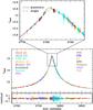 |
Fig. 1 Light curve of OGLE-2011-BLG-0251. Data points are plotted with 1-σ error bars, and the upper panel shows a zoom around the perturbation region near the peak |
For each data set, we applied an error bar rescaling factors a and
b to normalise error bars with respect to our best-fit model (see
Sect. 4), using the simple scaling relation
 where
where  is the rescaled
error bar of the ith data point and
σi is the original error bar (e.g. Bachelet et al. 2012). The error bar rescaling factors for
each data set is given in Table 1. We did not exclude
outliers from our data sets, unless we had reasons to believe that an outlier had its origin
in a bad observation, or in issues with the data reduction pipeline.
is the rescaled
error bar of the ith data point and
σi is the original error bar (e.g. Bachelet et al. 2012). The error bar rescaling factors for
each data set is given in Table 1. We did not exclude
outliers from our data sets, unless we had reasons to believe that an outlier had its origin
in a bad observation, or in issues with the data reduction pipeline.
4. Modelling
We modelled the light curve of the event using a Markov chain Monte Carlo (MCMC) algorithm with adaptive step size. We first used the “standard” PSBL parameterisation in our modelling, whereby a binary-lens light curve can be described by 6 parameters: those given in Sect. 2, ignoring the second-order ρ ∗ parameter described in that section. For all models and configurations we searched the parameter space for solutions with both a positive and a negative impact parameter u0.
We started without including second-order effects of the source having a finite size or parallax due to the orbital motion of Earth around the Sun, and then added these separately in subsequent modelling runs by fitting the source size parameter ρ ∗ , as defined in Sect. 2, and the parallax parameters described below. Both effects led to a large decrease in the χ2 statistic of the model (>1000), which could not be explained only by the extra number of parameters.
For the finite-source effect, we additionally considered the limb-darkening variation of
the source star surface brightness by modelling the surface-brightness profile as
![Mathematical equation: \begin{equation} \label{eq:lld} I_{\psi, \lambda} = I_{0, \lambda} [1 - c_l\,(1-\cos\psi)], \end{equation}](/articles/aa/full_html/2013/04/aa20626-12/aa20626-12-eq54.png) (3)where
I0,ψ is the brightness at the centre of the
source, and ψ is the angle between a normal to the surface and the line of
sight. We adopt the limb-darkening coefficients based on the source type determined from the
dereddened colour and brightness (see Sect. 5.1). The
values of the adopted coefficients are
cV = 0.073,cI = 0.624,cR = 0.542,
based on the catalogue of Claret (2000).
(3)where
I0,ψ is the brightness at the centre of the
source, and ψ is the angle between a normal to the surface and the line of
sight. We adopt the limb-darkening coefficients based on the source type determined from the
dereddened colour and brightness (see Sect. 5.1). The
values of the adopted coefficients are
cV = 0.073,cI = 0.624,cR = 0.542,
based on the catalogue of Claret (2000).
Finally, in a third round of modelling, we included both the effects of parallax and finite source size (“ESBL + parallax”). Including these effects together led to a significant improvement of the fit, with Δχ2 > 500 compared to the fits in which those effects were added separately. Computing the f-statistic (see e.g. Lupton 1993) for this difference tells us that the probability of this difference occurring solely due to the number of degrees of freedom decreasing by 1 or 2 is highly unlikely. Our best-fit ESBL + parallax model is shown in Fig. 1.
To model the effect of parallax, we used the geocentric formalism (Dominik 1998; An et al. 2002; Gould 2004), which has the advantage of allowing us to
obtain a good estimate of
t0,tE and
u0 from a fit that does not include parallax. This formalism
adds a further 2 parallax parameters, πE,E and
πE,N, the components of the lens parallax
vector πE projected on the sky along the east and
north equatorial coordinates, respectively. The amplitude of
πE is then  (4)Measuring
πE in addition to the source size allows us to break the
degeneracy between the mass, distance and transverse velocity of the lens system that is
seen in Eq. (1). This is because
πE also relates to the lens and source parallaxes
πL and πS as
(4)Measuring
πE in addition to the source size allows us to break the
degeneracy between the mass, distance and transverse velocity of the lens system that is
seen in Eq. (1). This is because
πE also relates to the lens and source parallaxes
πL and πS as  (5)Using this in
Eq. (1) allows us to solve for the mass of
the lens.
(5)Using this in
Eq. (1) allows us to solve for the mass of
the lens.
As an additional second-order effect, we also consider the orbital motion of the binary
lens. Under the approximation that the change rates of the binary separation and the
rotation of the binary axis are uniform during the event, the orbital effect is taken into
consideration with 2 additional parameters of ḋ
and  ,
which represent the rate of change of the binary separation and the source trajectory angle
with respect to the binary axis, respectively. It is found that the improvement of fits by
the orbital effect is negligible and thus our best-fit model is based on a static binary
lens.
,
which represent the rate of change of the binary separation and the source trajectory angle
with respect to the binary axis, respectively. It is found that the improvement of fits by
the orbital effect is negligible and thus our best-fit model is based on a static binary
lens.
Below we outline our modelling efforts that resulted in fits that were not competitive with our best-fit ESBL + parallax models, and which we therefore excluded in our light curve interpretation.
4.1. Excluded models
4.1.1. Xallarap
We attempted to model the effects of so-called xallarap, orbital motion of the source
if it has companion (Griest & Hu 1992).
Modelling this requires five additional parameters: the components of the xallarap
vector, ξE,N and
ξE,E, the orbital period
P, inclination i and the phase angle
ψ of the source orbital motion. By definition, the magnitude of the
xallarap vector is the semi-major axis of the source’s orbital motion with respect to
the centre of mass, aS, normalised by the projected Einstein
radius onto the source plane,  ,
i.e.
,
i.e.  (6)The value of
aS is then related to the semi-major axis of the binary by
(6)The value of
aS is then related to the semi-major axis of the binary by
 (7)where
M1 and M2 are the masses of
the source components.
(7)where
M1 and M2 are the masses of
the source components.
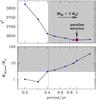 |
Fig. 2 Constraints from the xallarap fit as a function of the orbital period P of the source star. The top panel shows χ2 of the xallarap fit as a function of P, with a red circle marking the location of the best parallax model. The bottom panel shows the minimum mass of the source companion as a function of P. The shaded area in both panels indicates where models are excluded based on conservative blending constraints on the source companion’s mass. |
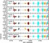 |
Fig. 3 Residual of data, with 1-σ error bars, for the various models considered. |
In Fig. 2, we show χ2
of the fit plotted as a function of the orbital period of the source star. We compare
this to the χ2 statistic of the best parallax fit. We find
that xallarap models provide fits competitive with the parallax planetary models for
orbital periods P > 1 year. However, the
solutions in this range cannot meet the constraint provided by the source brightness.
Combining Eqs. (6) and (7) with Kepler’s third law,
P2 = a3/(M1 + M2)
yields (Dong et al. 2009)  (8)Rearranging
this equation for M2, and using the fact that
M2/(M1 + M2) < 1,
we can derive an lower limit for the mass of M2,
(8)Rearranging
this equation for M2, and using the fact that
M2/(M1 + M2) < 1,
we can derive an lower limit for the mass of M2,
 (9)In the lower
panel of Fig. 2, we show the minimum mass of the
source companion as a function of orbital period. The blending constraint means that the
source companion cannot be arbitrarily massive, and we use a conservative upper limit
for its mass of 3 M⊙. With this constraint, we find that
xallarap models are not competitive with parallax planetary models, and we therefore
exclude the xallarap interpretation of the light curve.
(9)In the lower
panel of Fig. 2, we show the minimum mass of the
source companion as a function of orbital period. The blending constraint means that the
source companion cannot be arbitrarily massive, and we use a conservative upper limit
for its mass of 3 M⊙. With this constraint, we find that
xallarap models are not competitive with parallax planetary models, and we therefore
exclude the xallarap interpretation of the light curve.
4.1.2. Binary source
We also attempted to model this event as a binary source - point lens (BSPL) event; indeed it has been shown that binary sources can sometimes mimic planetary signals (Gaudi 1998). For this we introduced three additional parameters: the impact parameter of the secondary source component, u0,2, and its time of closest approach, t0,2, as well the flux ratio between the source components. We note that parallax is also considered in our binary source modelling, for fair comparison to other models. We find that the best binary-source model provides a poorer fit, with χ2 = 3809, which gives Δχ2 ~ 180 compared to our best planetary model (including parallax, see model D in the following section). Residuals for this model, as well as all other models discussed in this section are shown in Fig. 3.
4.2. Best-fit models
We searched the parameter space using an MCMC algorithm as well as a grid of (d,q,α) to locate good starting points for the algorithm (see e.g. Kains et al. 2009), over the range −4 < log q < 0 and −1.0 < log d < 2. This encompasses both planetary and binary companions that might cause the central perturbation. In Fig. 4 we present the χ2 distribution in the d,q plane. We find four local solutions, all of which have a mass ratio corresponding to a planetary companion. We designate them as A, B, C and D; the degeneracy among these local solutions is rather severe, as can be seen from the residuals shown in Fig. 3.
For the identified local minima, we then further refine the lensing parameters by conducting additional modelling, considering higher-order effects of the finite source size and the Earth’s orbital motion. It is found that the higher-order effects are clearly detected with Δχ2 > 500. Best-fit parameter for each of the local minima are given in Table 2, while Fig. 5 shows the geometry of the source trajectories with respect to the caustics for all four minima. We note that the pairs of solutions A and D, and B and C, are degenerate under the well-known d ↔ d-1 degeneracy (Griest & Safizadeh 1998; Dominik 1999); this is caused by the symmetry of the lens mapping between binaries with d and d-1. Comparing the pairs of solutions, we find that the A-D pair is favoured, with Δχ2 > 40 compared to the B-C pair. On the other hand, the degeneracy between the A and D solutions is very severe, with only Δχ2 ~ 7. In Fig. 6, we also show parameter-parameter correlations plots for model D, showing also the uncertainties in the measured lensing parameters.
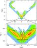 |
Fig. 4 χ2 map in the d,q plane, showing the location of the four local minima identified by our modelling runs. Out of these, local minima A and D are competitive, with local minima B and C having Δχ2 ~ 50 and 70 respectively, for the same number of parameters. Minima A and D correspond to the close and wide ESBL + parallax models discussed in the text. Different colours correspond to Δχ2 < 25 (red), 100 (yellow), 225 (green), and 400 (blue); we note that the χ2 map is based on the original data, before error-bar normalisation, and therefore the Δχ2 levels are slightly different from those given in Table 2. The top panel shows the breadth of our parameter space exploration, encompassing planetary and non-planteray mass-ratio regimes, while the bottom panel shows a zoom on the region where our local minima are located. |
Best-fit model parameters and 1-σ error bars for the four identified best binary-lens models including the effects of the orbital motion of the Earth (parallax).
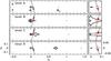 |
Fig. 5 Source trajectory geometry with respect to the caustics for all four local minima identified in Fig. 4; the source size is marked as a red circle. |
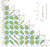 |
Fig. 6 Parameter-parameter correlations for our 9 fitted parameters. Colours indicate the limits of the 1, 2, 3, 4 and 5-σ confidence limits for each pairwise distribution. A closer view of the correlation between parallax parameters is shown on the top right inset. |
5. Lens properties
In this section we determine the properties of the lens system, using our best-fit model parameters, i.e. our wide-configuration ESBL + parallax model. We also calculated the lens properties for the competitive close-configuration model, with both sets of parameter values listed in Table 3.
5.1. Source star and Einstein radius
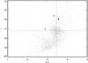 |
Fig. 7 V − I,I colour–magnitude diagram of the OGLE-2011-BLG-0251 field obtained using OGLE-IV photometry. The location of the total source + blend is indicated by a green asterisk, while the location of the deblended source is marked by a blue filled circle, and that of the blend by a red cross. The dashed lines cross at the location of the Red Clump. |
We determined the Einstein radius by first calculating the angular size of the source.
This can be done by using the magnitude and colour of the source (e.g. Yoo et al. 2004), and empirical relations between these
quantities and the angular source size. We start by using the location of the red giant
clump (hereafter RC) on our colour–magnitude diagram (Fig. 7) to estimate the reddening and extinction along the line of sight. We use an
I-band absolute magnitude for the RC of
MI,RC,0 = −0.12 ± 0.09
(Nataf et al. 2012), as well as a colour
(V − I)RC,0 = 1.06 ± 0.12
(Bensby et al. 2011). We compare these values to
those on our colour–magnitude diagram (CMD), which we generated using OGLE
I- and V-band photometry. From Fig. 7, the location of the RC on our CMD is
 (10)so, using a
distance modulus of μ = 14.52 ± 0.09, i.e. a distance to the Galactic
bulge of 8.0 ± 0.3 kpc (Yelda et al. 2011), we find
AI = 2.79 ± 0.10 and
E(V − I) = 2.39 ± 0.13.
(10)so, using a
distance modulus of μ = 14.52 ± 0.09, i.e. a distance to the Galactic
bulge of 8.0 ± 0.3 kpc (Yelda et al. 2011), we find
AI = 2.79 ± 0.10 and
E(V − I) = 2.39 ± 0.13.
Using these values, the best-fit value for the magnitude of the source IS = 15.97 ± 0.01, a source colour (V − I)S,0 = 1.15, and the empirical relations of Kervella & Fouqué (2008), we find an angular source radius θ ∗ = 10.41 ± 1.18 μas, or a source star radius of R ∗ = 10.53 ± 1.19 R⊙. This, together with the best-fit value of the source size parameter ρ ∗ , allows us to calculate the size of the Einstein radius, θE = θ ∗ /ρ ∗ . Using the relevant parameter values, we find θE = 0.749 ± 0.283 mas. This in turn allows us to calculate the source-lens relative proper motion, μrel = θE/tE = 4.28 ± 1.62 mas/yr.
5.2. Masses of the lens components
Combining Eq. (1) and Eq. (5) allows us to derive an expression for the
mass as a function of the parallax vector magnitude πE
(defined by Eq. (4)):  (11)Using values found in the
previous section, and our best-fit parallax parameter value
πE = 0.35 ± 0.05 yields a total lens mass
ML = 0.26 ± 0.10 M⊙. Using
the best-fit mass ratio parameter value of
q = (1.92 ± 0.12) × 10-3 yields component masses of
0.26 ± 0.11 M⊙ and
0.53 ± 0.21 MJ, where MJ is
the mass of Jupiter.
(11)Using values found in the
previous section, and our best-fit parallax parameter value
πE = 0.35 ± 0.05 yields a total lens mass
ML = 0.26 ± 0.10 M⊙. Using
the best-fit mass ratio parameter value of
q = (1.92 ± 0.12) × 10-3 yields component masses of
0.26 ± 0.11 M⊙ and
0.53 ± 0.21 MJ, where MJ is
the mass of Jupiter.
5.3. Distance to the lens
We can also rearrange Eq. (1) to derive an
expression for the distance to the lens DL, ![Mathematical equation: \begin{equation} \label{eq:dl} \dl=\left[\frac{1}{\ds} + \frac{\thetae^2c^2}{4GM}\right]^{-1}\cdot \end{equation}](/articles/aa/full_html/2013/04/aa20626-12/aa20626-12-eq145.png) (12)Using our parameter
values as well as the lens mass derived thanks to our parallax measurement, we find a
distance to the lens of DL = 2.57 ± 0.61 kpc. This distance
allows us to carry out a sanity check of the lens mass we derived in the previous section.
By assuming that the contribution from the blended light comes from the lens, we can
derive an upper limit to the I-band lens magnitude
MI using our best-fit blending parameter:
(12)Using our parameter
values as well as the lens mass derived thanks to our parallax measurement, we find a
distance to the lens of DL = 2.57 ± 0.61 kpc. This distance
allows us to carry out a sanity check of the lens mass we derived in the previous section.
By assuming that the contribution from the blended light comes from the lens, we can
derive an upper limit to the I-band lens magnitude
MI using our best-fit blending parameter:
 (13)where
mI,b is the apparent
I-band magnitude of the blend,
AI,L is the extinction between the observer
and the lens, and DL is in kpc. In practice,
AI,L ≤ AI
since the lens is in front of the source, so we use the extreme scenario where
AI,L = AI
to derive an upper brightness limit (lower limit on the magnitude) for the lens. We find
this to be MI,L = 2.19 ± 0.53 mag, which
corresponds to a maximum mass of the lens of
ML,max = 1.65 ±
0.23 M⊙, assuming a main sequence star mass-luminosity
relation, and assuming that the secondary lens component (i.e. the planet) does not
contribute to the blended light. This is much larger than the value we derived in
Sect. 5.2 for the mass of the primary lens
component, which suggests that some blending comes from stars near the source rather than
from the lens, although it is difficult to quantify this without an estimate of
AI,L.
(13)where
mI,b is the apparent
I-band magnitude of the blend,
AI,L is the extinction between the observer
and the lens, and DL is in kpc. In practice,
AI,L ≤ AI
since the lens is in front of the source, so we use the extreme scenario where
AI,L = AI
to derive an upper brightness limit (lower limit on the magnitude) for the lens. We find
this to be MI,L = 2.19 ± 0.53 mag, which
corresponds to a maximum mass of the lens of
ML,max = 1.65 ±
0.23 M⊙, assuming a main sequence star mass-luminosity
relation, and assuming that the secondary lens component (i.e. the planet) does not
contribute to the blended light. This is much larger than the value we derived in
Sect. 5.2 for the mass of the primary lens
component, which suggests that some blending comes from stars near the source rather than
from the lens, although it is difficult to quantify this without an estimate of
AI,L.
Finally, we can also use the distance to the lens and the size of the Einstein ring radius to calculate the projected separation r⊥ between the lens components in AU. Using our best-fit projected angular separation d = 1.408 ± 0.019, we find a projected (i.e. minimum) orbital radius r⊥ = 2.72 ± 0.75 AU.
We can compare this to an estimate of the location of the “snow line”, which is the location at which water sublimated in the midplane of the protoplanetary disk, i.e. the distance at which the midplane had a temperature of Tmid = 170 K (although other studies have noted that this temperature varies; see e.g. Podolak & Zucker 2004). The core accretion model of planet formation predicts that giant planets form much more easily beyond the snow line, thanks to easier condensation of icy material and therefore easier formation of large solid cores in the early stages of the circumstellar disk’s evolution. Kennedy & Kenyon (2008) modelled the evolution of the snow line’s location, taking into account heating of the disk via accretion, as well as the influence of pre-main sequence stellar evolution. Using a rough extrapolation of their results, we estimate that the snow line (at t = 1 Myr) for the planetary host star in OGLE-2011-BLG-0251 is located at around ~1−1.5 AU. We therefore conclude that OGLE-2011-BLG-0251Lb is a giant planet located beyond the snow line, with both of our competitive best-fit models yielding projected orbital radii larger than 1.5 AU.
We list all the lens properties in Table 3, both for the best-fit model parameters that we have used above, and for the close-configuration model, for comparison. Lens properties derived using the close-configuration model are very similar to those we found using the wide-configuration model, the only major difference being in the orbital radius. For the close model, we find an orbital radius of 1.50 ± 0.50 AU, which is close to the location of the snow line.
6. Conclusions
Our coverage and analysis of OGLE-2011-BLG-0251 has allowed us to locate and constrain a best-fit binary-lens model corresponding to an M star being orbited by a giant planet. This was possible through a broad exploration of the parameters both in real time, thanks to the recent developments in microlensing modelling algorithms, and after the source had returned to its baseline magnitude. Various second-order effects, as well as other possible, non-planetary, interpretations for the anomaly were considered during the modelling process. Based on the best-fit solution, we were able to constrain the masses and separation of the lens components, as well as various other characteristics, thanks to a strong detection of parallax effects due to the Earth’s orbit around the Sun, in conjunction with the detection of finite source size effects. We found a planet of mass 0.53 ± 0.21 MJ orbiting a lens of 0.26 ± 0.11 M⊙ at a projected radius r⊥ = 2.72 ± 0.75 AU; the whole system is located at a distance of 2.57 ± 0.61 kpc. Our competitive second-best model leads to similar properties, but a smaller projected orbital radius r⊥ = 1.50 ± 0.50. The two best-fit models are competitive and therefore we cannot make a strong claim about which orbital radius is favoured. However, comparing both values of the projected orbital radius to the approximate location of the snow line for a typical star of the mass of the primary lens component, we conclude that OGLE-2011-BLG-0251Lb is a giant planet located around or beyond the snow line. This is in line with predictions from the core accretion model of planet formation, from which we expect large planets to be more numerous beyond the snow line; this is also where microlensing detection sensitivity is at its highest, enabling us to probe a region of planetary parameter space that is difficult to reach for other methods.
Acknowledgments
N.K. acknowledges an ESO Fellowship. The research leading to these results has received funding from the European Community’s Seventh Framework Programme (/FP7/2007-2013/) under grant agreements No 229517 and 268421. The OGLE project has received funding from the European Research Council under the European Community’s Seventh Framework Programme (FP7/2007-2013) / ERC grant agreement No. 246678 to AU. K.A., D.B., M.D., K.H., M.H., S.I., C.L., R.S., Y.T. are supported by NPRP grant NPRP-09-476-1-78 from the Qatar National Research Fund (a member of Qatar Foundation). Work by C. Han was supported by Creative Research Initiative Program (2009-0081561) of National Research Foundation of Korea. This work is based in part on data collected by MiNDSTEp with the Danish 1.54 m telescope at the ESO La Silla Observatory. The Danish 1.54 m telescope is operated based on a grant from the Danish Natural Science Foundation (FNU). The MiNDSTEp monitoring campaign is powered by ARTEMiS (Automated Terrestrial Exoplanet Microlensing Search; Dominik et al. 2008). M.H. acknowledges support by the German Research Foundation (DFG). D.R. (boursier FRIA), O.W. (aspirant FRS – FNRS) and J. Surdej acknowledge support from the Communauté française de Belgique – Actions de recherche concertées – Académie universitaire Wallonie-Europe. T.C.H. gratefully acknowledges financial support from the Korea Research Council for Fundamental Science and Technology (KRCF) through the Young Research Scientist Fellowship Program. T.C.H. and C.U.L. acknowledge financial support from KASI (Korea Astronomy and Space Science Institute) grant number 2012-1-410-02. Work by J. C. Yee is supported by a National Science Foundation Graduate Research Fellowship under Grant No. 2009068160. A. Gould and B. S. Gaudi acknowledge support from NSF AST-1103471. B. S. Gaudi, A. Gould, and R. W. Pogge acknowledge support from NASA grant NNX12AB99G. The MOA experiment was supported by grants JSPS22403003 and JSPS23340064. T.S. was supported by the grant JSPS23340044. Y. Muraki acknowledges support from JSPS grants JSPS23540339 and JSPS19340058.
References
- An, J. H., Albrow, M. D., Beaulieu, J.-P., et al. 2002, ApJ, 572, 521 [NASA ADS] [CrossRef] [Google Scholar]
- Bachelet, E., Shin, I.-G., Han, C., et al. 2012, ApJ, 745, 73 [NASA ADS] [CrossRef] [Google Scholar]
- Beaulieu, J.-P., Bennette, D. P., Fouqué, P., et al. 2006, Nature, 439, 437 [NASA ADS] [CrossRef] [PubMed] [Google Scholar]
- Bennett, D. P. 2010, ApJ, 716, 1408 [NASA ADS] [CrossRef] [Google Scholar]
- Bensby, T., Adén, D., Meléndez, J., et al. 2011, A&A, 533, A134 [NASA ADS] [CrossRef] [EDP Sciences] [Google Scholar]
- Bozza, V., Dominik, M., Rattenbury, N. J., et al. 2012, MNRAS, 424, 902 [NASA ADS] [CrossRef] [Google Scholar]
- Bramich, D. M. 2008, MNRAS, 386, L77 [Google Scholar]
- Bramich, D. M., Horne, K., Albrow, M. D., et al. 2013, MNRAS, 428, 2275 [NASA ADS] [CrossRef] [Google Scholar]
- Cassan, A. 2008, A&A, 491, 587 [NASA ADS] [CrossRef] [EDP Sciences] [Google Scholar]
- Cassan, A., Kubas, D., Beaulieu, J.-P., et al. 2012, Nature, 481, 167 [NASA ADS] [CrossRef] [Google Scholar]
- Claret, A. 2000, A&A, 363, 1081 [NASA ADS] [Google Scholar]
- Dominik, M. 1998, A&A, 329, 361 [NASA ADS] [Google Scholar]
- Dominik, M. 1999, A&A, 341, 943 [NASA ADS] [Google Scholar]
- Dominik, M., Horne, K., Allan, A., et al. 2008, Astron. Nachr., 329, 248 [NASA ADS] [CrossRef] [Google Scholar]
- Dong, S., Gould, A., Udalski, A., et al. 2009, ApJ, 695, 970 [NASA ADS] [CrossRef] [Google Scholar]
- Einstein, A. 1936, Science, 84, 506 [NASA ADS] [CrossRef] [PubMed] [Google Scholar]
- Gaudi, B. S. 1998, ApJ, 506, 533 [NASA ADS] [CrossRef] [Google Scholar]
- Gaudi, B. S., Bennett, D. P., Udalski, A., et al. 2008, Science, 319, 927 [NASA ADS] [CrossRef] [PubMed] [Google Scholar]
- Gould, A. 2004, ApJ, 606, 319 [NASA ADS] [CrossRef] [Google Scholar]
- Gould, A., Dong, S., Gaudi, B. S., et al. 2010, ApJ, 720, 1073 [NASA ADS] [CrossRef] [Google Scholar]
- Griest, K., & Hu, W. 1992, ApJ, 397, 362 [NASA ADS] [CrossRef] [Google Scholar]
- Griest, K., & Safizadeh, N. 1998, ApJ, 500, 37 [NASA ADS] [CrossRef] [Google Scholar]
- Kains, N., Browne, P., Horne, K., Hundertmark, M., & Cassan, A. 2012, MNRAS, 426, 2228 [NASA ADS] [CrossRef] [Google Scholar]
- Kains, N., Cassan, A., Horne, K., et al. 2009, MNRAS, 395, 787 [NASA ADS] [CrossRef] [Google Scholar]
- Kennedy, G. M., & Kenyon, S. J. 2008, ApJ, 673, 502 [NASA ADS] [CrossRef] [Google Scholar]
- Kervella, P., & Fouqué, P. 2008, A&A, 491, 855 [NASA ADS] [CrossRef] [EDP Sciences] [Google Scholar]
- Lupton, R. 1993, J. British. Astron. Associat., 103, 320 [Google Scholar]
- Muraki, Y., Han, C., Bennett, D. P., et al. 2011, ApJ, 741, 22 [NASA ADS] [CrossRef] [Google Scholar]
- Nataf, D. M., Gould, A., Fouqué, P., et al. 2012 [arXiv:1208.1263] [Google Scholar]
- Podolak, M., & Zucker, S. 2004, Meteorit. Planet. Sci., 39, 1859 [NASA ADS] [CrossRef] [Google Scholar]
- Ryu, Y.-H., Han, C., Hwang, K.-H., et al. 2010, ApJ, 723, 81 [NASA ADS] [CrossRef] [Google Scholar]
- Sumi, T., Kamiya, K., Bennett, D. P., et al. 2011, Nature, 473, 349 [NASA ADS] [CrossRef] [PubMed] [Google Scholar]
- Udalski, A. 2003, Acta Astron., 53, 291 [NASA ADS] [Google Scholar]
- Yelda, S., Ghez, A. M., Lu, J. R., et al. 2011, in The Galactic Center: a Window to the Nuclear Environment of Disk Galaxies, eds. M. R. Morris, Q. D. Wang, & F. Yuan, ASP Conf. Ser., 439, 167 [Google Scholar]
- Yoo, J., DePoy, D. L., Gal-Yam, A., et al. 2004, ApJ, 603, 139 [Google Scholar]
All Tables
Data sets for OGLE-2011-BLG-0251, with the number of data points for each telescope/filter combination.
Best-fit model parameters and 1-σ error bars for the four identified best binary-lens models including the effects of the orbital motion of the Earth (parallax).
All Figures
|
Fig. 1 Light curve of OGLE-2011-BLG-0251. Data points are plotted with 1-σ error bars, and the upper panel shows a zoom around the perturbation region near the peak |
| In the text | |
|
Fig. 2 Constraints from the xallarap fit as a function of the orbital period P of the source star. The top panel shows χ2 of the xallarap fit as a function of P, with a red circle marking the location of the best parallax model. The bottom panel shows the minimum mass of the source companion as a function of P. The shaded area in both panels indicates where models are excluded based on conservative blending constraints on the source companion’s mass. |
| In the text | |
|
Fig. 3 Residual of data, with 1-σ error bars, for the various models considered. |
| In the text | |
|
Fig. 4 χ2 map in the d,q plane, showing the location of the four local minima identified by our modelling runs. Out of these, local minima A and D are competitive, with local minima B and C having Δχ2 ~ 50 and 70 respectively, for the same number of parameters. Minima A and D correspond to the close and wide ESBL + parallax models discussed in the text. Different colours correspond to Δχ2 < 25 (red), 100 (yellow), 225 (green), and 400 (blue); we note that the χ2 map is based on the original data, before error-bar normalisation, and therefore the Δχ2 levels are slightly different from those given in Table 2. The top panel shows the breadth of our parameter space exploration, encompassing planetary and non-planteray mass-ratio regimes, while the bottom panel shows a zoom on the region where our local minima are located. |
| In the text | |
|
Fig. 5 Source trajectory geometry with respect to the caustics for all four local minima identified in Fig. 4; the source size is marked as a red circle. |
| In the text | |
|
Fig. 6 Parameter-parameter correlations for our 9 fitted parameters. Colours indicate the limits of the 1, 2, 3, 4 and 5-σ confidence limits for each pairwise distribution. A closer view of the correlation between parallax parameters is shown on the top right inset. |
| In the text | |
|
Fig. 7 V − I,I colour–magnitude diagram of the OGLE-2011-BLG-0251 field obtained using OGLE-IV photometry. The location of the total source + blend is indicated by a green asterisk, while the location of the deblended source is marked by a blue filled circle, and that of the blend by a red cross. The dashed lines cross at the location of the Red Clump. |
| In the text | |
Current usage metrics show cumulative count of Article Views (full-text article views including HTML views, PDF and ePub downloads, according to the available data) and Abstracts Views on Vision4Press platform.
Data correspond to usage on the plateform after 2015. The current usage metrics is available 48-96 hours after online publication and is updated daily on week days.
Initial download of the metrics may take a while.