| Issue |
A&A
Volume 552, April 2013
|
|
|---|---|---|
| Article Number | A144 | |
| Number of page(s) | 11 | |
| Section | Extragalactic astronomy | |
| DOI | https://doi.org/10.1051/0004-6361/201219327 | |
| Published online | 18 April 2013 | |
Structure of the Large Magellanic Cloud from near infrared magnitudes of red clump stars
Indian Institute of Astrophysics, Koramangala II Block, 560034 Bangalore, India
e-mail: This email address is being protected from spambots. You need JavaScript enabled to view it.
; This email address is being protected from spambots. You need JavaScript enabled to view it.
Received: 2 April 2012
Accepted: 30 January 2013
Abstract
Context. The structural parameters of the disk of the Large Magellanic Cloud (LMC) are estimated.
Aims. We used the JH photometric data of red clump (RC) stars from the Magellanic Cloud Point Source Catalog (MCPSC) obtained from the InfraRed Survey Facility (IRSF) to estimate the structural parameters of the LMC disk, such as the inclination, i, and the position angle of the line of nodes (PAlon), φ.
Methods. The observed LMC region is divided into several sub-regions, and stars in each region are cross-identified with the optically identified RC stars to obtain the near infrared magnitudes. The peak values of H magnitude and (J − H) colour of the observed RC distribution are obtained by fitting a profile to the distributions and by taking the average value of magnitude and colour of the RC stars in the bin with largest number. Then the dereddened peak H0 magnitude of the RC stars in each sub-region is obtained from the peak values of H magnitude and (J − H) colour of the observed RC distribution. The right ascension (RA), declination (Dec), and relative distance from the centre of each sub-region are converted into x,y, and z Cartesian coordinates. A weighted least square plane fitting method is applied to this x,y,z data to estimate the structural parameters of the LMC disk.
Results. An intrinsic (J − H)0 colour of 0.40 ± 0.03 mag in the Simultaneous three-colour InfraRed Imager for Unbiased Survey (SIRIUS) IRSF filter system is estimated for the RC stars in the LMC and a reddening map based on (J − H) colour of the RC stars is presented. When the peaks of the RC distribution were identified by averaging, an inclination of 25°.7 ± 1°.6 and a PAlon = 141°.5 ± 4°.5 were obtained. We estimate a distance modulus, μ = 18.47 ± 0.1 mag to the LMC. Extra-planar features which are both in front and behind the fitted plane are identified. They match with the optically identified extra-planar features. The bar of the LMC is found to be part of the disk within 500 pc.
Conclusions. The estimates of the structural parameters are found to be independent of the photometric bands used for the analysis. The radial variation of the structural parameters are also studied. We find that the inner disk, within ~3°.0, is less inclined and has a larger value of PAlon when compared to the outer disk. Our estimates are compared with the literature values, and the possible reasons for the small discrepancies found are discussed.
Key words: Magellanic Clouds / galaxies: structure / stars: horizontal-branch
© ESO, 2013
1. Introduction
The Large Magellanic Cloud (LMC) is a disk galaxy with planar geometry. The orientation measurements of the LMC disk plane have been estimated previously by various authors (de Vaucouleurs & Freeman 1972; van der Marel & Cioni 2001; Olsen & Salyk 2002; and Subramanian & Subramaniam 2010) using optical data of different tracers. Reddening plays an important role in the estimation of the structural parameters of a galaxy. As the effect of reddening is less in longer wavelengths, the LMC structure estimated using near infrared (NIR) data is likely to have reduced effect due to reddening. Koerwer (2009, hereafter K09) derived an inclination, i of 23 5 ± 04, and a position angle of line of nodes, (PAlon), φ of 1546 ± 12, using the JH photometric data of red clump (RC) stars from the InfraRed Survey Facility Magellanic Cloud Point Source Catalog (IRSF MCPSC). This study, was unable to identify the warps in the southwestern end of the disk, which is evident in optical studies (Olsen & Salyk 2002; and Subramanian & Subramaniam 2010) of the structure of the LMC using the RC stars.
The sample of RC stars used in the study by K09 have contamination from stars in the other evolutionary phases, such as the asymptotic giant branch (AGB) stars. The details of the method applied for the reddening correction is not clearly mentioned in the paper by K09. The intrinsic (J − H)0 colour of the RC stars estimated by K09 is in the Johnson Cousins glass filter system. This has to be tranformed to the Simultaneous three-colour InfraRed Imager for Unbiased Survey (SIRIUS) IRSF filter system for the accurate reddening estimation. The extinction maps of the LMC estimated from the RC stars data in optical bands, which are given in the lower panels of Figs. 5 and 6 of Subramanian & Subramaniam (2010) and in Fig. 3 of Haschke et al. (2011), show variation in extinction across the galaxy. In particular, a large reddening in the southwestern disk is seen in the reddening maps where warps are identified. Hence reddening correction is an important factor in the estimation of the structural parameters and the extra-planar features of the LMC. In the analysis done by K09, there is also an overlap of sub-regions in the peripheral regions of the disk, which can cause some structural information to be averaged out. These points motivated us to re-estimate the LMC structure using the same NIR data of the RC stars used by K09. In this paper, we use the photometric data of the RC stars in the J and H pass bands from IRSF MCPSC (Kato et al. 2007). The Ks band magnitude limits of the survey is too shallow to reliably detect the RC stars.
The RC stars are core helium-burning stars, which are metal-rich and massive counterparts of the horizontal branch stars. Because they have a constant magnitude, they are standard candles for distance estimation (Stanek et al. 1998). Their constant characteristic colour makes them good tracers for reddening estimation (Subramaniam 2005b). Here we use the JH magnitudes of RC stars to understand the structure of the LMC disk. The RC stars occupy a compact region in the optical colour magnitude diagram (CMD) and are thus easily identifiable. Even though they occupy a compact region in the infrared CMD, their location is blended with the location of stars in the other evolutionary phases. In this study, we identify the RC stars in the NIR by cross-identifying with the optically identified RC stars to minimize the contamination of stars in other evolutionary phases, especially the AGB stars.
The structure of the paper is as follows. In Sect. 2 the data and the selection of the RC sample are explained. The analysis is described in Sect. 3 and the results are given in Sect. 4. The variation of structural parameters as a function of radius is described in Sect. 5. The effects of reddening and population effects of RC stars in the estimation of the structure are discussed in Sect. 6. As this work is motivated by the study of K09 and we use the same data set and tracer used in the study, we compare in Sect. 7 our results with the study of K09 in detail. The differences seen are also explained in this section. The conclusions of our study are given in Sect. 8.
2. Data
The IRSF-MCPSC (Kato et al. 2007) is an outcome of an imaging survey of the Magellanic Clouds (MCs) in the NIR bands J (1.25 μm), H (1.63 μm) and Ks (2.14 μm) from October 2001 to March 2006. The observations were made with the SIRIUS camera on the IRSF 1.4 m telescope at Sutherland, the South African Astronomical Observatory. The SIRIUS camera is equipped with three 1024 × 1024 HAWAII arrays to enable simultaneous observations in the three bands (Nagashima et al. 1999; Nagayama et al. 2003). The IRSF SIRIUS pixel scale is 0.45 arcsec/pixel, yielding a field of view of 7.7 × 7.7 arcmin2. The photometric catalogue (Kato et al. 2007) includes 14 811 185 point sources for a 40 deg2 area of the LMC and 2 769 682 sources for an 11 deg2 area of the Small Magellanic Cloud (SMC). In our present study, the LMC catalogue is used to estimate the structural parameters of the LMC using the RC stars.
We divided the IRSF MCPSC region of the LMC into 928 regions with a bin size of approximately 10.53 × 15 arcmin2. The average photometric error (magnitude range 15−20 in J and H bands) is around 0.1 mag. Photometric data with error less than 0.3 mag are considered for the analysis. A sample (J − H) vs. H CMD is shown in Fig. 1. To isolate the approximate RC location in the infrared CMD, we used the optical CMD of the corresponding sub-region. The RC stars are easily identifiable in the optical CMD as a separate component.
 |
Fig. 1 Sample NIR CMD of a sub-region in the LMC is shown. |
 |
Fig. 2 Sample optical CMD of a sub-region in the LMC. The box used to identify the RC stars is also shown. |
 |
Fig. 3 Sample NIR CMD of a sub-region in the LMC with the location of RC stars. The red points are the RC stars identified from the optical CMD of the sub-region. The box within which the RC stars in the IR CMD are distributed is also shown. |
The Magellanic Cloud Photometric Survey (MCPS; Zaritsky et al. 1997) obtained the photometry in U,B,V, and I bands of virtually all stars brighter than V = 21 mag in the MCs. The five-year survey was conducted at the Las Campanas Observatory’s 1 m Swope telescope, and the images were obtained using the Great Circle Camera (GCC, Zaritsky et al. 1996). The thinned 2048 × 2048 CCD has 0.7 arcsec/pixel scale. The survey scanned 64 deg2 of the LMC and 16 deg2 of the SMC. The IRSF observed region of the LMC comes within the MCPS observed region of the LMC. Zaritsky et al. (2004) presented the data of the LMC MCPS survey. The MCPS observed region of the LMC is also sub-divided into 1512 regions (each with an area of 10.53 × 15 arcmin2). For each sub-region, (V − I) vs. I CMD is plotted and the RC stars are identified. A sample optical CMD of the LMC is shown in Fig. 2. For all the regions, the RC stars are found to be located well within the box shown in the CMD, with boundaries 0.65 − 1.35 mag in (V − I) colour and 17.5 − 19.5 mag in I magnitude. The average photomeric error of stars in the RC magnitude range is 0.05 mag in the V and I bands. We considered only stars with error less than 0.15 mag for the identification of the RC stars.
We cross-identified the optical and infrared data and obtained the infrared (J,H) magnitudes of the RC stars identified within the box of the optical CMD (Fig. 2). Those are shown as red points in Fig. 3. Most of the RC stars are well within the box of infrared CMD, with boundaries 0.2 − 0.8 mag in (J − H) colour and 15.9 − 17.8 mag in H magnitude. Stars outside the box are not considered for the analysis. There are a few stars outside the box, especially fainter than 17.8 mag. As the H band limiting magnitude of the survey is 17.8 mag, it is justifiable to exclude those stars from the analysis. Again, from Fig. 3 we can see that the peak of the RC stars in H band is brighter than 17.8. As our method needs to identify the peak of the RC distribution, the box is used. The RC stars within the box are optically identified for all the 928 sub-regions. Only 926 out of 928 regions have reasonable numbers (100 − 3000) of RC stars to do the analysis.
3. Analysis
3.1. Identification of the peak magnitude and colour of the RC distribution
3.1.1. Method 1
The number distribution of the RC stars in H magnitude and (J − H) colour is obtained with a bin size of 0.05 mag and 0.04 mag, respectively. These distributions in colour and magnitude are fitted with a) a Gaussian function, b) a Gaussian + quadratic polynomial and c) a combination of two Gaussian functions. A non-linear least square method is used for fitting and the parameters are obtained, which are the coefficients of each term in the function used to fit the profile, the error in the estimation of each parameter and the reduced χ2 value. The errors in the parameters are calculated using the covariance matrix. By comparing the reduced χ2 values of different profile fits, we found that a combination of two Gaussian profiles, a narrow component and a broad one, fits well for the H magnitude distribution. The (J − H) colour distribution in majority of the (~60%) sub-regions fits better with a single Gaussian. The colour distributions in the remaining sub-regions are best fitted with a double Gaussian distribution or a Gaussian + quadratic polynomial. By comparing the reduced χ2 values, the best profile fit is used for further analysis.
 |
Fig. 4 Typical H magnitude distribution of a sub-region in the LMC. Gaussian profiles are shown as red and blue lines. The combined best-fit profile of double Gaussian is shown as a black line. The reduced χ2 value of the fit is 1.1. |
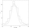 |
Fig. 5 Typical (J − H) colour distribution of a sub-region in the LMC. The best-fit profile to the distribution is also shown. The reduced χ2 value of the fit is 1.2. |
The H magnitude and (J − H) colour distributions are shown in Figs. 4 and 5 respectively. The best fit profiles are also shown in the figures. From Fig. 4 we can see that the H magnitude distribution is well represented by two Gaussian functions. Each Gaussian profile is separately shown as blue and red lines, and the combined profile is shown as a black line. The peak of the narrow component coincides with the bin with the maximum number of stars. Thus this value is taken as the RC peak magnitude for our analysis. The peak shift between the broad and narrow component ranges from 0.05 mag to 0.1 mag. The broad component peak is fainter than the narrow component peak in some sub-regions and brighter in others. The broad component may represent the thick-disk RC population and/or can be due to stars in other evolutionary phases, which are the contaminants in the sample. The NIR samples are optically selected and such a double-peak feature is not seen in optical magnitude distribution (Subramanian & Subramaniam 2010). Hence we cannot conclusively say anything about the broad component peak and dispersion. In Fig. 5, the RC colour distribution which is best fitted by a single Gaussian is shown. In 20% of the sub-regions, the RC colour distribution shows a double-peak with broad and narrow components. The peak shift between the broad and narrow components is not always in one direction. The broad component peak is bluer than the narrow component peak in some sub-regions and in others. The narrow component peak is taken as the RC peak colour. We note that the RC colour distribution in the majority of sub-regions has only one peak. The parameters that are needed to estimate the structure of the LMC are the peak H mag, peak (J − H) mag, the associated errors and the reduced χ2 values. Regions with peak errors greater than 0.1 mag and those with reduced χ2 value greater than 3.0 are omitted from the analysis. Thus the regions used for final analysis are reduced to 775 from 926. Around 85% of the sub-regions are available for the final analysis.
3.1.2. Method 2
In method 1, 15% of the sub-regions of the LMC are omitted from the final analysis due to poor fit of the RC distribution. Many sub-regions in the central region (within a radius of 2.5 degrees) are part of the omitted data points. Some of the outer regions are also omitted. The structural parameters of the LMC are very much dependent on the coverage. As a result, these inner regions, which are omitted, can make a vast difference in the estimates (Subramanian & Subramaniam 2010). The location of the bar with respect to the disk and the structural parameters of the inner region (within the radius of ~2.5−3 degrees) are some of the interesting aspects related to the structure of the LMC. Thus, to understand the structure of the LMC in more detail, it is important to increase the available regions in the inner region. Though the most appropriate method to estimate the accurate peak of the RC distribution in a sub-region is by fitting a profile by numerical analysis (method 1), we can also estimate the peak of the distribution as the average of the magnitudes of stars in the bin with largest number of stars. This allows us to estimate the peak mag of RC stars in all the sub-regions that include the central regions.
The RC stars identified are binned in both H mag and (J − H) colour with a bin size of 0.04 and 0.03 mag, respectively. The bin with largest number of RC stars is identified in both the magnitude and colour distribution. The average H mag, (J − H) colour of the stars in that particular bin and the associated standard deviation are estimated. To reduce the effect of binning in the estimation of average H mag and (J − H) colour, we identified the number of RC stars in each bin on either side of the bin with largest number of RC stars. If the number of RC stars in those bins is greater than the number ( ), where N is the largest number of RC stars identified, those stars are also included in the estimation of average values.
3.2. Estimation of E(J – H) reddening
To estimate the structural parameters of the LMC disk from the RC magnitude, we need to correct for extinction. The RC peak (J − H) mag at each location is used to estimate the E(J − H) reddening and hence the extinction in H band. The reddening is calculated using the relation  To obtain the absolute J and H band RC magnitudes and hence the (J − H)intrinsic colour of RC stars in the LMC, we used the method 1 described in Girardi & Salaris (2001). The mean RC properties as a function of time and metallicity based on Girardi et al. (2000) isochrones are available in table format at http://pleiadi.pd.astro.it. We used the star formation rate from Harris & Zaritsky (2009) and the age-metallicity relation given by Pagel & Tautvaisiene (1998) to obtain the absolute mean J and H magnitudes of RC stars in the LMC. The RC stars in the LMC have an age range. They are older than 1 Gyr and younger than 10 Gyr. We used both the 1 − 10 Gyr age range and the 1.5−9.5 Gyr one and obtained the mean magnitudes. The mean and the standard deviation of the values obtained in these two age ranges are used as the final value. The (J − H)intrinsic value is obtained as 0.47 ± 0.02 mag. K09 did a similar analysis to estimate the intrinsic colour of RC stars, assuming a constant star formation rate and a slightly different age range. The value obtained by K09 for (J − H)intrinsic is also 0.47 ± 0.06 mag, which matches with our estimate.
However, the Girardi isochrones estimate the absolute magnitudes in Bessell & Brett (1988) filters, while the IRSF SIRIUS observations are done in the MKO filter system. Thus it is important to do the necessary transformations to obtain the (J − H)intrinsic value in the MKO system. The (J − H)intrinsic value in the MKO system has to be used for the reddening correction. We did the necessary transformations (Carpenter 2001) and obtained the (J − H)intrinsic colour in the MKO system as 0.40 ± 0.03 mag. The errors in the transformation co-efficients are also considered while estimating the final error associated with the (J − H)intrinsic colour in the MKO system. In the process, the absolute mean H and J magnitudes of RC stars in the LMC are also estimated. The mean values are MJ = −1.13 ± 0.02 mag and MH = −1.53 ± 0.02 mag.
The reddening
 towards each sub-region is estimated. The interstellar extinction towards each sub-region is estimated using the relation

3.3. Estimation of the relative distance of sub-regions from the center
The dereddened H0 magnitude of the RC stars for each sub-region is estimated using H0 = H − AH. The difference in H0 mag between regions is assumed only due to their difference in the relative distance, ΔD in kpc, calculated using the distance modulus formula,
 where 50 is the distance to the center of the LMC in kpc.
3.4. Plane fitting procedure
The right ascension (RA), declination (Dec), and relative distance of a sub-region from the center are used to create a Cartesian coordinate system using the transformation equations given below (van der Marel & Cioni 2001; Subramanian & Subramaniam 2010, see also Appendix A of Weinberg & Nikolaev 2001):  where D0 is the distance to the center of the LMC, and D, the distance to each sub-region is given by D = D0 + ΔD. The (α, δ) and (α0, δ0) represents the RA and Dec of the region and the centre of the LMC, respectively. In our analysis, the optical centre of the LMC,
 (J2000) (de Vaucouleurs & Freeman 1972) is taken as the center of the LMC. According to van der Marel & Cioni (2001), the adopted center does not affect the derived parameters for the LMC disk plane (inclination, PAlon). The distance, D0 to the centre of the LMC, is taken as 50 kpc.
Once we have the x,y, and z coordinates we can apply a weighted least square plane fit to obtain the structural parameters of the LMC disk. The equation of the plane used for the plane fit is given by  From the coefficients of the plane A, B, and C, i and φ can be calculated using the formula given by.
Inclination, i = arccos( )
)  We calculated the deviations of the LMC disk from the plane with estimated coefficients. The expected z for a plane is calculated from the equation of a plane. The difference in the expected and calculated z values is taken as the deviation of the LMC disk from the plane. Thus the extra-planar features of the LMC disk are identified and quantified. Once the deviations are estimated, the regions with deviations above the error in z are omitted and the plane-fitting procedure is applied to the remaining regions to re-estimate the structural parameters of the LMC disk plane.
The uncertainty in the H and (J − H) peak values, the uncertainty in the intrinsic colour of the RC stars, and the uncertainty in the reddening law are all propagated properly to estimate the error in relative distance. The error in the z values is used in the weighted least square plane fitting procedure to obtain the error in the estimated disk parameters. Thus the error in the estimate of the LMC disk parameters is calculated by propogating the systematic errors associated with all the quantities involved in the estimation.
4. Results
4.1. NIR reddening map towards the LMC
One of the by-products of this study is the NIR reddening map towards the LMC. The shift in the peak of the (J − H) colour distribution with respect to the characteristic (J − H) colour of RC stars is a measure of reddening. The peak (J − H) colour of the RC stars in each sub-region is estimated based on methods 1 and 2. The intrinsic value of the E(J − H) colour of the RC stars in the LMC is chosen as 0.40 ± 0.03 mag. Using this value, the E(J − H) value of each sub-region is estimated as described in Sect. 3.2. A colour coded two-dimensional reddening map obtained using method 1 is shown in Fig. 6. The E(J − H) value has a range from 0.04 mag to 0.13 mag, with an average of 0.08 ± 0.03 mag. A similar plot based on method 2 is shown in Fig. 7. The E(J − H) value has a range from 0.05 mag to 0.15 mag, with an average of 0.08 ± 0.03 mag. From Figs. 6 and 7 we can see that there are slight variations in the reddening estimates when region to region is considered. However, the locations where large/less reddening is seen coincide well. Also, the range of reddening values (0.04−0.13 mag and 0.05−0.15 mag) and the average reddening (0.08 ± 0.03 mag) estimated from both the methods match well. To get a quantitative estimate of the variations, the difference in the reddening estimates obtained for each region using the two methods is calculated. The difference has a range from a minimum value of 0.0002 mag to a maximum value of 0.05 mag. In most of the regions, the difference is ≤ 0.009 mag, which is much less than the average error (0.03 mag) associated with the estimation of reddening in both the methods. Only for a few regions (less than 6%) is the difference more than 0.03. From these maps we can see that reddening varies across the LMC. The reddening is more in the southwestern regions of the LMC disk as well on the eastern side. The reddening variations here are similar to those obtained in the optical studies (Haschke et al. 2011; Subramanian & Subramaniam 2010).
 |
Fig. 6 Two-dimensional plot of reddening (E(J − H)) obtained based on method 1. |
 |
Fig. 7 Two-dimensional plot of reddening (E(J − H)) obtained based on method 2. |
 |
Fig. 8 IRSF MCPSC regions which are fitted on the plane and those which are deviated. The lower left and upper left panels are the plots which are obtained from the analysis using method 1. The lower right and upper right panels are the plots obtained from the analysis using method 2. In the lower panels, black dots represent regions on the fitted LMC plane, red dots represent regions behind the fitted plane, and blue dots represent regions in front of the fitted plane. The upper panels show only regions with deviations greater than 1.5 kpc out of the plane, and the size of the dot is proportional to the amplitude of the deviations. The blue crosses are regions in front of the plane, while the red crosses are regions behind the plane; they are identified in the optical study using MCPS data (Subramanian & Subramaniam 2010). Magenta dots are regions which are suggested as warps by Olsen & Salyk (2002). The green hexagon in both the panels represents the optical center of the LMC. |
4.2. Structural parameters of the LMC disk
4.2.1. Method 1
The structural parameters of the LMC disk are estimated using the dereddened mean H0 magnitude of the RC stars in 775 regions. This method gives an inclination of  and a PA
 for the LMC disk. The deviation of the LMC disk regions from the estimated plane are calculated as explained in Sect. 3.3. Deviations above 1.5 kpc are considered as significant deviations from the fitted plane. The lower left-hand and upper left-hand panels of Fig. 8 show the deviation of the LMC regions from the plane. From the plots we can see that there are some regions which are deviated from the planar structure of the LMC disk. Even though the coverage of MCPS is larger than that of the IRSF MCs survey and many regions have been omitted in the infrared (IR) analysis, we can see that most of the locations of deviations identified in the present study match with the locations of deviations identified from the previous optical analysis (Subramanian & Subramaniam 2010). In the southwestern LMC, there are regions which are closer to us and also farther away.
The presence of extra-planar features would affect our estimation of the structural parameters of the disk. Out of 775 regions, 91 regions show deviations greater than 1.5 kpc and are considered as real deviations. We removed these regions and re-estimated the structural parameters of the disk using the remaining 684 regions. We obtained an inclination of  and a PA
 . The dereddened RC magnitude is plotted against the axis perpendicular to the line of nodes, which is the axis of maximum gradient, it is shown in the lower panel of Fig. 9. The plot clearly shows the effect of inclination from northeast to southwest of the LMC disk. The black dots are those on the plane of the disk and the red are the extra-planar regions. The slope and y-intercept of the line fitted to the data, excluding the extra-planar regions, are 0.019 ± 0.001 mag/kpc and 16.94 ± 0.1 mag. The slope is the measure of the inclination, and the inclination estimated from the slope is 254 ± 14.
 |
Fig. 9 Dereddened RC magnitude plotted against the axis of maximum gradient. The RC magnitude estimated from method 1 and method 2 are plotted in lower and upper panels, respectively. The red points are regions which show deviation larger sigma. The direction of inclination is shown as red line. |
4.2.2. Method 2
Using this method, we obtained an inclination of  and a PA
 for the LMC disk from the analysis of 919 sub-regions. The standard deviations estimated for the peak H mag and (J − H) colour are used to approximate the error in the estimation of distance. The regions which show deviation larger than 1.5 kpc are considered as real deviation. The lower right-hand and upper right-hand panels of Fig. 8 show the deviation of the LMC regions from the plane. The optically identified deviations are also plotted. The symbols are the same as shown in the lower left-hand and upper left-hand panels of Fig. 8. Most of the deviations identified are similar to those obtained using method 1. As there are more regions in the analysis based on method 2, more extra-planar features are identified. These deviations more or less match with the optically identified deviations. The structures in the southwestern region are better revealed in this analysis. As seen earlier, in both the southwestern region along and the regions which are closer to us (which matches with the regions where warps are identified by Olsen & Salyk 2002), there are also regions which are far away from us. Based on the amplitude of the deviations in the southwestern region, the deviations closer to us are significant than those away from us. Out of 919 regions, 215 regions show deviations. These regions are removed and the structural parameters are re-estimated. An inclination of
  and a PA
 are obtained. The inclination matches well within errors with the inclination obtained based on method 1. The PAlon is slightly different. As the estimated parameters very much depend on the coverage of the data set, the variation in these values can be attributed to the greater number of inner and outer regions included in the analysis based on method 2 as compared to method 1. The dereddened H magnitude is plotted against the axis of maximum gradient and is shown in the upper panel of Fig. 9. The colour scheme is the same as that of the plot in the lower panel of Fig. 9. From the slope and intercept of the line fitted to the data points, we estimated an inclination of
  and the distance modulus to the LMC centre.
The significant result of this analysis, which is based on method 2, is that the structure of the central region is revealed. Most of the regions in the bar are on the plane, and there are only a few regions which show deviations from the plane. This suggests that the bar is co-planar with the disk. This result is very similar to the result obtained by Subramaniam & Subramanian (2009) regarding the location of the bar with respect to the disk. Even though most of the regions in the bar are on the plane of the LMC disk, there are some localized regions which are brighter than the nearby regions. There is also one region near the center which is far away from us. These suggest that the bar region of the LMC is structured.
4.3. Distance modulus
The y-intercepts obtained from the upper and lower panels of Fig. 9 are the mean H0 value of the RC stars in the LMC. The mean distance modulus to the LMC can be attained using the formula  In this equation, MH is the absolute H band magnitude of the RC stars in the LMC. MH is taken as − 1.53 ± 0.02 which is calculated in Sect. 3.2. The H0mean obtained from the lower panel of Fig. 9 (method 1) is 16.94 ± 0.1 mag and is 16.95 ± 0.1 mag from the upper panel of Fig. 9 (method 2). Then the mean distance modulus to the LMC, μ0, is 18.47 ± 0.1 mag (from method 1) and 18.48 ± 0.1 mag (from method 2). These values match with in errors with the previous estimates of 18.54 ± 0.06 mag (K09), 18.55 ± 0.01 mag and 18.5 ± 0.01 mag (from MCPS and OGLE III data sets, Subramanian & Subramaniam 2010), 18.5 ± 0.02 (Alves 2004), and 18.53 ± 0.07 (Salaris & Girardi 2002) towards the LMC.
 |
Fig. 10 IRSF MCPSC regions which are fitted on the plane and those which are deviated based on the analysis of J band data. The black dots represent regions on the fitted LMC plane, the red dots represent regions behind the fitted plane, and the blue dots represent regions in front of the fitted plane. The size of the blue and red dots is proportional to the amplitude of the deviations. |
5. Dependence of structural parameters on the photometric band
In the present study to estimate the structural parameters of the LMC disk, we assume that the variation in the extinction-corrected H band magnitude of the RC stars between various sub-regions is solely due to the distance effect induced by the structure of disk. Then the variations should be independent of the chosen photometric bands. Thus, it is useful to compare the results obtained from the magnitude distribution of RC stars in H band with that of J band analysis. The analysis in J band described below is done similarly to method 2, which is given in Sect. 3.1.2 for H band analysis. The optically identified RC stars are found to have a magnitude range of 16.4−18.4 in J band. For each of the 926 sub-regions, (J − H) vs. J CMD is plotted and the stars within the box with magnitude range 16.4−18.4 and colour range 0.2−0.8 are identified. The identified RC stars are binned in J magnitude with a bin size of 0.04 mag. The bin with the largest number of RC stars is identified in J magnitude distribution. The average J mag in that particular bin and the associated standard deviation are estimated. To reduce the effect of binning in the estimation of average J mag, we identified the number of RC stars in each bin on either side of the bin with the largest number of RC stars. If the number of RC stars in those bins is greater than the number (), where N is the largest number of RC stars identified, those stars are also included in the estimation of average values. The E(J − H) value estimated for each sub-region in Sect. 4.1 is used to find the extinction in J band for that region. The formula used (Indebetouw et al. 2005) is  The extinction-corrected J band magnitude for all the sub-regions is estimated. From the extinction-corrected J band magnitudes, the relative distance between regions and hence the z co-ordinates are obtained. A weighted least square plane fitting procedure is applied to estimate the structural parameters of the LMC disk. The deviations from the plane are also estimated. The structural parameters are re-estimated after removing the regions which show deviations larger than 1.5 kpc from the plane. An inclination of
  and a PA
 are obtained. The parameters match well within errors with the estimates from the analysis of H band data. The deviations from the plane are shown in Fig. 10. These deviations also match well with the deviations (shown in Fig. 8) obtained from the analysis of H band data. The distance modulus towards the LMC is also calculated using the J band data and is found to be 18.47 ± 0.1 mag. The results for the analysis of J band data match well with the results obtained from the analysis of H band data.
 |
Fig. 11 Variation of the structural parameters of the LMC disk as a function of radius. The upper panel shows the variation of inclination and the lower panel shows the variation of the PAlon. |
6. Radial variation of the structural parameters
In this section, the variation of the structural parameters of the LMC disk as a function of radius is studied. As the data points are found more frequently in the analysis based on method 2, we make use of that data to find the variation of the parameters as a function of the radius. We estimated the parameters using the data within different radii, starting from 1.5 degrees to 4.5 degrees with an increment of 0.1 degree. The estimates obtained are plotted in Fig. 11 as a function of radius. The lower panel shows the variation of the PAlon and the upper panel shows the variation of inclination. The parameters are more or less similar above the radius of 3 degrees. From the plot we can also see that the inner LMC (within a radius of 3 degrees) is disturbed. Inclination of the disk increases gradually from the inner to the outer region until a radius of ~3.25 degrees. The PAlon varies greatly within a radius of 2.8 degrees and then remains almost constant outwards. Variations in the inclination and position angle of line of nodes are seen within ~3-degree radius. Variations within the inner region suggest that the inner LMC, where the bar is also located, is structured/disturbed. This could be due to the the effect of tidal interactions and/or mergers experienced by the LMC. After 3.25 degrees, both parameters of the disk remain almost constant ( and PA
 ). Subramanian & Subramaniam (2010) estimated the parameters of the outer disk (regions which have a radius greater than 3°) and that of the inner disk (data within in a radius of 3 degrees). They found the inner disk to have a lower inclination and a larger PAlon and vice versa for the outer disk. As they had only a few regions in the inner 3-degree radius, they could not see the continuous trend from inner to outer region. From this analysis, we confirm that the inner structure of the LMC is different from the outer structure and that the inner disk is less inclined with a large PAlon, while the outer disk is highly inclined with less PAlon. The increase in the inclination of the outer disk, which makes the northeastern part of the LMC closer to us, could be due to the tidal interaction with our Galaxy.
Summary of orientation measurements of LMC disk plane.
7. Effect of reddening and population effects in the detection of extra-planar features
The extra-planar features identified in the disk of the LMC are important because they give clues to the interaction of the LMC with external systems. The effects of the population differences of the RC stars and reddening in the detection of the extra-planar features have to be looked at carefully to understand whether the structures identified are real or not. In this section we discuss these effects in detail.
7.1. Heterogeneous population
The RC stars in the LMC disk are a heterogeneous population and therefore have a range in mass, age, and metallicity. The density of stars in various locations will also vary with the local star-formation rate as a function of time. These factors result in a range of magnitude and colour of the net population of RC stars in any given location and would contribute to the observed peaks in magnitude and colour distributions. Therefore, the deviations found in some regions may also be due to these population differences of RC stars. But previous studies by Olsen & Salyk (2002), van der Marel & Cioni (2001), Subramaniam & Anupama (2002), Grocholski et al. (2006), and Piatti et al. (2013) suggest that the population effects in the magnitude and colour of the RC stars in the central regions of the LMC are likely to be negligible.
The contamination of the RC sample by stars in the other evolutionary phases, like the AGB stars, is less in our analysis because the stars in our sample are optically identified RC stars, as described in Sect. 2.
7.2. Effect of reddening
The extra-planar features, which are found both behind the disk and in front of the disk, could be in the plane of the LMC disk itself if there were an over-estimate or under-estimate of the reddening. It has been demonstrated by Zaritsky et al. (1997) that the extinction property of the LMC varies both spatially and as a function of stellar population. In our study, the dereddening of RC stars is done using the reddening values estimated from the RC stars themselves. In order to understand the effect of reddening, we plotted a two-dimensional plot of reddening and the deviations. The deviations and the reddening values obtained by applying method 1 and method 2 are given in Fig. 12. The lower left-hand and lower right-hand panels show the reddening distribution obtained from method 1 and method 2, respectively. The upper left-hand and upper right-hand panels show the distribution of the deviations obtained from method 1 and method 2, respectively. In the lower panels, the size of the dot is proportional to the reddening value, and in the upper panels it is proportional to the amplitude of the deviation. The red dots in the upper panels of the plots represent the regions behind the plane, while blue dots represent the regions in front of the plane. The regions in the southwestern part of the LMC disk around our suggested warps show more reddening. Thus if we assume a constant reddening across the LMC, we will not be able to identify these warps. At the same time, we do not see a strong correlation between reddening and the deviation, because both positive and negative deviations are observed for regions with large reddening, i.e., the reddening could not have been both under and over-estimated.
 |
Fig. 12 Lower left and lower right panels show the distribution of reddening across the LMC, estimated using method 1 and method 2, respectively. The size of the dots is proportional to the amplitude of the reddening. The upper left and upper right panels show the distribution of deviations from the plane estimated using method 1 and method 2 respectively. The blue dots are the regions in front of the plane, while the red dots are those behind the plane. |
8. Comparison with previous estimates
Previously, many studies were carried out to obtain the planar parameters of the LMC disk using various tracers. The values from those studies along with our estimates are summarised in Table 1. Tracers used in those studies are also mentioned in the table. From Table 1 we can see that the structural parameters have a range of values. The inclination value varies from 23° ± 0.8° to 374 ± 23 and the PAlon varies from 1225 ± 83 to 170° ± 5. Our estimates are found to be within this range. Subramanian & Subramaniam (2010) suggested that the complicated structure of the inner LMC causes variation in the estimated planar parameters, depending on the area covered for each study. In Sect. 5 we show that the inner structure of the LMC is disturbed with structural variations. Various studies of the LMC disk and bar regions (Fig. 6 given in Koerwer 2009; Fig. 2 in Subramaniam & Subramanian 2009; and Fig. 4 in Subramaniam 2003) have shown that it is a highly structured galaxy. Thus the variations in the estimate of the planar parameters are likely to be due to these structures.
8.1. Comparison with the study of K09
In our present study, we implemented the same data set and tracer used by K09 to understand the structure of the LMC disk. In this section we compare in detail the results of their study with ours. K09 obtained an inclination of 235 ± 04 and a PAlon of 1546 ± 12 for the LMC disk. Our estimates of the inclination is slightly higher than the value obtained by K09, and we estimate a lower value for the PAlon. The variation in the values of the PAlon and inclination may be due the differences in the methodologies adopted in both analyses. There is an overlap of sub-regions in the edges of the data set in the analysis of K09. In our analysis there is no overlap of sub-regions. The contamination of the RC sample by the stars in other evolutionary phases is less in our study compared to the study of K09. Also, the reddening correction adopted by K09 is not very clear. If K09 adopted a reddening correction on a star-by-star basis, the intrinsic colour chosen by K09 is for the RC stars. The reddening correction on a star-by-star basis is applicable only if all the stars in the sample are RC stars. The sample of K09 has AGB stars and also stars in other evolutionary phases. A method less susceptible to contamination is to deredden the observed peak colour corresponding to the RC stars in each sub-region. Again, from Fig. 1 of K09, which shows the location of selected sample, we can see that there are stars which have (J − H) colour less than 0.47 mag (0.47 is the intrinsic colour chosen by K09). Though we expect a spread in the colour (RC stars which are slightly bluer and slightly redder than the intrinsic colour) of the RC distribution due to population effects, internal reddening, and photometric errors, the colour selection range used by K09 is very large and includes stars from other evolutionary phases. If K09 has adopted star-by-star reddening correction, then it is not clear how they did corrections for stars bluer than 0.47 mag. The above mentioned differences could have resulted in the variation of the estimated parameters in the two studies.
 |
Fig. 13 Regions in the bar of the LMC. The size of the red and blue dots is proportional to the amplitude of the deviation. |
K09 found that the bar floats above the disk by 1 kpc and is closer to us. The bar regions are included in our analysis based on method 2. In our study, most of the bar regions are on the plane of the LMC disk. As the error associated in the estimation of the distance is ~1.4 kpc, regions which show deviations less than 1.5 kpc (1 sigma) are not considered as the real deviations in our analysis. In that case, if the bar is brighter than the disk by only 1 kpc, then it is not identified as a feature closer to us. In order to clarify this, we plotted the regions in the bar which show deviation greater than 0.5 kpc along with those which are on the plane. The plot is shown in the lower left-hand panel of Fig. 13. The upper left-hand and upper right-hand panels show regions which deviate greater than 1 kpc and 1.5 kpc respectively along with the regions on the plane. In all the panels, the blue dots are those in front of the plane, the red ones are the regions behind the plane, and the black dots are those on the plane. From the lower panel of the plot, we can see that all three types of regions are present in the bar. Among the deviated regions, there are regions which are nearer to us as well as away from us. These suggest that the bar is part of the disk and is structured. The middle and the upper panel plots also suggest the same. As mentioned in the earlier section, the differences in the methodologies adopted in our study and that of K09 may explain the difference in the results.
K09 found that major star-forming regions like 30 Dor (~at X = −1.6, Y = 0.25) and N11 (~at X = 2.27, Y = 2.52) are behind and in front of the plane, respectively. The super giant shell (given in Book et al. 2008), LMC4 (~at X = −1.1, Y = 2.45) is also found in front of the plane. To compare the locations of these deviations, we over plotted the deviations identified by K09 on the deviations identified in the present study based on method 1 and method 2 in Figs. 14 and 15 respectively. The location of 30 Dor and N11 are shown as cyan dots. In the figure we also show the location of super giant shells given by Book et al. (2008) as green dots. In the upper panel, the 30 Dor region lies on behind the plane features. In the lower panel also, the 30 Dor region lies on behind the plane feature. Thus we also find that the 30 Dor region is probably behind the disk. The star forming region, N11 also lies closer to the features located infront of the disk. The super giant shell LMC4 (~at X = −1.1, Y = 2.45) also lies nearer to us. These results match in both the studies.
 |
Fig. 14 Regions used in the analysis based on method 1 are shown. The black dots are regions on the fitted plane. The blue dots are the regions, in front of the plane, while red dots are behind the plane. The green dots are the locations of super giant shells given by Book et al. (2008). The cyan dots are the location of major star-forming regions 30 Dor and N11. The magenta lines are the approximate location of the bar. The magenta hexagon is the optical center of the LMC. |
The results of K09 did not reflect the warps identified in the southwestern regions identified by Olsen & Salyk (2002) and also by Subramanian & Subramaniam (2010) from the optical studies. Our present study identifies the warps in the southwestern region. K09 finds in this region a deviation from the plane in the opposite direction which is not very significant. In our analysis, we also find some small amplitude deviations away from the plane in the southwestern region. But along with these deviations, we find some regions which are significantly deviated from the plane so that they are closer to us. The non-identification of warps in the study of K09 may be due to two factors. One may be the lack of appropriate reddening correction by K09 for the RC stars in the southwestern region. From Figs. 6 and 7 we can see that the reddening is relatively high in the southwestern regions. A large reddening was also found in the southwestern region by Olsen & Salyk (2002). The second factor which may have contributed is the overlapping of sub-regions. In the analysis of K09 there is an overlapping of sub-regions in the southwestern end. From Fig. 8 (upper panels), we can see that both in front of and behind the plane features are present, which may get averaged out if the regions are overlapped.
9. Conclusions
The structure of the LMC disk is studied using the J and H magnitudes (NIR magnitudes) of the RC stars. We find an inclination of 266 ± 13 and a PAlon = 1483 ± 38 for the disk when the peaks were identified by profile fitting. When the peaks of the red clump distribution were identified by averaging, an inclination of 257 ± 16 and a PAlon = 1415 ± 45 were obtained. As a by-product of the study, a reddening map based on (J − H) colour of RC stars is presented.
We estimated a distance modulus, μ = 18.48 ± 0.1 mag to the LMC and the bar is found to be part of the disk, within 500 pc. The inner (r < 30) and outer (r > 3°) disk structures of the LMC are found to be different. We identified extra-planar features in the disk similar to those identified from the optical analysis of the RC stars.
 |
Fig. 15 Regions used in the analysis based on method 2. The colour coding and the symbols are the same as in Fig. 14. |
From the comparison of our results with the study of K09, who used the same data set and tracer, we found that the selection of the RC sample from optical identification helps to reduce the contamination of the sample by stars in other evolutionary phases.
Acknowledgments
The authors thank the anonymous referee for the constructive suggestions which improved the manuscript. Smitha Subramanian acknowledges the financial support provided by Council of Scientific and Industrial Research (CSIR), India through SRF grant, 09/890(0002)/2007-EMR-I. The authors also thank the IRSF team for making the data available in public.
References
- Alves, D. R. 2004, New Astron. Rev., 48, 659 [NASA ADS] [CrossRef] [Google Scholar]
- Bessell, M. S., & Brett, J. M. 1988, PASP, 100, 1134 [NASA ADS] [CrossRef] [Google Scholar]
- Caldwell, J. A. R., & Coulson, I. M. 1986, MNRAS, 218, 223 [NASA ADS] [CrossRef] [Google Scholar]
- Carpenter, J. M. 2001, AJ, 121, 2851 [NASA ADS] [CrossRef] [Google Scholar]
- de Vaucouleurs, G., & Freeman, K. C. 1973, Vistas Astron., 14, 163 [Google Scholar]
- Feitzinger, J. V., Isserstedt, J., & Schmidt-Kaler, Th. 1977, A&A, 57, 265 [Google Scholar]
- Girardi, L., & Salaris, M. 2001, MNRAS, 323, 109 [NASA ADS] [CrossRef] [Google Scholar]
- Girardi, L., Bressan, A., Bertelli, G., & Chiosi, C. 2000, A&As, 141, 371 [Google Scholar]
- Grocholski, A. J., Cole, A. A., Sarajedini, A., Geisler, D., & Smith, V. V. 2006, AJ, 132, 1630 [NASA ADS] [CrossRef] [Google Scholar]
- Harris, J., & Zaritsky, D., 2009, AJ, 138, 124 [Google Scholar]
- Haschke, R., Grebel, E. K., & Duffau, S. 2011, AJ, 141, 158 [NASA ADS] [CrossRef] [Google Scholar]
- Indebetouw, R., Mathis, J. S., Babler, B. L., et al. 2005, ApJ, 619, 931 [NASA ADS] [CrossRef] [Google Scholar]
- Kato, D., Nagashima, C., Nagayama, T., et al. 2007, PASJ, 59, 615 [NASA ADS] [Google Scholar]
- Kim, S., Staveley-Smith, L., Dopita, M. A., et al. 1998, ApJ, 503, 674 [NASA ADS] [CrossRef] [Google Scholar]
- Kim, S., Dopita, M. A., Staveley-Smith, L., & Bessell, M. 2000, IAUJD, 1, 55 [Google Scholar]
- Koerwer, J. F. 2009, AJ, 138, 1 [NASA ADS] [CrossRef] [Google Scholar]
- Luks, Th., & Rohlfs, K. 1992, A&A, 263, 41 [NASA ADS] [Google Scholar]
- Nagashima, C., Nagayama, T., Nakajima, Y., et al. 1999, Proc. Star Formation, Held in Nagoya, Japan, ed. T. Nahamoto, 397 [Google Scholar]
- Nagayama, T., Nagashima, C., Nakajima, Y., et al. 2003, SPIE, 4841, 459 [Google Scholar]
- Nikolaev, S., Drake, A. J., Keller, S. C., et al. 2004, ApJ, 601, 260 [NASA ADS] [CrossRef] [Google Scholar]
- Olsen, K. A. G., & Salyk, C. 2002, AJ, 124, 2045 [NASA ADS] [CrossRef] [Google Scholar]
- Pagel, B. E. J., & Tautvaisiene, G. 1998, MNRAS, 299, 535 [NASA ADS] [CrossRef] [Google Scholar]
- Persson, S. E., Madore, Barry, F., Krzeminiski, W., et al. 2004, AJ, 128, 223 [Google Scholar]
- Piatti, A. E., & Geisler, D. 2013, AJ, 145, 17 [NASA ADS] [CrossRef] [Google Scholar]
- Salaris, M., & Girardi, L. 2002, MNRAS, 337, 332 [NASA ADS] [CrossRef] [Google Scholar]
- Schlegel, D. J., Finkbeiner, D. P., Davis, M. 1998, ApJ, 500, 525 [NASA ADS] [CrossRef] [Google Scholar]
- Stanek, K. Z., Zaritsky, D., & Harris, J. 1998, ApJ, 500, 141 [Google Scholar]
- Subramaniam, A. 2003, ApJ, 598, L19 [NASA ADS] [CrossRef] [Google Scholar]
- Subramaniam, A. 2004, ApJ , 604, L41 [NASA ADS] [CrossRef] [Google Scholar]
- Subramaniam, A. 2005a, ApJ , 625, L47 [NASA ADS] [CrossRef] [Google Scholar]
- Subramaniam, A. 2005b, A&A, 430, 421 [NASA ADS] [CrossRef] [EDP Sciences] [Google Scholar]
- Subramaniam, A., & Anupama, G. C. 2002, A&A, 390, 449 [NASA ADS] [CrossRef] [EDP Sciences] [Google Scholar]
- Subramaniam, A., & Subramanian, S. 2009, ApJ, 703, L37 [NASA ADS] [CrossRef] [Google Scholar]
- Subramanian, S., & Subramaniam, A. 2010, A&A, 520, A24 [NASA ADS] [CrossRef] [EDP Sciences] [Google Scholar]
- van der Marel, R. P., Cioni, M. L. 2001, AJ, 122, 1807 [NASA ADS] [CrossRef] [Google Scholar]
- Weinberg, M. D., & Nikolaev, S. 2001, ApJ, 548, 712 [NASA ADS] [CrossRef] [Google Scholar]
- Zaritsky, D., Harris, J., & Thompson, I. 1997, AJ, 114, 1003 [Google Scholar]
- Zaritsky, D., Harris, J., Thompson, I. B., et al. 2004, AJ, 128, 1606 [NASA ADS] [CrossRef] [Google Scholar]
All Tables
All Figures
|
Fig. 1 Sample NIR CMD of a sub-region in the LMC is shown. |
| In the text | |
|
Fig. 2 Sample optical CMD of a sub-region in the LMC. The box used to identify the RC stars is also shown. |
| In the text | |
|
Fig. 3 Sample NIR CMD of a sub-region in the LMC with the location of RC stars. The red points are the RC stars identified from the optical CMD of the sub-region. The box within which the RC stars in the IR CMD are distributed is also shown. |
| In the text | |
|
Fig. 4 Typical H magnitude distribution of a sub-region in the LMC. Gaussian profiles are shown as red and blue lines. The combined best-fit profile of double Gaussian is shown as a black line. The reduced χ2 value of the fit is 1.1. |
| In the text | |
|
Fig. 5 Typical (J − H) colour distribution of a sub-region in the LMC. The best-fit profile to the distribution is also shown. The reduced χ2 value of the fit is 1.2. |
| In the text | |
|
Fig. 6 Two-dimensional plot of reddening (E(J − H)) obtained based on method 1. |
| In the text | |
|
Fig. 7 Two-dimensional plot of reddening (E(J − H)) obtained based on method 2. |
| In the text | |
|
Fig. 8 IRSF MCPSC regions which are fitted on the plane and those which are deviated. The lower left and upper left panels are the plots which are obtained from the analysis using method 1. The lower right and upper right panels are the plots obtained from the analysis using method 2. In the lower panels, black dots represent regions on the fitted LMC plane, red dots represent regions behind the fitted plane, and blue dots represent regions in front of the fitted plane. The upper panels show only regions with deviations greater than 1.5 kpc out of the plane, and the size of the dot is proportional to the amplitude of the deviations. The blue crosses are regions in front of the plane, while the red crosses are regions behind the plane; they are identified in the optical study using MCPS data (Subramanian & Subramaniam 2010). Magenta dots are regions which are suggested as warps by Olsen & Salyk (2002). The green hexagon in both the panels represents the optical center of the LMC. |
| In the text | |
|
Fig. 9 Dereddened RC magnitude plotted against the axis of maximum gradient. The RC magnitude estimated from method 1 and method 2 are plotted in lower and upper panels, respectively. The red points are regions which show deviation larger sigma. The direction of inclination is shown as red line. |
| In the text | |
|
Fig. 10 IRSF MCPSC regions which are fitted on the plane and those which are deviated based on the analysis of J band data. The black dots represent regions on the fitted LMC plane, the red dots represent regions behind the fitted plane, and the blue dots represent regions in front of the fitted plane. The size of the blue and red dots is proportional to the amplitude of the deviations. |
| In the text | |
|
Fig. 11 Variation of the structural parameters of the LMC disk as a function of radius. The upper panel shows the variation of inclination and the lower panel shows the variation of the PAlon. |
| In the text | |
|
Fig. 12 Lower left and lower right panels show the distribution of reddening across the LMC, estimated using method 1 and method 2, respectively. The size of the dots is proportional to the amplitude of the reddening. The upper left and upper right panels show the distribution of deviations from the plane estimated using method 1 and method 2 respectively. The blue dots are the regions in front of the plane, while the red dots are those behind the plane. |
| In the text | |
|
Fig. 13 Regions in the bar of the LMC. The size of the red and blue dots is proportional to the amplitude of the deviation. |
| In the text | |
|
Fig. 14 Regions used in the analysis based on method 1 are shown. The black dots are regions on the fitted plane. The blue dots are the regions, in front of the plane, while red dots are behind the plane. The green dots are the locations of super giant shells given by Book et al. (2008). The cyan dots are the location of major star-forming regions 30 Dor and N11. The magenta lines are the approximate location of the bar. The magenta hexagon is the optical center of the LMC. |
| In the text | |
|
Fig. 15 Regions used in the analysis based on method 2. The colour coding and the symbols are the same as in Fig. 14. |
| In the text | |
Current usage metrics show cumulative count of Article Views (full-text article views including HTML views, PDF and ePub downloads, according to the available data) and Abstracts Views on Vision4Press platform.
Data correspond to usage on the plateform after 2015. The current usage metrics is available 48-96 hours after online publication and is updated daily on week days.
Initial download of the metrics may take a while.