| Issue |
A&A
Volume 551, March 2013
|
|
|---|---|---|
| Article Number | A1 | |
| Number of page(s) | 17 | |
| Section | Stellar structure and evolution | |
| DOI | https://doi.org/10.1051/0004-6361/201219806 | |
| Published online | 07 February 2013 | |
Patterns of variability in Be/X-ray pulsars during giant outbursts
1 IESL, Foundation for Research and Technology-Hellas 71110 Heraklion Greece
e-mail: This email address is being protected from spambots. You need JavaScript enabled to view it.
2 Institute of Theoretical & Computational Physics, University of Crete, PO Box 2208, 710 03 Heraklion, Crete, Greece
3 Observatorio Astronómico de la Universidad de Valencia, 46980 Paterna, Valencia, Spain
e-mail: This email address is being protected from spambots. You need JavaScript enabled to view it.
4 European Space Astronomy Centre (ESA/ESAC), Science Operations Department, Villanueva de la Cañada, Madrid, Spain
Received: 13 June 2012
Accepted: 21 December 2012
Abstract
Context. The discovery of source states in the X-ray emission of black-hole binaries and neutron-star low-mass X-ray binaries constituted a major step forward in the understanding of the physics of accretion onto compact objects. While there are numerous studies on the correlated timing and spectral variability of these systems, very little work has been done on high-mass X-ray binaries, the third major type of X-ray binaries. Accretion-powered pulsars with Be companions represent the most numerous group of high-mass X-ray binaries. When active, they are amongst the brightest extra-solar objects in the X-ray sky and are characterised by dramatic variability in brightness on timescales of days.
Aims. The main goal of this work is to investigate whether Be accreting X-ray pulsars display source states and characterise those states through their spectral and timing properties.
Methods. We have made a systematic study of the power spectra, energy spectra and X-ray hardness-intensity diagrams of nine Be/X-ray pulsars. Energy spectra were fitted with an absorbed power-law modified by an exponential cutoff. Discrete components such as iron emission lines and cyclotron lines were represented by Gaussian and pseudo-Lorentzian profiles, respectively. Power spectra were fitted by a combination of Lorentzian functions. The evolution of the timing and spectral parameters were monitored through changes over two orders of magnitude in luminosity.
Results. We find that Be/X-ray pulsars trace two different branches in the hardness-intensity diagram: the horizontal branch corresponds to a low-intensity state of the source and it is characterised by fast colour and spectral changes and high X-ray variability. The diagonal branch is a high-intensity state that emerges when the X-ray luminosity exceeds a critical limit. The photon index anticorrelates with X-ray flux in the horizontal branch but correlates with it in the diagonal branch. The correlation between quasi-periodic oscillation frequency and X-ray flux reported in some pulsars is also observed if the peak frequency of the broad-band noise that accounts for the aperiodic variability is used. In some sources, a significant correlation between spectral and timing parameters is seen, implying and interplay between the accretion column and the inner accretion disc.
Conclusions. The two branches may reflect two different accretion modes, depending on whether the luminosity of the source is above or below a critical value. This critical luminosity is mainly determined by the magnetic field strength, hence it differs for different sources. In this work, the systems that display the two branches have critical luminosities in the range (1−4) × 1037 erg s-1.
Key words: X-rays: binaries / stars: neutron / stars: emission-line, Be / pulsars: general
© ESO, 2013
1. Introduction
The definition of source states in low-mass X-ray binaries (LMXB) and black-hole binaries (BHB) has been a very useful way to describe the rich phenomenology exhibited by these systems in the X-ray band (Hasinger & van der Klis 1989; Muno et al. 2002; Gierliński & Done 2002; Homan & Belloni 2005; van der Klis 2006; Klein-Wolt & van der Klis 2008; Körding et al. 2008; Dunn et al. 2010; Belloni 2010). A state is defined by the appearance of a spectral (e.g., power-law, blackbody) or variability component (e.g., Lorentzian) associated with a particular and well-defined position of the source in the colour–colour (CD) or hardness-intensity (HID) diagram. The physical interpretation of these components (i.e., thermal and non-thermal Comptonisation, emission from an accretion disc, quasi-periodic oscillations, etc.) allows the formulation of theoretical models and their confrontation with the observations. Different theoretical models differ in the details of the physical location and combination of these components.
As the amount of data provided by X-ray space missions increased, so did the complexity of the observed phenomenology. Although the real picture can be quite complex, two are the basic states found in neutron-star and black-hole binaries: a low-intensity, spectrally-hard state and a high-intensity, spectrally-soft state. The current understanding is that the two states reflect the relative contribution of the accretion disc on the X-ray emission (Done et al. 2007; Lin et al. 2007). When the disc emission dominates, the soft state is seen. Matter in the disc moves in near-Keplerian orbits. The innermost stable orbit of an accretion disc around a non-rotating black hole is ~3 RSchw or ~100 km for a 10 M⊙ black hole, which is of the same order of magnitude as the magnetosphere of a weakly magnetized (B ≲ 109 G) neutron star. Therefore, the accretion flows around a low-magnetic neutron star and a stellar-mass black hole in an X-ray binary are expected to be very similar (van der Klis 1994).
On the other hand, the accretion flow around a strongly magnetized (B ~ 1012 G) neutron star may be very different because in this case the magnetic field begins to dominate the dynamics of the accreting flow at much larger distance (r ≫ RSchw) and the details of how the magnetic field affects the accretion flow are not fully understood (Becker & Wolff 2007). High magnetic field neutron stars are found in binary systems orbiting a massive (spectral type late O or early B) companion.
While there have been numerous studies on the characterisation of source states in terms of timing and spectral parameters in LMXBs (van der Klis 2006, and references therein) and BHBs (Belloni 2010, and references therein), very little work of this kind has been done on high-mass X-ray binaries (HMXB), despite the fact that they represent a significant fraction of the galactic X-ray binary population. Although the discovery of rapid aperiodic variability (flickering) in the Be X-ray pulsar V0332+53 dates back to EXOSAT times (Stella et al. 1985), timing analysis on accreting pulsars have concentrated on the properties and variability of the coherent X-ray emission (pulsations) and the detection of quasi-periodic oscillations (James et al. 2010, and references therein). In contrast, the study of the aperiodic variability and broad-band noise components is very scarce (Belloni & Hasinger 1990a; Revnivtsev et al. 2009).
Massive X-ray binaries are classified according to the luminosity class of the optical component into Be/X-ray binaries (BeXB), in which the optical companion is a dwarf or subgiant star, and supergiant (luminosity class I–II) X-ray binaries. The former tend to be transient systems while the latter are persistent sources. Be stars are non-supergiant fast-rotating, B-type and luminosity class III–V stars which at some point of their lives have shown spectral lines in emission (Porter & Rivinius 2003). In the infrared, they are brighter than their non-emitting counterparts of the same spectral type. The line emission and infrared excess originate in extended circumstellar envelopes of ionized gas surrounding the equator of the B star (see Reig 2011, for a recent review).
BeXBs represent one of the most extreme case of X-ray variability in HMXBs, displaying changes in X-ray intensity that span up to four orders of magnitude. In the X-ray band, BeXBs are most of the time in a quiescence state, below the detection level of X-ray detectors. When active, the X-ray variability of BeXBs is characterised by two type of outbursts:
-
Type I outbursts are regular and (quasi)periodic events, normally peaking at or close to periastron passage of the neutron star. They are short-lived, i.e., tend to cover a relatively small fraction of the orbital period (typically 0.2–0.3 Porb). The peak X-ray luminosity during this type of outbursts is typically ≲0.2 the Eddington luminosity for a neutron star (LEdd = 1.7 × 1038 erg s-1).
-
Type II outbursts represent major increases of the X-ray flux. The luminosity at the peak of the outburst is close to the Eddington limit. These outbursts do not show any preferred orbital phase and last for a large fraction of an orbital period or even for several orbital periods. The presence of quasi-periodic oscillations and the large and steady spin-up rates measured during giant outbursts support the formation of an accretion disc during type II outbursts.
The purpose of this work is to investigate the timing and spectral variability in BeXBs that display large X-ray intensity changes (type II outbursts). Because virtually all BeXBs are pulsars, this work seeks to shed light on the X-ray phenomenology of accretion-powered pulsars.
An attempt to define source states through CD/HID and timing analysis was carried out by Reig et al. (2006, hereafter Paper I) on the hard transient X-ray pulsar V0332+53. Subsequently, this kind of analysis was extended to three other sources: EXO 2030+375, 4U 0115+63, and KS 1947+300 (Reig 2008, hereafter Paper II) in an attempt to generalise the results of Paper I. These works clearly identified the existence of two spectral branches that were called horizontal (HB) and diagonal (DB) branches according to the motion of the source in the HID. The HB is associated with low-flux and highly variable states, whereas the DB appears at high-flux states.
This paper builds up on the results of Paper II and constitutes a systematic study of the evolution of the spectral and timing variability of all the BeXB detected by RXTE that went into type II outburst in the period 1996–2011. Based on the evolution and correlations of the spectral and timing parameters and the position of the sources in the CD/HID diagrams, we aim to define and characterise source states in X-ray pulsars. The main difference with respect to Paper II, besides doubling the number of systems investigated, is the inclusion of broad-band spectral analysis and the finer sampling of the data. In Paper II, the X-ray outbursts were divided into several (between 7–9) intervals and averaged power spectra for each interval were extracted. Each interval covered typically a few days. Here, we obtain power spectra and energy spectra (PCA+HEXTE) for each pointing, which is typically few thousand seconds long. This order of magnitude increase in sampling resolution allows us to track much faster changes, likely to be associated with accretion, whereas the acquisition of energy spectra allows the search for correlations between the spectral and timing parameters.
Section 2 summarizes the observations and the characteristics of the instruments used in the analysis. Section 3 describes the methodology and techniques used in the data analysis. A detailed description of the results is given in Sect. 4. Our interpretation of the results and the implications of this work are discussed in Sect. 5. Finally, conclusions are drawn in Sect. 6.
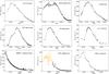 |
Fig. 1 Outburst profiles as seen by RXTE/PCA. Each point represents the average over an observation interval (typically 1000–3000 s). The count rate was obtained using the PCU2 in the energy band 4–30 keV. Different symbols denote different source states: open circles represent the diagonal branch (DB), while filled circles correspond to the horizontal branch (HB). The flaring activity during the peak of the outburst in XTE J0658–073 was analysed separately from the smoother decay. |
2. Observations
Our aim is to study the characteristics of the population of X-ray pulsars with Be companions as a whole. In order to have consistent and homogeneous data sets, we used data from one single X-ray observatory. Thanks to the All-sky Monitor (ASM) and fast reaction to unexpected events, the Rossi X-ray Timing Explorer (RXTE) has been providing large amount of data of hard X-ray transients. Its high time resolution, moderate spectral resolution and relatively broad-band response (2–150 keV) makes it the perfect observatory to undergo this type of study.
We analysed archived data obtained by all three instruments on board RXTE (Bradt et al. 1993). The data provided by the All Sky Monitor (ASM) consists of daily flux averages in the energy range 1.3–12.1 keV (Levine et al. 1996). The Proportional Counter Array (PCA) covers the energy range 2–60 keV, and consists of five identical coaligned gas-filled proportional units giving a total collecting area of 6500 cm2 and provides an energy resolution of 18% at 6 keV (Jahoda et al. 1996). The High Energy X-ray Timing Experiment (HEXTE) is constituted by 2 clusters of 4 NaI/CsI scintillation counters, with a total collecting area of 2 × 800 cm2, sensitive in the 15–250 keV band with a nominal energy resolution of 15% at 60 keV (Rothschild et al. 1998).
Due to RXTE’s low-Earth orbit, the observations consist of a number of contiguous data intervals or “pointings” (typically 0.5–1 h long) interspersed with observational gaps produced by Earth occultations of the source and passages of the satellite through the South Atlantic Anomaly. Data taken during satellite slews, passage through the South Atlantic Anomaly, Earth occultation, and high voltage breakdown were filtered out1, following the recommendations of the RXTE team2.
We have studied all BeXBs that went into outburst (the X-ray intensity increased by ≳100) during the lifetime of RXTE and have enough number of observations to allow a meaningful analysis. We did not include the BeXB candidate 4U 1901+03 because no optical counterpart is known for this source and no reliable estimate of its distance is available (Galloway et al. 2005).
Because type II outbursts are rare events, there are not many studies reporting the evolution of the spectral and/or timing parameters over the entire outburst in an accreting neutron star. An exception is 4U 0115+63, which displayed four giant outbursts during the period of time analysed in this work, in 1999, 2000, 2004, and 2008. The 2000 outburst lacks good data coverage. Here we present results for the 2004 event only. However, it is worth noticing that the source traced very similar HIDs in all outbursts. The two branches, HB and DB, are clearly distinguished in correspondence to the X-ray flux level. For an analysis of the 2008 outburst the reader is referred to Li et al. (2012) and Müller et al. (2012). The 1999 and 2004 events have also been studied by Nakajima et al. (2006) and Tsygankov et al. (2007), although these studies focus on the dependence of the cyclotron line energy with flux. Spectral and/or timing studies covering most of the same giant outbursts analysed in this work have also been performed for the following sources: V0332+53 (Tsygankov et al. 2010; Nakajima et al. 2010), KS 1947+300 (Galloway et al. 2004), EXO 2030+375 (Wilson et al. 2008), 1A 1118–616 (Nespoli & Reig 2011; Devasia et al. 2011), 1A 0535+262 (Acciari et al. 2011), XTE J0658–073 (McBride at al. 2006; Nespoli et al. 2012), GRO J1008–57 (Naik et al. 2011), Swift J1656.6–5156 (Içdem et al. 2011; Reig et al. 2011).
Figure 1 shows the outburst profiles for each source, created with the count rates of PCU2 in the 4–30 keV band. Table 1 summarises some of the properties of the systems and of the outbursts analysed in this work. Table 2 gives the proposal ID, time span, the total number of “pointings” or observation intervals, and the on-source exposure time of the observations.
Optical and X-ray information of the systems and the outbursts analysed in this work.
Journal of the RXTE observations.
3. Data reduction and analysis
In this section we describe the different techniques used in the data analysis. Heasarc FTOOLS version 6.6.3 was employed to perform data reduction, while XSPEC v12.6 (Arnaud 1996) was used for spectral analysis. Power spectra were obtained using an fast Fourier transform (FFT) algorithm implemented in a Fortran code created by us, based on subroutines from Press et al. (1996). Data reduction and model fitting were automated so that each observation was treated in exactly the same way. The same type of spectral and noise components were used for all sources. Therefore, this work constitutes the first attempt to perform a consistent, homogeneous and systematic study of the variability of accreting pulsars during giant outbursts.
3.1. Colour analysis
In analogy with optical photometry, one can quantify the broad-band X-ray spectral shape by defining X-ray colours. An X-ray colour is a hardness ratio between the photon counts in two broad bands. X-ray colours were directly obtained from the background-subtracted Standard 2 PCA light curves in the following energy bands: soft color (SC): 7–10 keV/4–7 keV and hard color (HC): 15–30 keV/10–15 keV. These ratios are expected to be insensitive to interstellar absorption effects because the hydrogen column densities to the systems, obtained from model fits to the X-ray spectra, are in the range 0.6−3 × 1022 cm-2. These values only affect significantly the X-ray spectral continuum below ~2 keV.
3.2. Spectral analysis
The spectral analysis was carried out on each individual observation using PCA (PCU2 only) Standard 2 mode data and Standard (archive) mode from the HEXTE (Cluster A generally, and Cluster B for data after December 2005, when Cluster A stopped rocking between source and background). Both instruments configurations provide a time resolution of 16s and cover their energy ranges with 129 channels. All spectra were background-subtracted and dead-time corrected. For each observation, the two spectra were fitted simultaneously, covering an overall 3–100 keV energy range. A systematic error of 0.6% was added in quadrature to the PCA spectra, slightly larger than the recommended 0.5% by the instrument team3 to obtain more conservative estimates of the spectral parameters. No systematic error was added to the HEXTE spectra because uncertainties are dominated by statistical fluctuations in this instrument. In the case of 1A 0535+262, the system which showed the most recent outburst, only PCA data were employed, covering the 3–60 keV energy range, because cluster B stopped rocking in December 2009. The model developed to obtain background counts from cluster B to be used with cluster A data is known to produce spurious line-like features around 63 keV, which for this source lies near a harmonic of a cyclotron resonant scattering feature. Also, because the signal-to-noise of the HEXTE spectra of GRO J1008–57 was very low, only PCA data were used for this source.
The lack of adequate theoretical continuum models for accreting neutron stars implies the use of empirical models to describe the observations. To compare the results from all sources consistently, we used the same (or very similar, if leading to better fit) spectral components. Table 3 gives the photon distribution for the different models. To fit the spectral continuum we used a model composed by a combination of photoelectric absorption (Balucinska-Church & McCammon 1992, PHABS in XSPEC) and a power law with high-energy exponential cutoff (CUTOFFPL). In 4U 0115+63, the CUTOFFPL model left significant residuals in the energy range 10–20 keV. For this source the POWERLAW × HIGHECUT (see White et al. 1983, and references therein) provided better fits (see Table 3 for the differences between CUTOFFPL and HIGHECUT models). For other choices of the spectral continuum the reader is referred to Kreykenbohm et al. (1999); Coburn et al. (2002); Maitra et al. (2012, and references therein). In general, the value of the hydrogen column density NH cannot be well constrained by the PCA, whose energy threshold is ~3 keV. When known from previous works with higher sensitive instruments below 3 keV, NH was fixed to the known value. To account for uncertainties in the absolute flux normalisation between PCA and HEXTE we introduced a multiplicative factor which was fixed to 1 for the PCA and let vary freely for HEXTE.
Model photon distributions used in the spectral analysis.
On top of the spectral continuum a number of discrete components are clearly present in the spectra of accreting pulsars. A Gaussian line profile (GAUSS) at 6.4 keV was used to account for Fe K fluorescence, whereas cyclotron resonant scattering features (CRSF), which we will refer to as “cyclotron lines”, were accounted for with a Lorentzian profile (CYCLABS; Tanaka 1986; Makishima et al. 1990). The width of the iron line were initially let free, but once we checked that there was no significant trend with flux, it was fixed to a value of 0.5 keV.
Pearson’s correlation coefficients for the various samples.
The sources 4U 0115+63, XTE J0658–073 and 1A 0535+262 show significant residuals around 7–10 keV. This feature is known as the “10-keV feature”, and its origin is uncertain (Coburn et al. 2002). It may appear in emission, such as in 4U 0115+63 (Ferrigno et al. 2009; Müller et al. 2012) and EXO 2030+375 (Klochkov et al. 2007) and then it is modelled with a broad Gaussian emission line, and it is referred to as the “bump” model, or in absorption, such as in XTE J0658–073 (McBride at al. 2006; Nespoli et al. 2012). In this case, a Gaussian absorption profile (GABS) is normally used4. In EXO 2030+375, this extra broad emission component is not needed if a CRSF is added at ~10 keV (Klochkov et al. 2007; Wilson et al. 2008). In 4U 0115+63, the POWERLAW × HIGHECUT model gives comparable fits to the combination of the CUTOFFPL model with a broad gaussian emission profile. Although the use of the POWERLAW × HIGHECUT model has been widely used to describe the exponential decay in the spectral continuum of many accreting pulsars, including 4U 0115+63 (Tsygankov et al. 2007; Li et al. 2012), several studies (see e.g. Kreykenbohm et al. 1999) have shown that the cutoff energy in HIGHECUT may produce an unphysical break, which may be interpreted as a line feature. Because the Ecut and the energy of the fundamental cyclotron line occupy the same region of the spectrum in 4U 0115+63, the application of the POWERLAW × HIGHECUT model to the spectrum of this source can lead to erroneous conclusions regarding the variability of the CRSF (Müller et al. 2012). In view of this, the spectral analysis of 4U 0115+63 was done using the two models.
3.3. Timing analysis
For each observation, a light curve in the energy range 2–20 keV (PCA channels 0–49) or 2–15 keV (PCA channels 0–35), depending on the data mode available, was extracted with a time resolution of 2-6 s. The light curve was then divided into 128-s segments and a FFT was computed for each segment. The final power spectrum is the average of all the power spectra obtained for each segment. The final power spectra were logarithmically rebinned in frequency and corrected for dead time effects according to the prescription given in Nowak et al. (1999). Power spectra were normalized such that the integral gives the squared rms fractional variability (Belloni & Hasinger 1990b; Miyamoto et al. 1991). To have a unified phenomenological description of the timing features within a source and across different sources, we fitted the noise components with a function consisting of one or multiple Lorentzians, each denoted as Li, where i determines the number of the component. The characteristic frequency νmax of Li was denoted as νi. This is the frequency where the component contributes most of its variance per logarithmic frequency interval and is defined as (Belloni et al. 2002) 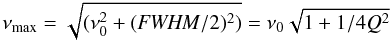 (1)where ν0 is the centroid frequency and FWHM is the Lorentzian full-width at half maximum. Note that νmax ≠ ν0. The broader the noise component, the larger the difference between νmax and ν0. The quality factor Q is defined as Q = ν0/FWHM, and is used as a measure of the coherence of the variability feature. Peaked noise is considered to be a quasi-periodic oscillation (QPO) if Q > 2.
The peaks from the neutron star pulsations were fitted to Lorentzian functions with the frequency fixed at the expected value and width equal to 0.001 Hz (approximately, the inverse of the timing resolution of the power spectra). The results from the use of Lorentzians are best visualized using the ν × Pν representation, where each power is multiplied by the corresponding frequency.
4. Results
In this section we present the results of our analysis. First, we performed an independent analysis with each one of the three techniques described above, namely, colour-intensity diagrams, energy spectra and power spectra. We searched for correlations of the colour, spectral and timing parameters as a function of X-ray flux and between various spectral parameters. Then, we investigated whether it is possible to establish relationship between parameters across different techniques. The parameters involved in these correlations are the soft (SC) and hard (HC) colours, the photon index (Γ), the cutoff energy (Ecut), the energy (EFe) and intensity (IFe) of the iron line and the characteristic frequency (νi) and fractional amplitude of variability (rmsi) of the broad-band noise components.
To quantify the strength of the relationships between different parameters we used the Pearson’s correlation coefficient r, whereas the probability p was derived to assess the significance of the correlation. p expresses the probability that the observed correlation happened by chance. The smaller the p, the more significant the relationship. If p < α, the probability that the relationship happened by chance is small. (1 − α) × 100 is the confidence level (typically 95% or 99%). p was computed from the t − value defined as 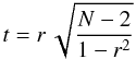 (2)where N is the number of data points. N − 2 gives the number of degrees of freedom and p = T(N − 2,t), where T is the Student’s t distribution (two-tailed).
Table 4 presents a compilation of the Pearson’s correlation coefficients and their significance for most of the samples discussed in this paper. To have an approximate perception of the quality of the fits, Cols. 7 and 8 in this table give the mean and standard deviation of the reduced χ2 values obtained from the fits to the energy and power spectra, respectively. In a few cases, most notably in 1A 0535+262, the best spectral fits gave reduced  slightly lower than 1. In those cases, however, the residuals confirmed that all the components employed by the model were necessary to describe the data. The exclusion of any of them, resulted in an overall not acceptable fit due to marked residuals that could be easily fitted with known components. For example, the removal of the cyclotron line in the higher-flux spectra of 1A 0535+262 increased the value of χ2 from 50–70 for 77 degrees of freedom to above 200 for 81 degrees of freedom. Likewise, removing the broad Gaussian component reulted in an increase of χ2 to 90–100 for 80 degrees of freedom.
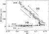 |
Fig. 2 Hardness-intensity diagram of KS 1947+300 showing two spectral branches: a low-intensity horizontal branch (HB, filled circles) and a high-intensity diagonal branch (DB, open circles). Arrows mark the flow of time. |
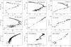 |
Fig. 3 Hardness (soft colour)-intensity diagram. The soft colour was defined as the ratio 7–10 keV / 4–7 keV. The count rate was obtained for the 4–30 keV energy band. Open circles designate points in the DB, while filled circles correspond to the HB. A logarithmic scale is used for the count rate (confront with Fig. 2). |
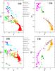 |
Fig. 4 Relationship between the X-ray colours (SC = 7–10 keV/ 4−7 keV, HC = 15–30 keV/10−15 keV) and photon index. The SC and the HC of the horizontal branch decrease as the spectrum becomes softer, as expected. In contrast, a positive correlation is seen in the HC of the diagonal branch. |
4.1. Hardness-intensity diagrams
Papers I and II showed that hard X-ray transients exhibit two distinct spectral branches in the HID that were called the horizontal branch (HB) and the diagonal branch (DB) in Paper II. As in LMXBs, these names were adopted because of the pattern that the source traces in the HID. Figure 2 shows a characteristic example of HID, that of the source KS 1947+300, where the two branches can be clearly distinguished. The average intensity in the HB is always lower than that of the DB.
The HB appears horizontal in Fig. 2 because a linear scale was used for the Y-axis. Had we used a logarithmic scale, the HB would also have a diagonal pattern, although with opposite slope (Fig. 3). In this work we shall use a logarithmic scale because it facilitates the comparison i) with other fainter accreting X-ray pulsars, as the behaviour of the points that populate the HB stands out clearer; and ii) with the HID of BHB and LMXB, as for this type of binaries a logarithmic scale is the usual way to represent the count rate. Nevertheless, for the sake of consistency with previous work, we shall keep the term horizontal branch to designate the low-intensity state and diagonal branch for the high-intensity state.
The hardness-intensity diagrams (HID) of all the sources analysed in this work, where the count rate in the 4–30 keV band is plotted as a function of the soft colour, are shown in Fig. 3. An important result that emerges from the colour analysis is that only the brightest sources display the DB (Cols. 10 and 11 in Table 1 give an estimate of the peak luminosity). However, the X-ray luminosity does not seem to be the only parameter triggering the transition between branches. KS 1947+300 and 1A 0535+262 exhibit similar peak luminosity but only KS 1947+300 displays the two branches. We shall come back to this different behaviour in Sect. 5 and show that the magnetic field strength plays a crucial role in determining the critical luminosity at which the transition takes place.
Due to their unpredictable nature, the initial stages of the rise of the outbursts lack a proper coverage. Normally, non-scheduled observations are triggered once the source is relatively bright and the reaction timescales are often similar to the time scale of the rise. Only one system, KS 1947+300, was observed for the complete duration of the outburst. In all other systems, the first data point is located, in the best cases, half way through the rise. We shall take KS 1947+300 as an example of the motion of the source in the HID. As the X-ray flux increases the SC increases, i.e., the source moves right and depicts the HB (Fig. 2, see also Fig. 3). When the luminosity reaches a critical value, the source enters the DB by making a sudden turn in the HID: it moves left and the SC starts to decrease. The peak of the outburst corresponds to the softest state of the DB. Then, as the flux decreases, the source moves back following the same track but in the opposite direction. Below the critical luminosity, the source enters the HB and the SC begins to decrease again. Arrows in Fig. 2 indicate the flow of time. In the sources that exhibit only the HB, the peak of the outburst corresponds to the hardest spectrum (largest SC).
Unlike the X-ray spectra of BHBs and LMXBs where the hard emission (i.e., above 10 keV) is well characterised by a simple power law component, the higher energy part of the X-ray spectra of BeXB is affected by extra components such as exponential cutoffs and cyclotron lines and their harmonics. As a result, the X-ray colours do not always represent a reliable measurement of the spectral slope. The HC is expected to be more affected by the distortion of the continuum because these extra components mainly appear above 10 keV. If the spectrum could be well represented by a single power law, then we would expect the X-ray colours to decrease as the emission becomes softer, that is, we would expect an anticorrelation between the photon index and the colours. The SC in both branches and the HC in the horizontal branch display this anticorrelation, albeit with large scattering in the case of the HC (Fig. 4). However, the evolution of the HC in the DB is the opposite to what it is expected, that is, the HC increases but the gamma also increases, i.e., the spectrum becomes softer. An intriguing case is V0332+53 (pink squares), whose behaviour differs from the other sources by displaying a positive correlation in three out of the four panels of Fig. 4. This peculiar behaviour of the colours of V0332+53 was already reported in Paper II. Clearly, the energy spectra of BeXBs above 10 keV are more complex than a simple power law.
4.2. Spectral variability
Although the energy spectra of all sources can be fitted with the models outlined in Sect. 3.2, the different components (power-law, cutoff, cyclotron line) fit different parts of the spectrum in different sources. Hence a direct comparison of the actual value of some of the spectral parameters (i.e., photon index) between different sources may be misleading. Nevertheless, because the spectral parameters vary smoothly along the outbursts, the search for correlations among different parameters and also with X-ray flux in each individual source is meaningful. Figure 5 shows some representative spectra for various flux levels of the HB and DB. The quoted X-ray luminosity in this figure was derived for the 2–100 keV range and normalised to the Eddington luminosity for a 1.4 M⊙ neutron star. See Table 1 for the assumed distance estimation.
The following general results are common to all or most of the sources:
-
The photon index anticorrelates with X-ray flux in the HB andcorrelates with it in the DB (Fig. 6). This means thatas the flux increases, the spectrum becomes harder in the HB andsofter in the DB. In either branch, these correlations are strong andsignificant. The Pearson’s correlation coefficient for thevariation of the photon index with flux range isρ ≪ 0.9 in most cases. Although correlations between the power-law photon index and the X-ray luminosity have been reported in the past (Reynolds et al. 1993; Devasia et al. 2011; Klochkov et al. 2011), this is the first time that a change in the slope of the correlation is seen, in correspondence with the position of the source in the HID. For 4U 0115+63, the results from the two different ways to describe the spectral continuum are plotted in Fig. 6. Circles correspond to the POWERLAW × HIGHECUT model and squares to the CUTOFFPL+GAUSS (or bump) model, where GAUSS is a broad emission Gaussian profile that accounts for the “10-keV feature” (Müller et al. 2012).
-
The cutoff energy approximately follows the same trend as the photon index, namely, it increases as the flux decreases in the HB and increases as the flux increases in the DB. As a result there is a positive correlation between the photon index and the high-energy cutoff: softer spectra correspond to high values of the cutoff energy (Fig. 7).
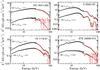
Fig. 5 Average energy spectra of the horizontal and diagonal branches at various flux levels. Black and red symbols represent PCA and HEXTE data, respectively. The quoted X-ray luminosity corresponds to the 2–100 keV range.
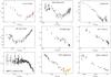
Fig. 6 Power-law photon index as a function of X-ray luminosity. Open circles represent the DB (supercritical regime), filled circles the HB (subcritical regime). Orange data points in XTE J0658–073 correspond to the flaring episode during the peak of the outburst (see Fig. 1). In 4U 0115+63, red squares represent the results from the “bump” model (see text). The Eddington luminosity for a neutron star was taken to be 1.7 × 1038 erg s-1.
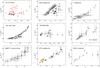
Fig. 7 Cutoff energy as a function of the photon index. Open circles represent the DB, filled circles the HB. Orange data points in XTE J0658–073 correspond to the peak of the outburst. In 4U 0115+63, red squares represent the results from the “bump” model.
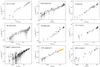
Fig. 8 Flux of the iron line as a function of the X-ray continuum flux. We assume LEdd = 1.7 × 1038 erg s-1. Open circles represent the DB and filled circles the HB.
-
The fluorescent iron Kα line feature that results from reprocessing of the hard X-ray continuum in relatively cool matter is ubiquitous in all sources. Near neutral iron generates a line centered at 6.4 keV. As the ionisation stage increases so does the energy of the line. However, the energy separation is so small that even ionised iron up to Fe XVIII can be thought as part of the 6.4 keV blend (Ebisawa et al. 1996; Liedahl 2005). The central energy of this component does not vary significantly during the outbursts and it is consistent with “near-neutral” material, that is, with the composite of lines from Fe II-Fe XVIII near 6.4 keV. The flux of the line increases with the continuum X-ray flux, indicating that as the illumination of the cool matter responsible for the line emission increases, so does the strength of the line (Fig. 8). In general, the line equivalent width remained insensitive to luminosity changes. The strong correlations of Fig. 8 imply that the contribution from thermal hot plasma located along the Galactic plane (Yamauchi et al. 2009) is not significant. We would expect the ridge emission to affect the data only for very faint observations, i.e., at the start and end of the outbursts (Ebisawa et al. 2008). The small deviation from the linear trend with flux at very low fluxes would be consistent with this statement (Fig. 8).
-
There is no universal trend between the energy of the cyclotron line and X-ray luminosity (Fig. 9). Previous studies have shown a strong anticorrelation in V0332+53 (Tsygankov et al. 2010), somehow weaker anticorrelation in 4U 0115+63 (Mihara et al. 2004; Nakajima et al. 2006) and no correlation in 1A 0535+262 (Caballero et al. 2007). We confirm the decrease of the cyclotron line energy with luminosity in V0332+53, but we do not find a smooth anticorrelation in 4U 0115+63. When the POWERLAW × HIGHECUT model is used, the energy of the cyclotron line remains fairly constant within each branch, but its value is higher in the HB (~16 keV) than in the DB (~11 keV). This result agrees with that of Tsygankov et al. (2007) and Li et al. (2012), who reported a discontinuity in the Ecyc − LX relationship of this source with larger values of the cyclotron line energy at low flux. However, if the continuum is fitted with the CUTOFFPL model and a broad emission Gaussian, then no correlation is seen, in agreement with Müller et al. (2012). In Fig. 9, red squares represent the best-fit values of the energy of the cyclotron line using the “bump” model, while circles represent those obtained with the high-energy exponential cutoff model. Our results also show no clear trend between the energy of the cyclotron line and luminosity in 1A 1118–616, EXO 2030+375, and XTE J0658–073. However, we report, for the first time, a positive correlation between the cyclotron energy and X-ray luminosity in 1A 0535+262 on long timescales (Fig. 9). A correlation had been reported only in the pulse-to-pulse analysis (Klochkov et al. 2011). Previous studies did not find any evidence for variability (Terada et al. 2006; Caballero et al. 2007). However, note that these works show observations of 1A 0535+262 when the X-ray luminosity was ≲1 × 1037 erg s-1 (LX/LEdd < 0.1). As can be seen in Fig. 9, the energy of the cyclotron line begins to increase above this value5. We verified that this relationship cannot be due to any artificial correlation between the line energy and the other parameters of the model by plotting the contours of the confidence regions of Ecyc and any other parameter. Additionally, a linear correlation analysis gives a linear correlation coefficient of 0.89 and a probability that the points are not correlated of 6 × 10⁻⁸. To ensure that the Lorentzian profile was fitting the CRSFs and not the continuum, we carefully verified that the corresponding width had reasonably narrow values. In all the cases, we obtained width values compatible with previous works. For EXO 2030+375 and 4U 0115+63, which displays the lowest energy CRSF, the obtained width is of the order of 3 keV (Wilson et al. 2008; Müller et al. 2012); for V0332+53 and 1A 0535+262, the retrieved width was of the order of 6–8 keV (Tsygankov et al. 2010; Caballero et al. 2007); 1A 1118–616 and XTE J0658–073, the systems that display the highest energy CRSF, also show the largest width, of 12–15 keV (Doroshenko et al. 2010; McBride at al. 2006).
-
The X-ray spectrum of the accreting pulsars analysed in this work is characterised by a power law (Γ = 0−1) with an exponential cutoff in the range 10–20 keV. However, the spectral continuum may be very distorted by the presence of cyclotron resonant scattering features. Unlike BHBs or anomalous X-ray pulsars where the presence of different components (disc blackbody and power law, or two power laws) causes a sudden break in the continuum, the X-ray spectral continuum of accreting pulsars does not show any evidence for an abrupt change below or above 10–20 keV (Fig. 5), despite the fact that physical models such as those by Becker & Wolff (2007) and Ferrigno et al. (2009) show that several well-defined physical components (i.e., thermal and bulk Comptonisation, blackbody emission at the base of the accretion column) are present.
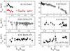 |
Fig. 9 Variation of the energy of the cyclotron line with luminosity (3–30 keV). Filled circles correspond to the HB and open circles to the DB. In 4U 0115+63, red squares represent the results from the “bump” model, whereas circles are the best-fit cyclotron energy with the POWERLAW × HIGHECUT description of the spectral continuum. |
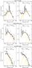 |
Fig. 10 Representative power spectra of the horizontal and diagonal branches at various flux levels for the fast-rotating pulsar 4U 0115+63 (up), EXO 2030+375 (middle) and the slow pulsator 1A 0535+262 (down). Note the shift toward higher frequencies at high flux. In 1A 0535+262, L0 is not seen at low luminosities because it lies outside of the frequency interval considered. Other features such as LLF in 4U 0115+63 or a QPO at ~40 mHz in 1A 0535+262 are shown. The Lorentzian profiles of the pulse peaks and the QPO were removed for clarity. |
4.3. Timing aperiodic variability
We conducted a systematic analysis of the rapid aperiodic variability of the sources. Our aim is to provide a consistent description of the power spectra of all sources, investigate whether the changes in spectral state are also evident in the power spectra, and study the evolution of the noise parameters throughout the outburst.
We consistently used the same model to fit the power spectra of all sources. We found that the majority of power spectra are well represented by the sum of up to three Lorentzian profiles that were termed as Li, where i = 0,1,2. Some power spectra displayed more complex substructure, which mainly consisted of the presence of wiggles without any preferred frequency range or narrow, generally weak, features confined to only one bin. Although these features may lead to a formally unacceptable fit (χ2 > 2) in some cases, no attempt to correct for this effect was carried out because it does not affect our results significantly. Here we focus on the broad-band noise components, that is, power covering relatively large frequency intervals. The use of Lorentzian profiles is particularly suitable for this kind of studies as it has been demonstrated in black-hole binaries (Pottschmidt et al. 2003; Axelsson et al. 2005). Although it cannot model very narrow features, it provides a simple but consistent way to fit the main characteristics of the power spectra across different states and to track changes occurring on short timescales. In addition to the broad-band noise represented by Li, the fast rotating pulsars 4U 0115+63 and V0332+53 show other narrower components, whose characteristic frequency does not vary with luminosity. For a more detailed analysis of these components the reader is referred to Paper II. The peaks that correspond to the spin period and its harmonics were also fitted with Lorentzian profiles but the centroid frequency and width were fixed. Figure 10 shows some representative power spectra at various flux levels.
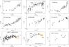 |
Fig. 11 Characteristic frequency of the main component of the broad-band noise as a function of X-ray luminosity. Open circles represent the DB (supercritical regime), filled circles the HB (subcritical regime). In XTE J0658–073, orange circles correspond to the flares. In Swift J1656.6–5156, open circles (in orange) and open squares give the frequency of L1 with and without the L2 component, respectively. We assume LEdd = 1.7 × 1038 erg s-1. |
L0 is a zero-centred Lorentzian that accounts for the noise below 0.05 Hz. L1 is the main noise component and accounts for the noise in the range 0.1–1 Hz. It is also a zero-centred Lorentzian whose characteristic frequency increases as the flux increases. Its rms is always larger than 15%. L2 accounts for the broad-band noise at higher frequencies. Its characteristic frequency peaks typically in the range 1–5 Hz, while the rms is normally below 15%. L2 appears at high flux, i.e., near the peak of the outbursts. This component is normally not statistically significant at the end of the outbursts. Although in most cases it shows up as a zero-centred Lorenztian, it may turn into peaked noise, especially at the highest flux. Because of the narrower frequency range covered by the L0 component and typically larger error bars of low-frequency points, the addition of L0, especially for the first appearance of this component, did not generally improved χ2 significantly. Hence, the addition of L0 was based on visual inspection of the residuals. In contrast, the introduction or removal of L2 was based on whether its presence or absence resulted in a significant improvement of the best fit χ2.
The following general results are common to all or most of the sources:
-
The characteristic frequency increases as the X-ray luminosityincreases (Fig. 11).
-
Whereas the overall 0.01–10 Hz rms does not change significantly within a branch, the fractional amplitude of variability of the main component (L1) tends to decrease as the X-ray luminosity increases (Fig. 12). With the exception of EXO 2030+375, this trend is more distinct for sources exhibiting two branches. That is, the source tends to be more variable in the HB.
-
L0 and L2 are usually not present in the HB. The disappearance of L0 in the HB is probably due to the fact that this component falls below the frequency interval considered (ν0 < 0.01 Hz) at very low fluxes in agreement with the observed frequency shift (Fig. 11).
-
Whenever L1 and L2 appear simultaneously in the power spectrum, their frequencies correlate (Fig. 13).
The saturation at high luminosity seen in the luminosity-frequency diagram of some sources (most notably in XTE J0658–073, Swift J1656.6–5156, and EXO 2030+375) is due to the appearance of the L2 component. The correlation between the characteristic frequency and the flux is broken when this extra component is added because it prevents L1 from shifting toward higher frequencies. As an exercise, we removed the L2 component from the power spectra of Swift J1656.6–5156. The absence of L2 gives worse fits, but ν1 shifts up (squares in Fig. 11) and the correlation holds even at the highest luminosity.
4.4. Correlation between spectral and timing parameters
The spectral parameters correlate tightly with the X-ray flux. In some sources, though, this correlation changes sign at very low fluxes (in the HB). The characteristic frequency of the broad-band noise also shows a smooth relationship with flux, albeit with more scattering. The question is then whether the spectral and timing parameters correlate with each other. Figure 14 displays the L1 maximum frequency as a function of the photon index. These two parameters seem to correlate in most sources, although the sign and strength of the correlation vary significantly. We shall discuss the implication of this result in Sect. 5.3.
5. Discussion
The main goal of this study is to perform a detailed spectral and timing analysis of accretion-powered pulsars with Be companions in an attempt to characterise this type of systems as a group. More precisely, we wish to investigate i) whether accreting X-ray pulsars display spectral states as black-hole and low-mass X-ray binaries do and characterise those states; and ii) to search for correlations between spectral and timing parameters during major outbursts in an attempt to constrain the accretion models in X-ray pulsars.
In this section we discuss the implications of our work. We interpret our results in the context of the model that suggests the existence of two different accretion regimes, defined by a critical luminosity (Becker et al. 2012). First, we make a short introduction of the spectral formation mechanism in accreting pulsars and then we summarise and discuss our results.
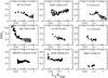 |
Fig. 12 Variation of the fractional amplitude of variability of component L1 with luminosity. Filled black circles correspond to the HB and open circles to the DB. |
5.1. Spectral formation
A detailed description of the emission properties of an accretion-powered pulsar is a complex task. First, it requires an understanding of the processes by which mass is transferred, captured, deposited on the neutron star surface in the form of an accretion column and converted into high-energy radiation. Second, this radiation has to find its way out, which involves a knowledge of the interactions of the X-rays produced close to the neutron star surface with the highly magnetized plasma forming the magnetosphere. Third, the X-rays emanating from the polar caps are subjected to absorption and reflection processes due to the ambient matter.
This complexity translates into a lack of a fundamental physical model that yields results that agree with the observations. The common practice is then to fit phenomenological multicomponent models to the energy spectra of accretion-powered pulsars. The parameters of these model components are difficult to interpret physically. Some attempts to alleviate this situation have been made by Becker & Wolff (2005, 2007, see also Ferrigno et al. 2009, who developed a new model for the spectral formation process in X-ray pulsars based on the bulk and thermal Comptonisation of photons due to collisions with the shocked gas in the accretion column. The accretion flow is channelled by the strong magnetic field into the polar caps, creating an accretion column. Most of the photons are produced at the base of the column, just above the neutron star surface (thermal mound). The low-energy (blackbody) photons created in the mound are upscattered due to collisions with electrons that are infalling at high speed (bulk Comptonisation). Thermal Comptonisation (in this case high-energy photons lose energy) also plays a significant role in shaping the spectrum and it is responsible for the formation of the exponential cutoff.
5.1.1. Two accretion regimes
There exists a critical luminosity, Lcrit, at which the deceleration of the accreting flow to rest at the neutron star surface changes from being dominated by radiation pressure to occur via Coulomb interactions (Basko & Sunyaev 1976). Becker et al. (2012) suggested that these two different regimes can explain the bimodal behaviour of the variability of the cyclotron energy with luminosity. Some sources, such as V0332+53 display a negative correlation between the cyclotron energy and the source luminosity, others, such as Her X–1 (Staubert et al. 2007), show a positive correlation.
Two accretion regimes have also been invoked by Klochkov et al. (2011) to explain the pulse-to-pulse variability in some X-ray pulsars. It is illustrative to compare our results with those of Klochkov et al. (2011) because of the different timescales involved. We have studied the long-term variability patterns of accreting pulsars by sampling timescales of X-ray variability of the order of 1000 s. Klochkov et al. (2011) studied the pulse-to-pulse spectral variability, i.e., timescales of the order of the pulse period (Pspin ~ 1−100 s). Their sample included four X-ray pulsars, three of which appear in our list: V0332+53, 4U 0115+63, and 1A 0535+262. To achieve enough photon statistics they restricted their analysis to high-flux states. In the context of the present work, this means that they analysed data of the DB in V0332+53 and 4U 0115+63 and of the high-flux part of the HB in 1A 0535+262. Despite the order of magnitude difference in the variability range, the same correlations are observed. They found that the photon index of the power-law component correlates with X-ray intensity in V0332+53 and 4U 0115+63, but anticorrelates in 1A 0535+262, which is the same result as our Fig. 6. Likewise, they reported a correlation between the energy of the fundamental cyclotron line with count rate in 1A 0535+262, as we do with our long-term pulse-average spectral analysis (Fig. 9).
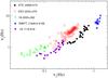 |
Fig. 13 Relationship between the peak frequencies of L1 and L2. |
5.2. Source states
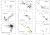 |
Fig. 14 Relationship between the characteristic frequency of the main component of the broad-band noise and the power-law photon index. In EXO 2030+375, due to the hysteresis observed in the frequency-luminosity diagram (Fig. 11) only points that correspond to the decay (after MJD 53 980) have been plotted for clarity. |
This work shows that, as BHBs and LMXBs, accreting X-ray binaries with high-mass companions also exhibit spectral states in the hardness-intensity diagrams. At low and intermediate X-ray luminosities the sources populate the HB, whereas at higher luminosities the sources trace a DB. However, unlike BHBs and LMXBs, where the hardness of the source is a distinguishing property of the accretion states (the so-called hard and soft states), the spectral branches in accretion-powered pulsars roughly sample the same colour interval. If a source displays the two branches, then the timescales of the colour and flux changes are faster in the HB than in the DB. The source covers the HB in hours to few days and the DB in days to weeks. In contrast, systems that show only the HB can remain in that branch for weeks.
With the exception of 4U 0115+63 and V0332+53 (see Paper II), there is no clear evidence for hysteresis in the HID, i.e., the same colour corresponds to two different values of the count rate depending on whether the source is in the rise or decay. This lack of hysteresis could be due to the fact that, in most cases, the rise of the outburst is much badly sampled than the decay (see Fig. 1). For Swift J1656.6–5156, 1A 0535+262, 1A 1118–616, and GRO J1008–57, no or very few data points of the rise were observed. On the other hand, in KS 1947+300, which is the source with the most complete coverage of the rise, no indication of hysteresis is found. To check this result, we performed a colour analysis on the ASM light curves and we did not find significant deviations between the rising and decaying tracks. However, it should be noticed that the errors of the ASM colours are, in the best case, roughly of the same size as the amplitude of the hysteresis effect. It is also worth mentioning that while we did not observe significant hysteresis in the HID of EXO 2030+375, the characteristic frequency of the broad-band noise in this source exhibits lower values during the rise than during the decay (Fig. 11).
One of the main findings of this work is that the transition from the HB to the DB occurs when the source luminosity increases above a certain value, which we find to be in the range ~0.06–0.3 LEdd (~1–4 × 1037 erg s-1). We observe that this value is different for different sources. We suggest that the luminosity at which the transition occurs is related to the critical luminosity and that each spectral branch can be associated with one of the two modes of accretion proposed by Becker et al. (2012). The DB, which corresponds to a high-luminosity state, would be associated with the supercritical mode and the HB with the subcritical one.
The case of KS 1947+300 and 1A 0535+262 would corroborate this association. These two sources reached similar peak outburst luminosity. However, only KS 1947+300 shows the two branches. KS 1947+300 reached a peak luminosity of 0.4 LEdd and made the transition from the HB to the DB at ~0.06 LEdd or ~1 × 1037 erg s-1, assuming a distance of ~10 kpc (Negueruela et al. 2003). In contrast, 1A 0535+262, with the same peak luminosity stayed in the HB during the entire outburst. We conclude that the intensity of the source is not the only parameter triggering the change of state and some other parameter must play a role too. The magnetic field appears as the best candidate to drive the transition. According to Becker et al. (2012), the critical luminosity Lcrit depends on the magnetic field, or equivalently, on the energy of the cyclotron line. The higher the magnetic field, the higher the critical luminosity. For typical neutron star parameters (see Becker et al. 2012, for details), the critical luminosity can be estimated as  (3)where Ecyc is the energy of the cyclotron line. 1A 0535+262 displays one of the highest energy cyclotron lines, at ~50 keV (Caballero et al. 2008). Substituting in the above equation yields Lcrit ≈ 7 × 1037 erg s-1, which is slightly larger than the outburst peak luminosity. No cyclotron line has been reported for KS 1947+300, which would indicate a lower magnetic field, in agreement with the lower luminosity at which the spectral transition occurs. The luminosity at which the transition is observed in KS 1947+300 would imply a cyclotron line at around 8 keV. Unless the cyclotron line is very strong such a feature would be difficult to detect because it would lie in a region where other spectral features dominate. First, the fluorescence iron line at 6.4 keV and possible its associated absorption edge. Second, some X-ray pulsars show significant wiggle residuals at 8–12 keV, whose origin is unclear (Coburn et al. 2002). Nevertheless, it is worth noticing that in the high-flux average spectrum of KS 1947+300, an additional absorption component at about 9 keV provides an improved fit with respect to the model used for the individual spectra. The χ2 decreases from 104 for 72 degrees of freedom to 74 for 69 degrees of freedom. This component can be modelled with an absorption Gaussian profile (GABS) and could be associated to a cyclotron line that in the single spectra would be too weak to be unveiled. The absorption could also be accounted for with an edge (χ2 = 71 for 70 degrees of freedom), although in this case the inspection of residuals reveals that this component is unable to properly fit the entire spectral region of interest. In short, it is difficult to tell whether the source actually displays a cyclotron line at this energy, but if so, its low characteristic energy would agree with the critical luminosity reached by the system.
The larger magnetic field in 1A 0535+262 might also explain the reason that previous studies of this source did not find a correlation between the energy of the cyclotron line and the X-ray luminosity. Terada et al. (2006) speculated that this energy might begin to change at a higher luminosity if the object has a higher surface magnetic field. Here we report observations of 1A 0535+262 at higher luminosities than previous studies (Kendziorra et al. 1994; Wilson et al. 2005; Caballero et al. 2007; Terada et al. 2006). As it can be seen in Fig. 9, the energy of the CRSF only begins to increase significantly when the X-ray luminosity is above ~3 × 1037 erg s-1.
XTE J0658–073 is another source whose peak luminosity is close to its critical luminosity (see Table 1). Although it does not display a proper DB, an attempt to move to that branch can be observed in Figs. 3 and 6. In particular, note the upward turn of the photon index at LX ~ 0.1 LEdd in Fig. 6.
Becker et al. (2012) also showed that as the luminosity increases, the height of the emission zone inside the accretion column approaches the neutron star surface in the subcritical accretion state, while this emission zones moves upward in the supercritical accretion state. Comptonisation occurs in the region between the radiative shock and the neutron star surface (the sinking region). In the supercritical state this region is relatively small, just a few tens of meters (see Eq. (40) in Becker et al. 2012), but its height increases as the luminosity increases. In this region, the effective velocity of the comptonising electrons is highly reduced because diffusion (outwards) and advection (inwards) are almost balanced. Hence photons would not acquire enough energy through bulk Comptonisation to populate the higher energy band and a softening of the spectrum would be expected with increasing luminosity. This agrees with the observations: in the DB, the spectrum becomes softer (soft colour decreases, Γ increases) as the luminosity increases (Figs. 3 and 6). In the subcritical mode, the typical emission height is a few kilometers (see Eq. (51) in Becker et al. 2012) but decreases as the X-ray luminosity increases. As the size of the sinking region decreases with increasing luminosity, the optical depth increases, which results in harder photons. In the HB, the spectrum becomes harder as the luminosity increases.
Finally, it is worth noticing that the four sources that display the two states have short orbital (Porb < 50 days) and spin (Pspin ≪ 100 s) periods, whereas the sources that do not transit to the DB have, in general, Porb > 100 days or Pspin ≪ 100 s (see Table 1). The result that systems harbouring fast-rotating neutron stars in narrow orbits display two branches in the HID can be linked to the work by Reig (2007), who found that BeXB with short spin and orbital periods are more variable in the X-ray band, i.e., they exhibit higher amplitude of variability as measured by the root-mean-square rms over the long-term (years) X-ray light curves. Reig (2007) explained this result in the context of the viscous decretion disc model (Okazaki & Negueruela 2001). This model predicts the truncation of the Be star’s disc due to the tidal interaction exerted by the neutron star. In the truncated disc model, the material lost from the Be star accumulates and the disc becomes denser more rapidly than around an isolated Be star (Okazaki et al. 2002). Truncation is favoured in systems with short orbital periods and low eccentricities. In such systems mass transfer would occur only when the disc is strongly disturbed. Accretion of large amount of material from the distorted disc would give rise to very bright X-ray outbursts.
5.3. Correlation of spectral and timing parameters
We searched for correlations between the different model parameters that describe the energy and power spectra. Two approaches were taken to investigate the relation between the X-ray emission and the rapid aperiodic variability. In the first one, we tracked the spectral and timing parameters following an X-ray outburst, in which case the general trend of the relation with luminosity was inferred (Figs. 6, 8, 9, 11 and 12). In the second approach, we directly compared parameters between themselves (Figs. 7 and 14). To quantify and assess the statistical significance of the various relationships we obtained the Pearson’s correlation coefficient. The results are summarised in Table 4.
Of particular interest are the correlations between spectral and timing parameters. According to the model by Becker & Wolff (2007), the hard power-law component is due to bulk inverse Comptonisation in the accretion column. Low-energy photons are upscattered in the shock and eventually diffuse through the walls of the column. Therefore, the photons that populate the hard power-law tail come from a region close to the surface of the neutron star (length scales ~106 cm).
On the other hand, aperiodic variability must be generated at much larger distance. The evidence in support of this statement comes from the correlation between the characteristic frequency of the broad-band noise and the X-ray flux and from the milliHertz range of frequencies of the QPO seen in accreting X-ray pulsars.
The radius of the magnetosphere, rm, depends on the mass accretion rate (Davies & Pringle 1981) 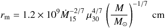 (4)where Ṁ15 is the mass accretion rate in units of 1015 g s-1 and μ30 the dipole magnetic moment in units of 1030 G cm3. As the X-ray flux increases, presumably as a consequence of an increase in the mass accretion rate, the magnetospheric radius decreases. If the processes that originate the broad-band noise are linked to motion of matter outside the magnetosphere, then we would expect that as the magnetosphere shrinks, the characteristic frequency increases, as observed (Fig. 11). Thus this correlation is consistent with and extra-magnetospheric origin of the aperiodic variability.
Likewise, QPOs in HMXB lie typically in the milliHertz range (James et al. 2010). If one assumes that QPOs are produced as a result of Keplerian motion of inhomogeneities in an accretion disc, this frequency range (0.01–1 Hz) agrees with the QPO being originated outside (but near) the magnetosphere, i.e., at length scales rm ≪ 108 cm. Indeed, a Keplerian frequency of νQPO = 100 mHz would correspond to a radius 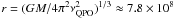 cm. Note also that in LMXBs, peaked (broad-band) noise have been seen to developed into QPOs, indicating a physical relationship between broad-band noise and QPOs (van der Klis 2006). Thus it is reasonable to assume then that the aperiodic variability originates from the same physical region as the QPOs.
Since the power-law photons and those responsible for the aperiodic variability originate in very different physical regions, we would not expect the spectral and timing parameters to correlate. We have plotted the relationship between the power-law photon index and the frequency of the main noise component L1 in Fig. 14. Despite the different location of the production mechanisms, a distinct correlation between the power-law index and characteristic frequency is seen in almost half of the sources. Mimicking the transition from a negative to a positive correlation seen in the LX−Γ diagram as the flux increases (Fig. 6), the sign of the correlation between ν1 and Γ also changes, from negative in the HB to positive in the DB (Fig. 14). Whether this result is simply the consequence of the strong correlation between the characteristic frequency and the X-ray luminosity (Fig. 11), i.e., the frequency acts as a proxy for luminosity, or else it has a more profound physical meaning remains to be solved by further studies.
6. Conclusions
We have investigated the correlated X-ray timing and spectral variability of accreting X-ray pulsars with Be-type companions during major X-ray outbursts. The aim was to investigate whether this type of systems exhibit source states and in case they do whether the X-ray timing and spectral properties are strongly correlated as it is seen in neutron-star low-mass and black-hole X-ray binaries. Although there may be some discrepant behaviour in particular sources, which substantiates the complexity of the accretion process, we were able to extract general patterns of variability.
The evolution through the hardness-intensity diagram suggests that in the early and late phases of the outburst, BeXBs undergo state transitions. As the source evolves along the outbursts it transits from the horizontal branch to the diagonal branch and back. We show that the state transitions occur when a critical luminosity is reached. Only sources whose peak luminosity is well above the critical limit do exhibit the two branches. Lower than the critical luminosity sources display only the horizontal branch. Because the value of the critical luminosity depends on the pulsar magnetic field, the luminosity at which the transition takes place varies across different sources. For typical values of the magnetic field in Be/X-ray pulsars, the critical luminosity is expected to be of the order of a few times 1037 erg s-1.
Becker et al. (2012) showed that two different accretion regimes can explain the bimodal behaviour of the cyclotron line with luminosity displayed by different sources. We propose that the two branches correspond to these two accretion regimes, likely to be related to the way in which the accretion flow is decelerated in the accretion column: radiation pressure in the supercritical regime (diagonal branch) and coulomb interactions in the subcritical regime (horizontal branch). In this work we show that the continuum traces the two regimes as well. Despite the complex spectral continuum, the power-law photon index correlates with X-ray luminosity and also exhibits two branches. When plotted as a function of X-ray luminosity, the correlation changes sign in coincidence with the change of state. In the horizontal branch, the power-law photon index decreases with X-ray flux, while it increases in the diagonal branch. We speculate that this behaviour is due to the different dependence of the accretion column height with flux in the two accretion regimes.
In contrast, although a clear positive correlation between the frequency of the broad-band noise components with flux is observed, the frequency does not trace the two branches. This result would support the idea that the aperiodic variability originates further away from the neutron star surface, outside the accretion column.
We report for the first time a positive correlation between the energy of the cyclotron resonant scattering feature in 1A 0535+262 with luminosity on long timescales. The energy of the cyclotron line is seen to start to increase at a higher luminosity than other sources, presumably due to its larger magnetic field. This is only the second X-ray pulsar (after Her X–1) to display such positive correlation.
Finally, some sources show a correlation between the photon index and the characteristic frequency of the aperiodic noise components, implying that the accretion column, where energy spectra are generated somehow communicates with the inner accretion disc, where the aperiodic variability is supposed to originate. This result imposes a tight constrain to the models that seek to explain the spectral and timing variability in accretion-powered pulsars.
Data were filtered out when the difference between the source position and the pointing of the satellite was greater than 0.02°, the elevation angle was smaller than 8° (timing) and 10° (spectra), and contamination from electrons trapped in the Earth’s magnetosphere or from solar flare activity was above 0.1. Good Time Intervals which excluded the times of PCA breakdowns were used.
Note that the GABS model was initially proposed to fit CRSFs (Soong et al. 1990; Coburn et al. 2002).
In fact, the two data points above ~1 × 1037 erg s-1 in Fig. 4 of Terada et al. (2006) and in Fig. 5 of Caballero et al. (2007) do not rule out an increase of the cyclotron line energy at higher luminosity.
Acknowledgments
The authors thank P. Kretschmar, D. Klochkov and J. Wilms for their assistance and useful comments. PR acknowledges support by the Programa Nacional de Movilidad de Recursos Humanos de Investigación 2011 del Plan Nacional de I-D+i 2008-2011 of the Spanish Ministry of Education, Culture and Sport. P.R. also acknowledges partial support by the COST Action ECOST-STSM-MP0905-020112-013371. E.N. acknowledges a “VALi+d” postdoctoral grant from the “Generalitat Valenciana” and was supported by the Spanish Ministry of Economy and Competitiveness under contract AYA 2010-18352. This research has made use of NASA’s Astrophysics Data System Bibliographic Services and of the SIMBAD database, operated at the CDS, Strasbourg, France. The ASM light curves were obtained from the quick-look results provided by the ASM/RXTE team.
References
- Acciari, V. A., Aliu, E., Araya, M., et al. 2011, ApJ, 733, 96 [NASA ADS] [CrossRef] [Google Scholar]
- Angelini, L., Stella, L., & Parmar, A. N. 1989, ApJ, 346, 906 [NASA ADS] [CrossRef] [Google Scholar]
- Arnaud, K. A. 1996, in Astronomical Data Analysis Software and Systems V, eds. G. Jacoby, & J. Barnes, 17, ASP Conf. Ser., 101 [Google Scholar]
- Axelsson, M., Borgonovo, L., & Larsson, S. 2005, A&A, 438, 999 [NASA ADS] [CrossRef] [EDP Sciences] [Google Scholar]
- Balucinska-Church, M., & McCammon, D. 1992, ApJ, 400, 699 [NASA ADS] [CrossRef] [Google Scholar]
- Basko, M. M., & Sunyaev, R. A. 1976, MNRAS, 175, 395 [NASA ADS] [CrossRef] [Google Scholar]
- Baykal, A., Gögus, E., Inam, S., & Belloni, T. 2010, ApJ, 711, 1306 [NASA ADS] [CrossRef] [Google Scholar]
- Becker, P. A., & Wolff, M. T. 2005, ApJ, 630, 465 [NASA ADS] [CrossRef] [Google Scholar]
- Becker, P. A., & Wolff, M. T. 2007, ApJ, 654, 435 [NASA ADS] [CrossRef] [Google Scholar]
- Becker, P. A., Klochkov, D., Schönherr, G., et al. 2012, A&A, 544, A123 [NASA ADS] [CrossRef] [EDP Sciences] [Google Scholar]
- Belloni, T. 2010, in The Jet Paradigm – From Microquasars to Quasars (Berlin Heidelberg: Springer-Verlag) Lect. Notes Phys., 794, 53 [Google Scholar]
- Belloni, T., & Hasinger, G. 1990a, 230, 103 [Google Scholar]
- Belloni, T., & Hasinger, G. 1990b, 227, L33 [Google Scholar]
- Belloni, T., Psaltis, D., & van der Klis, M. 2002, ApJ, 572, 392 [NASA ADS] [CrossRef] [Google Scholar]
- Bradt, H. V., Rothschild, R. E., & Swank, J. H. 1993, A&AS, 97, 355 [NASA ADS] [Google Scholar]
- Caballero, I., Kretschmar, P., Santangelo, A., et al. 2007, A&A, 465, L21 [NASA ADS] [CrossRef] [EDP Sciences] [Google Scholar]
- Caballero, I., Santangelo, A., Kretschmar, P., et al. 2008, A&A, 480, L17 [NASA ADS] [CrossRef] [EDP Sciences] [Google Scholar]
- Churazov, E., Gilfanov, M., & Revnivtsev, M. 2001, MNRAS, 321, 759 [NASA ADS] [CrossRef] [Google Scholar]
- Clark, J. S., Tarasov, A. E., Steele, I. A., et al. 1998, MNRAS, 294, 165 [NASA ADS] [CrossRef] [Google Scholar]
- Coburn, W., Heindl, W. A., Rothschild, R. E., et al. 2002, ApJ, 580, 394 [NASA ADS] [CrossRef] [Google Scholar]
- Coe, M. J., Roche, P., Everall, C., et al. 1994a, A&A, 289, 784 [NASA ADS] [Google Scholar]
- Coe, M. J., Roche, P., Everall, C. 1994b, MNRAS, 270, L57 [NASA ADS] [Google Scholar]
- Corbit, R. H. D. 1986, MNRAS, 220, 1047 [NASA ADS] [CrossRef] [Google Scholar]
- Dachs, J., Hanuschik, R., Kaiser, D., & Rohe, D. 1986, A&A, 159, 276 [NASA ADS] [Google Scholar]
- dal Fiume, D., Orlandini, M., del Sordo, S., et al. 2000, Adv. Space Res., 25, 399 [NASA ADS] [CrossRef] [Google Scholar]
- Davies, R. E., & Pringle, J. E. 1981, MNRAS, 196, 209 [NASA ADS] [CrossRef] [Google Scholar]
- Devasia, J., James, M., Paul, B., & Indulekha, K. 2011, MNRAS, 417, 348 [NASA ADS] [CrossRef] [Google Scholar]
- Di Salvo, T., Iaria, R., Robba, N., & Burderi, L. 2006, ChJAS, 6, 183 [Google Scholar]
- Done, C., Gierliński, M., & Kubota, A. 2007, A&ARv, 15, 1 [NASA ADS] [CrossRef] [EDP Sciences] [Google Scholar]
- Doroshenko, V., Suchy, S., Santangelo, A., et al. 2010, A&A, 515, L1 [NASA ADS] [CrossRef] [EDP Sciences] [Google Scholar]
- Dunn, R. J. H., Fender, R. P., Körding, E. G., Belloni, T., & Cabanac, C. 2010, MNRAS, 403, 61 [NASA ADS] [CrossRef] [Google Scholar]
- Ebisawa, K., Day, C. S. R., Kallman, T. R., et al. 1996, PASJ, 48, 425 [NASA ADS] [Google Scholar]
- Ebisawa, K., Yamauchi, S., Tanaka, Y., et al. 2008, PASJ, 60, S223 [NASA ADS] [CrossRef] [Google Scholar]
- Ferrigno, C., Becker, P. A., Segreto, A., Mineo, T., & Santangelo, A. 2009, A&A, 498, 825 [NASA ADS] [CrossRef] [EDP Sciences] [Google Scholar]
- Finger, M. H., Wilson, R. B., & Harmon, B. A. 1996, ApJ, 459, 288 [NASA ADS] [CrossRef] [Google Scholar]
- Galloway, D. K., Morgan, E. H., & Levine, A. M. 2004, ApJ, 613, 1164 [NASA ADS] [CrossRef] [Google Scholar]
- Galloway, D. K., Wang, Z., & Morgan, E. H. 2005, ApJ, 635, 1217 [NASA ADS] [CrossRef] [Google Scholar]
- Gierliński, M., & Done, C. 2002, MNRAS, 331, L47 [NASA ADS] [CrossRef] [Google Scholar]
- Hasinger, G., & van der Klis, M. 1989, A&A, 225, 79 [NASA ADS] [Google Scholar]
- Hayasaki, K., & Okazaki, A. T. 2004, MNRAS, 350, 971 [NASA ADS] [CrossRef] [Google Scholar]
- Heindl, W. A., Coburn, W., Gruber, D. E., et al. 1999, ApJ, 521, L49 [NASA ADS] [CrossRef] [Google Scholar]
- Heindl, W. A., Coburn, W., Gruber, D. E., et al. 2000, AIPC, 510, 178 [Google Scholar]
- Homan, J., & Belloni, T. 2005, Ap&SS, 300, 107 [NASA ADS] [CrossRef] [Google Scholar]
- Içdem, B., Inam, S., & Baykal, A. 2011, MNRAS, 415, 1523 [NASA ADS] [CrossRef] [Google Scholar]
- Jahoda, K., Swank, J. H., Stark, M. J., et al. 1996, EUV, X-ray and Gamma-ray Instrumentation for Space Astronomy VII, eds. O. H. W. Siegmund, & M. A. Gummin, SPIE 2808, 59 [Google Scholar]
- Janot-Pacheco, E., Ilovaisky, S. A., & Chevalier, C. 1981, A&A, 99, 274 [NASA ADS] [Google Scholar]
- James, M., Paul, B., Devasia, J., & Indulekha, K. 2010 MNRAS, 407, 285 [NASA ADS] [CrossRef] [Google Scholar]
- Kendziorra, E., Kretschmar, P., Pan, H. C., et al. 1994, A&A, 291, L31 [NASA ADS] [Google Scholar]
- Klein-Wolt, M., & van der Klis, M. 2008, ApJ, 675, 1407 [NASA ADS] [CrossRef] [Google Scholar]
- Klochkov, D., Horns, D., Santangelo, A., et al. 2007, A&A, 464, L45 [NASA ADS] [CrossRef] [EDP Sciences] [Google Scholar]
- Klochkov, D., Staubert, R., Santangelo, A., Rothschild, R. E., & Ferrigno, C. 2011, A&A, 532, A126 [NASA ADS] [CrossRef] [EDP Sciences] [Google Scholar]
- Körding, E., Rupen, M., Knigge, C., et al. 2008, Science, 320, 1318 [NASA ADS] [CrossRef] [PubMed] [Google Scholar]
- Kretschmar, P., Kreykenbohm, I., Pottschmidt, K., et al. 2005, ATel, 601 [Google Scholar]
- Kreykenbohm, I., Kretschmar, P., Wilms, J., et al. 1999, A&A, 341, 141 [NASA ADS] [Google Scholar]
- Levine, A. M., Bradt, H., Cui, W., et al. 1996, ApJ, 469, L33 [NASA ADS] [CrossRef] [Google Scholar]
- Liedahl, D. A. 2005, AIPC, 774, 99 [NASA ADS] [Google Scholar]
- Lin, D., Remillard, R. A., & Homan, J. 2007, ApJ, 667, 1073 [NASA ADS] [CrossRef] [Google Scholar]
- Li, J., Wang, W., & Zhao, Y. 2012, MNRAS, 423, 2854 [NASA ADS] [CrossRef] [Google Scholar]
- Makishima, K., Mihara, T., Ishida, M., et al. 1990, ApJ, 365, L59 [NASA ADS] [CrossRef] [Google Scholar]
- Makishima, K., Mihara, T., Nagase, F., & Tanaka, Y. 1999, ApJ, 525, 978 [NASA ADS] [CrossRef] [Google Scholar]
- McBride, V. A., Wilms, J., Coe, M. J., et al. 2006, A&A, 451, 267 [NASA ADS] [CrossRef] [EDP Sciences] [Google Scholar]
- Mihara, T., Makishima, K., & Nagase, F. 2004, ApJ, 610, 390 [NASA ADS] [CrossRef] [Google Scholar]
- Maitra, C., Paul, B., & Naik, S. 2012, MNRAS, 420, 2307 [NASA ADS] [CrossRef] [Google Scholar]
- Miyamoto, S., Kimura, K., Kitamoto, S., Dotani, T., & Ebisawa, K. 1991, ApJ, 383, 784 [NASA ADS] [CrossRef] [Google Scholar]
- Muno, M. P., Remillard, R. A., & Chakrabarty, D. 2002, ApJ, 568, L35 [NASA ADS] [CrossRef] [Google Scholar]
- Müller, S., Ferrigno, C., Kühnel, M., et al. 2013, A&A, in press DOI: 10.1051/0004-6361/201220359 [Google Scholar]
- Naik, S., Paul, B., Kachhara, C., & Vadawale, S. V. 2011, MNRAS, 413, 241 [NASA ADS] [CrossRef] [Google Scholar]
- Nakajima, M., Mihara, T., Makishima, K., & Niko, H. 2006, ApJ, 646, 1125 [NASA ADS] [CrossRef] [Google Scholar]
- Nakajima, M., Mihara, T., & Makishima, K. 2010, ApJ, 710, 1755 [NASA ADS] [CrossRef] [Google Scholar]
- Negueruela, I., Roche, P., Fabregat, J., & Coe, M. J. 1999, MNRAS, 307, 695 [NASA ADS] [CrossRef] [Google Scholar]
- Negueruela, I., Israel, G. L., Marco, A., Norton, A. J., & Speziali, R. 2003, A&A, 397, 739 [NASA ADS] [CrossRef] [EDP Sciences] [Google Scholar]
- Nespoli, E., & Reig, P. 2011, A&A, 526, A7 [NASA ADS] [CrossRef] [EDP Sciences] [Google Scholar]
- Nespoli, E., Reig, P., & Zezas, A. 2012, A&A, 547, A103 [NASA ADS] [CrossRef] [EDP Sciences] [Google Scholar]
- Nowak, M. A., Vaughan, B. A., Wilms, J., Dove, J. B., & Begelman, C. 1999, ApJ, 510, 874 [NASA ADS] [CrossRef] [Google Scholar]
- Okazaki, A. T., & Negueruela, I. 2001, A&A, 377, 161 [NASA ADS] [CrossRef] [EDP Sciences] [Google Scholar]
- Okazaki, A. T., Bate, M. R., Ogilvie, G. I., & Pringle, J. E. 2002, MNRAS, 337, 967 [NASA ADS] [CrossRef] [Google Scholar]
- Porter, J. M., & Rivinius, T. 2003, PASP, 115, 1153 [NASA ADS] [CrossRef] [Google Scholar]
- Pottschmidt, K., Wilms, J., Nowak, M. A., et al. 2003, A&A, 407, 1039 [NASA ADS] [CrossRef] [EDP Sciences] [Google Scholar]
- Press, W. H., Teukolsky, S. A., Vetterling W. T., & Flannery, B. P. 1996, Numerical Recipes in FORTRAN 90 (Cambridge University Press) [Google Scholar]
- Qu, J. L., Zhang, S., Song, L. M., & Falanga, M. 2005, ApJ, 629, L33 [NASA ADS] [CrossRef] [Google Scholar]
- Raichur, H., & Paul, B. 2010, MNRAS, 406, 2663 [NASA ADS] [CrossRef] [Google Scholar]
- Reig, P. 2007, MNRAS, 377, 867 [NASA ADS] [CrossRef] [Google Scholar]
- Reig, P. 2008, A&A, 489, 725, Paper II [NASA ADS] [CrossRef] [EDP Sciences] [Google Scholar]
- Reig, P. 2011, Ap&SS, 332, 1 [NASA ADS] [CrossRef] [Google Scholar]
- Reig, P., Fabregat, J., & Coe, M. J. 1997, A&A, 322, 193 [NASA ADS] [Google Scholar]
- Reig, P., Martínez-Núñez, S. & Reglero, V. 2006, A&A, 449, 703, Paper I [NASA ADS] [CrossRef] [EDP Sciences] [Google Scholar]
- Reig, P., Larionov, V., Negueruela, I., Arkharov, A. A., & Kudryavtseva, N. A. 2007, A&A, 462, 1081 [NASA ADS] [CrossRef] [EDP Sciences] [Google Scholar]
- Reig, P., Belloni, T., Israel, G. L., et al. 2008, A&A, 485, 797 [NASA ADS] [CrossRef] [EDP Sciences] [Google Scholar]
- Reig, P., Nespoli, E., Fabregat, J., & Mennickent, R. E. 2011, A&A, 533, A23 [NASA ADS] [CrossRef] [EDP Sciences] [Google Scholar]
- Revnivtsev, M., Churazov, E., Postnov, K., & Tsygankov, S. 2009, A&A, 507, 1211 [NASA ADS] [CrossRef] [EDP Sciences] [Google Scholar]
- Reynolds, A. P., Parmar, A. N., & White, N. E. 1993, ApJ, 414, 302 [NASA ADS] [CrossRef] [Google Scholar]
- Rothschild, R. E., Blanco, P. R., Gruber, D. E., et al. 1998, ApJ, 496, 538 [NASA ADS] [CrossRef] [Google Scholar]
- Soong, Y., Gruber, D. E., Peterson, L. E., & Rothschild, R. E. 1990, ApJ, 348, 641 [NASA ADS] [CrossRef] [Google Scholar]
- Staubert, R., Pottschmidt, K., Doroshenko, V., et al. 2011, A&A, 527, A7 [NASA ADS] [CrossRef] [EDP Sciences] [Google Scholar]
- Shrader, C. R., Sutaria, F. K., Singh, K. P., & Macomb, D. J. 1999, ApJ, 512, 920 [NASA ADS] [CrossRef] [Google Scholar]
- Staubert, R., Shakura, N. I., Postnov, K., et al. 2007, A&A, 465, L25 [NASA ADS] [CrossRef] [EDP Sciences] [Google Scholar]
- Stella, L., White, N. E., Davelaar, J., et al. 1985, ApJ, 288, L45 [NASA ADS] [CrossRef] [Google Scholar]
- Tanaka, Y. 1986, in Radiation Hydrodynamics in Stars and Compact Objects, 198 (Berlin: Springer), eds. D. Mihalas, & K. H. A. Winkler [Google Scholar]
- Terada, Y., Mihara, T., Nakajima, M., et al. 2006, ApJ, 648, L139 [NASA ADS] [CrossRef] [Google Scholar]
- Tsygankov, S. S., Lutovinov, A. A., Churazov, E. M., & Sunyaev, R. A. 2007, AstL, 33, 368 [NASA ADS] [Google Scholar]
- Tsygankov, S. S., Lutovinov, A. A., & Serber, A. V. 2010, MNRAS, 401, 1628 [NASA ADS] [CrossRef] [Google Scholar]
- Tsygankov, S. S., Krivonos, R. A., & Lutovinov, A. A. 2012, MNRAS, 421, 2407 [NASA ADS] [CrossRef] [Google Scholar]
- van der Klis, M. 1994, ApJS, 92, 511 [Google Scholar]
- van der Klis, M. 2006, in Compact Stellar X-ray sources, eds. W. H. G. Lewin, & M. van der Klis (Cambridge University Press), 39 [Google Scholar]
- White, N. E., Swank, J. H., & Holt, S. S. 1983, ApJ, 270, 711 [NASA ADS] [CrossRef] [Google Scholar]
- Wilson, C. A., & Finger, M. H. 2005, ATel, 605 [Google Scholar]
- Wilson, C. A., Finger, M. H., Coe, M. J., Laycock, S., & Fabregat, J. 2002, ApJ, 570, 287 [NASA ADS] [CrossRef] [Google Scholar]
- Wilson, C. A., Finger, M. H., & Camero Arranz, A. 2008, ApJ, 678, 1263 [NASA ADS] [CrossRef] [Google Scholar]
- Yamauchi, S., Ebisawa, K., Tanaka, Y., et al. 2009, PASJ, 61, S225 [NASA ADS] [Google Scholar]
- Yan, J., Zurita-Heras, J. A., Chaty, S., Li, H., & Liu, Q. 2012, ApJ, 753, 73 [NASA ADS] [CrossRef] [Google Scholar]
All Tables
Optical and X-ray information of the systems and the outbursts analysed in this work.
All Figures
|
Fig. 1 Outburst profiles as seen by RXTE/PCA. Each point represents the average over an observation interval (typically 1000–3000 s). The count rate was obtained using the PCU2 in the energy band 4–30 keV. Different symbols denote different source states: open circles represent the diagonal branch (DB), while filled circles correspond to the horizontal branch (HB). The flaring activity during the peak of the outburst in XTE J0658–073 was analysed separately from the smoother decay. |
| In the text | |
|
Fig. 2 Hardness-intensity diagram of KS 1947+300 showing two spectral branches: a low-intensity horizontal branch (HB, filled circles) and a high-intensity diagonal branch (DB, open circles). Arrows mark the flow of time. |
| In the text | |
|
Fig. 3 Hardness (soft colour)-intensity diagram. The soft colour was defined as the ratio 7–10 keV / 4–7 keV. The count rate was obtained for the 4–30 keV energy band. Open circles designate points in the DB, while filled circles correspond to the HB. A logarithmic scale is used for the count rate (confront with Fig. 2). |
| In the text | |
|
Fig. 4 Relationship between the X-ray colours (SC = 7–10 keV/ 4−7 keV, HC = 15–30 keV/10−15 keV) and photon index. The SC and the HC of the horizontal branch decrease as the spectrum becomes softer, as expected. In contrast, a positive correlation is seen in the HC of the diagonal branch. |
| In the text | |
|
Fig. 5 Average energy spectra of the horizontal and diagonal branches at various flux levels. Black and red symbols represent PCA and HEXTE data, respectively. The quoted X-ray luminosity corresponds to the 2–100 keV range. |
| In the text | |
|
Fig. 6 Power-law photon index as a function of X-ray luminosity. Open circles represent the DB (supercritical regime), filled circles the HB (subcritical regime). Orange data points in XTE J0658–073 correspond to the flaring episode during the peak of the outburst (see Fig. 1). In 4U 0115+63, red squares represent the results from the “bump” model (see text). The Eddington luminosity for a neutron star was taken to be 1.7 × 1038 erg s-1. |
| In the text | |
|
Fig. 7 Cutoff energy as a function of the photon index. Open circles represent the DB, filled circles the HB. Orange data points in XTE J0658–073 correspond to the peak of the outburst. In 4U 0115+63, red squares represent the results from the “bump” model. |
| In the text | |
|
Fig. 8 Flux of the iron line as a function of the X-ray continuum flux. We assume LEdd = 1.7 × 1038 erg s-1. Open circles represent the DB and filled circles the HB. |
| In the text | |
|
Fig. 9 Variation of the energy of the cyclotron line with luminosity (3–30 keV). Filled circles correspond to the HB and open circles to the DB. In 4U 0115+63, red squares represent the results from the “bump” model, whereas circles are the best-fit cyclotron energy with the POWERLAW × HIGHECUT description of the spectral continuum. |
| In the text | |
|
Fig. 10 Representative power spectra of the horizontal and diagonal branches at various flux levels for the fast-rotating pulsar 4U 0115+63 (up), EXO 2030+375 (middle) and the slow pulsator 1A 0535+262 (down). Note the shift toward higher frequencies at high flux. In 1A 0535+262, L0 is not seen at low luminosities because it lies outside of the frequency interval considered. Other features such as LLF in 4U 0115+63 or a QPO at ~40 mHz in 1A 0535+262 are shown. The Lorentzian profiles of the pulse peaks and the QPO were removed for clarity. |
| In the text | |
|
Fig. 11 Characteristic frequency of the main component of the broad-band noise as a function of X-ray luminosity. Open circles represent the DB (supercritical regime), filled circles the HB (subcritical regime). In XTE J0658–073, orange circles correspond to the flares. In Swift J1656.6–5156, open circles (in orange) and open squares give the frequency of L1 with and without the L2 component, respectively. We assume LEdd = 1.7 × 1038 erg s-1. |
| In the text | |
|
Fig. 12 Variation of the fractional amplitude of variability of component L1 with luminosity. Filled black circles correspond to the HB and open circles to the DB. |
| In the text | |
|
Fig. 13 Relationship between the peak frequencies of L1 and L2. |
| In the text | |
|
Fig. 14 Relationship between the characteristic frequency of the main component of the broad-band noise and the power-law photon index. In EXO 2030+375, due to the hysteresis observed in the frequency-luminosity diagram (Fig. 11) only points that correspond to the decay (after MJD 53 980) have been plotted for clarity. |
| In the text | |
Current usage metrics show cumulative count of Article Views (full-text article views including HTML views, PDF and ePub downloads, according to the available data) and Abstracts Views on Vision4Press platform.
Data correspond to usage on the plateform after 2015. The current usage metrics is available 48-96 hours after online publication and is updated daily on week days.
Initial download of the metrics may take a while.