© ESO, 2013

1. Introduction

Interplanetary coronal mass ejections (ICMEs) are detected in the solar wind (SW) by in situ plasma and magnetic field measurements onboard spacecraft. They are the counterpart of coronal mass ejections (CMEs) observed with coronagraphs (e.g., Howard 2011; Lugaz & Roussev 2011). With STEREO twin spacecraft having both in situ and imager instruments, this link is presently well etablished (e.g., Harrison et al. 2009; Kilpua et al. 2011; Lugaz et al. 2012; Rouillard 2011; Wood et al. 2012,and references therein). ICMEs are defined by one or several criteria (for reviews see Wimmer-Schweingruber et al. 2006; Zurbuchen & Richardson 2006). Typical criteria are: (a) a stronger magnetic field with lower variance than in the surrounding SW; (b) a low proton plasma β_p (<0.4 typically); (c) a smooth and large rotation of the magnetic field; (d) a proton temperature lower at least by a factor 2 than in ambient SW with the same velocity as in the ICME; (e) an enhanced helium abundance (He/H ≥ 6%); (f) the presence of counter-streaming suprathermal (>80 eV) electron beams; (g) enhanced ion charge states. If magnetic clouds (MCs) are defined with criteria (a–d) all satisfied (Burlaga et al. 1981), then they are a sub-class of ICMEs. The criteria (a, c) of MCs are fulfilled with a flux rope model (e.g., Burlaga 1988; Dasso et al. 2006; Leitner et al. 2007; Lepping et al. 1990; Lynch et al. 2003).

Gosling (1990) found that an MC is present inside ICMEs only for 10–30% of the cases. Presently, an MC is detected on average in about 30% of ICMEs (Richardson & Cane 2010; Wu & Lepping 2011). Cane & Richardson (2003) found that this ratio evolves with the solar cycle: the MC/ICME ratio increases from ≈15% at solar maximum to ≈100% at solar minimum. They interpreted this evolution as due to an observational selection effect since CMEs are launched from higher solar latitudes at solar maximum than at minimum. As a result, a spacecraft located in the ecliptic more frequently crosses the flux rope away from its axis at solar maximum than at solar minimum (Richardson & Cane 2004). This evolution with solar cycle is confirmed by their newer results (Richardson & Cane 2010) and by the results of Kilpua et al. (2012) around the minimum between solar cycle 23/24 (they found that ≈76% of ICMEs have flux rope characteristics in the time period 2007–2010). Since nearly all ICMEs are MCs at solar minimum, it has been suggested that MCs are only observed when the spacecraft crosses the magnetic structure near the flux rope center (e.g., Jian et al. 2006).

Still, the in situ observations provide only a 1D cut through a 3D structure, so there is a lack of information. For MCs, this is typically complemented by a fit of a magnetic model to the data, giving both the local orientation of the flux rope and its field distribution within the cross section. So far, the most often used model is the so-called Lundquist model (Lundquist 1950), which considers a static and axi-symmetric linear force-free magnetic equilibrium configuration (e.g., Burlaga 1988; Goldstein 1983). Its main advantage is its simplicity (low number of free parameters). Moreover, it satisfies the low plasma β condition normally found in MCs (typically β_p < 0.1) and fits observations relatively well (e.g., Burlaga 1995; Dasso et al. 2005b; Lepping et al. 1990, 2003). The fit of the Lundquist model provides an estimation of the closest approach position (CA) of the spacecraft trajectory to the flux rope axis. It is generally expressed in % of the flux rope radius R (e.g., Lepping & Wu 2010). The CA/R is also called the impact parameter and noted p (e.g., Jian et al. 2006; Lynch et al. 2003). The sign of p indicates which side of the MC is crossed by the spacecraft. Below, we consider only the distance to axis, thus | p |, and simplify the notation to p.

With a set of 98 MCs observed at 1 AU, Lepping & Wu (2010) found that the number of MCs, detected at 1 AU near Earth, decreases with | CA |, or p (Fig. 1, Sect. 2.1), confirming previous results (Lepping et al. 2006). They checked that the dependence with p of the rotation angle and of the mean magnetic field along the spacecraft trajectory was behaving as expected for the Lundquist field model. While p is the most uncertain parameter of the fit result for an individual MC (Lepping et al. 1990), these self-consistency tests reinforce that, on average, p was estimated correctly enough by the fit of the Lundquist model to the observations.

Every MC with a flux rope axis inclined on the ecliptic plane crosses it. Then, because CMEs depart from the Sun at any longitude relative to the center disk, the related MC in situ observations are expected to cross the flux rope at a random distance from its axis. Next, we consider the minority of MC cases where the flux rope axis is nearly parallel to the ecliptic plane. Because CMEs depart typically away from the solar equator, the spacecraft is expected to cross the flux rope at a distance to its axis that is correlated to its launched latitude. Such cases imply a bias towards a larger impact parameter (even if the deflection of CMEs toward the heliospheric current sheet reduces this effect). From these considerations, one expects a flat, or even slightly increasing, distribution of MCs versus p, which is not observed (Fig. 1).

A first interpretation of the observed decrease (Fig. 1) is a strong selection effect due to a greater difficulty to detect a flux rope when p is larger. In this case, correcting this selection effect by supposing a flat distribution, with the frequency detected for low p value, would typically double the number of detected MCs. Then, does a large part of the non-MC ICMEs correspond to undetected flux rope with the spacecraft trajectory too far from the flux rope axis?

A weakness of the above analysis is that the deduced impact parameter can still be biased by the selection of a particular model. Indeed, the self-consistency tests of Lepping et al. (1990) only check that the fit to the data provides coherent results with the hypothesis of the model. Evidences of compression in the direction of propagation are present in CME observations (e.g., Savani et al. 2009, 2010) and in magnetohydrodynamics (MHD) simulations (e.g., Cargill & Schmidt 2002; Lugaz et al. 2005b; Manchester et al. 2004; Odstrcil et al. 2004; Xiong et al. 2006). Such a compression flattens the cross section, and such a geometrical feature has been partly taken into account by Vandas & Romashets (2003). They developed an extension of the Lundquist model from a circular to an elliptical boundary. This model is still analytical (but relatively complex), and it introduces only one more parameter, the aspect ratio of the ellipse, if one supposes that the major axis of the elliptical cross section of the flux rope is perpendicular to the direction of its motion. Moreover, it provides a better fit to observed MCs with a relatively uniform field strength. This flatness of the magnetic profile increases with the aspect ratio, indicating that some MCs have a relatively flat cross section (Antoniadou et al. 2008; Vandas et al. 2005). Finally, Vandas et al. (2010) tested this model with the results of an MHD simulation by exploring several spacecraft crossings of the simulated flux rope. They concluded that both the aspect ratio and the impact parameter p are fully reliable only for low p values, confirming and extending the results of Lepping et al. (1990).

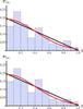Fig. 1 Probability distribution, , of the impact parameter (p). The results of MCs observed by WIND at 1 AU and fitted by the Lundquist model (Lepping & Wu 2010; Lepping et al. 1990) are shown with a histogram having 10 bins of p. Black curve: a linear fit to the histogram. Red curve: the Gaussian function derived by Lepping & Wu (2010). The histogram in the top panel has 100 MCs, while the one in the bottom panel is restricted to the 74 best observed MCs (quality 1, 2).

A variety of alternative models has been proposed for MCs. Keeping the cylindrical symmetry, a diversity of non-linear force-free field models is also possible (see Sect. 3.1). One possibility has a uniform twist within the cross section (e.g., Dasso et al. 2003, 2005a; Farrugia et al. 1999). Also, several non-force-free models have been applied, using different shapes for their cross sections (e.g., Cid et al. 2002; Hidalgo 2011; Hidalgo et al. 2002; Mulligan et al. 1999). So far, even if a given model has been shown to better fit the data of a few MCs than other models, this conclusion has not been extended to a large set of MCs. Indeed, the typical internal structure (e.g., the twist profile) of MCs is still not precisely known.

Another approach is to include the curvature of the flux rope axis by developing toroidal models (Marubashi 1997; Marubashi & Lepping 2007; Owens et al. 2012; Romashets & Vandas 2003, 2009). This approach is especially needed when a leg of the flux rope is crossed (i.e., when the spacecraft trajectory is close to the local flux rope axis direction). In this case, the inclusion of the axis curvature can strongly change both the deduced axis orientation and the impact parameter (Marubashi et al. 2012). Such leg crossings are typically characterized by a long-duration MC with a complex rotation profile of the magnetic field and a low angle between the solar radial direction and the flux rope axis (known as the cone angle). The frequency of such cases is small in the dataset of Lepping & Wu (2010) with, for example only 6 of 98 MCs with a cone angle below 30° and none for the 67 MCs of quality 1 and 2 (as defined in their paper). Then, we consider only local models of MCs with a straight axis as they have fewer free parameters than toroidal models.

One major unknown is the extension of the MC cross section. A way to deduce it is to solve the non-linear force-free equations by a direct numerical integration with the measured vector magnetic field as boundary conditions. This approach only supposes a magnetostatic field invariant by translation along the straight axis (Hu & Sonnerup 2002; Sonnerup et al. 2006). The method was tested successfully with MCs crossed by two spacecraft (Kilpua et al. 2009; Liu et al. 2008; Möstl et al. 2009a). The results depend on the MC studied, ranging from nearly round to elongated cross sections (Farrugia et al. 2011; Hu et al. 2005; Isavnin et al. 2011; Liu et al. 2008; Möstl et al. 2009a,b). The main limitation of this kind of approach is that it solves an ill-posed problem: the integration of an elliptic partial differential equation from a part of the boundary of the domain. The results can indeed be strongly affected by the time resolution and the range of the data used, as well as by the method implemented to stabilize the integration.

The short review above shows a large variety of flux rope models. If the MC data of Lepping & Wu (2010) had been fitted by one of these models, how would the estimated impact parameter, p, have been affected? Said differently, how model dependent is the MC distribution shown in Fig. 1? Moreover, how strongly do selection effects, e.g., on the amount of magnetic field rotation or field strength, affect such a distribution? We analyzed these issues for a large set of MCs by studying a variety of force-free field models (as the plasma-β is typically around 0.1 in MCs). The meaning of the main parameters used throughout the paper is summarized in Table 1.

The observation results and the fitting method are summarized in Sect. 2. In Sect. 3, we investigate the effect of a broad spectrum of magnetic field profiles ranging from flat to peaked around the axis, keeping a circular cross section. In Sect. 4, we mostly investigate the effect of the cross section elongation on models having elliptical cross sections. We also analyze the effect of bending the cross section to a “bean shape”. We conclude that p is most affected by the aspect ratio of the cross section. Then, in Sect. 5, we deduce a distribution of the aspect ratio compatible with the results of Lepping & Wu (2010). Next, in Sect. 6, we further analyze the MCs according to their global properties and show that some sets of MCs have a relatively round cross section. Finally, we conclude by summarizing our results and, in particular, answering the question set in the title of this paper (Sect. 7).

2. Observations and fitting method

2.1. Observed probability distribution of the impact parameter

We used the results of the Lundquist model fitted to MCs observed at 1 AU by the WIND spacecraft from February 1995 to November 2007¹. The list from 13 Dec., 2011 contains the results of 120 MCs. However, we restrict the list to 110 MCs by removing the cases where the handedness could not be determined (flag f in the list) or the fitting convergence was not achieved (flag F). Next, we examined the cone angle β which is the angle between the MC axis (found by the Lundquist fit) to the solar radial direction (X-axis in GSE coordinates). We considered a folded angle, so β was in the range [0°,90°]. Since the data obtained in the cases of MC leg crossing were the most difficult to analyze, making the fit results from cases with small β angle the most uncertain (Sect. 1), we limit the study to β > 30°. This restricted the MC sample to 103 MCs. Finally, there were 3 MCs with an impact parameter p > 1 (so a fitted flux rope extending beyond the first zero of the axial field in the Lundquist model). After we removed these suspicious cases, which comprised the worst class (quality 3, as defined in Lepping & Wu 2010), 100 MCs remained. One can even be more strict on the selection criteria. An extreme case is to select only the best cases (quality 1), with the limitation that the statistics is then restricted to 19 MCs. A less extreme case is to select the best and good cases (quality 1 and 2), yielding 67 MCs. We verified that our results were not significantly affected by the group of MC selected.

Lepping & Wu (2010) found that the number of MCs detected decreases rapidly with p. The same result is shown in Fig. 1 for the 100 MCs selected and a bin size of Δp = 0.1. Very close results are obtained if we restrict the analysis to the best observed MCs (quality 1 and 2). We define a probability of detection by normalizing the sum of the bin counts to 1. This allows the comparison between the results obtained with different sets of MCs and the model predictions. The Gaussian function shown in Fig. 1 (red curve) is a fit of the distribution as given by Eq. (A1) of Lepping & Wu, with b = 0 and σ = 0.407. It also fits well both sets of MCs shown in Fig. 1. The observed distribution can also be fitted with a linear function without significant difference with a Gaussian function (taking into account the statistical fluctuations).

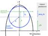Fig. 2 Drawing defining the geometry parameters for a spacecraft crossing an MC. The fit of the Lundquist field is schematized by the blue circle, while the black ellipse delimitates the half extension of the MC boundary. In this figure, we scale the drawing with the semi-minor axis of the ellipse set to unity. The true impact parameter, y/b, is larger than p.

Fig. 3 Examples of circular models (black dots) least square fitted with the Lundquist field (red curves). Three non-linear force-free models (n = 0.1,0.5,2) are selected to represent strong departure to the Lundquist field (n = 1). The true impact parameter, y/b, is either null (left) or large (right). Bz is the axial field component, and By is the azimuthal field component for y = 0. The field strength of the model on the axis, Baxis, is normalized to 1.

2.2. Flux rope fit with the Lunquist field

Models are used to simulate flux rope crossings, providing synthetic observations that are analyzed as MCs, thus following the classical procedure of Lepping et al. (1990). These synthetic models can be chosen as circular or elliptic, and the half extension of such a structure is given in black in Fig. 2. Then, the bias in the fits are analyzed. The simulated trajectory is set at a distance y parallel to the x-axis, because of the invariance in the z direction of the models, the same B would be obtained along a trajectory inclined on the flux rope axis. The true impact parameter is y/b, where b is the size of the structure in the y-direction (Fig. 2). The synthetic observations are fitted with a linear force-free model, the classical Lundquist solution (Lundquist 1950), which is in cylindrical coordinates: 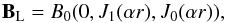${{B}}_{\mathrm{L}}\mathrm{=}{\mathit{B}}_{\mathrm{0}}\mathrm{\left(}\mathrm{0}\mathit{,}{\mathit{J}}_{\mathrm{1}}\mathrm{\right(}\mathit{\alpha r}\mathrm{\left)}\mathit{,}{\mathit{J}}_{\mathrm{0}}\mathrm{\right(}\mathit{\alpha r}\mathrm{\left)}\mathrm{\right)}\mathit{,}$(1)where α is associated with the first zero of Bz, B₀ is the axial field strength, and J_m is the ordinary Bessel function of order m. The fit of Eq. (1) to the synthetic observations provides an estimation of y, called y_L, with an origin not necessarily located on the true flux rope axis (Fig. 2). Then, the Lundquist fit provides the estimated impact parameter p = y_L/R, where R is the estimated flux rope radius (defined for B_z = 0).

The B_L field is fitted to the synthetic observations B_obs by minimizing the function dev defined by 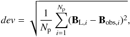$\mathit{dev}\mathrm{=}\sqrt{\frac{\mathrm{1}}{{\mathit{N}}_{\mathrm{p}}}\sum _{\mathit{i}\mathrm{=}\mathrm{1}}^{{\mathit{N}}_{\mathrm{p}}}\mathrm{(}{{B}}_{\mathrm{L}\mathit{,i}}\mathrm{-}{{B}}_{\mathrm{obs}\mathit{,i}}{\mathrm{)}}^{\mathrm{2}}}\mathit{,}$(2)where N_p is the number of points in the synthetic observations, B_obs is related with y/b, and B_L is related to p. Providing that N_p is large enough (i.e., N_p > 20), the results of the fits are insensitive to the value of N_p, which is to be expected because the synthetic observations are well resolved with such N_p values. Since the orientation of B_obs in MCs follows that of B_L better than the magnetic field magnitude, Lepping et al. (1990) fitted B_obs with B_L with a two-step procedure. In the first step, both B_obs and B_L norms are normalized to unit at each point before minimizing dev. Then, in the second step, the full fields are considered and dev is minimized by only changing the axial field strength B₀. From synthetic Lundquist fields, Gulisano et al. (2007) also concluded that fitting to normalized B_obs gives better estimation of the real orientation of the MC axis.

Compared to real MC observations, the models provide synthetic observations with no internal structures and with known axis orientation and boundaries. The exploration of the effect of perturbations on B and on various axis orientations and boundaries could be realized in the line of the following exploration of the parameter space (e.g., the parameters defining the shape of the cross section). However, we chose to limit the exploration to the global structure of the flux ropes (i.e., the magnetic field repartition and the cross section shape) as such a structure is expected to have a major effect on the estimated impact parameter. Then, in the above first step, the minimization is realized by changing p and α (because both the axis orientation and the flux rope boundaries, set at B_z = 0, are known and fixed).

3. Detecting circular flux ropes

In this section, we analyze a series of circular force-free fields in order to test if the impact parameter could be biased by the choice of the model with the classical analysis of Lepping et al. (1990).

3.1. Force-free models

Frequently, the magnetic structure of an MC is locally approximated by a straight flux rope invariant along its axis (Sect. 1). We use below an orthogonal frame, called the MC frame, with coordinates (x,y,z). The z direction is along the MC axis. Because B is independent of z and ∇·B = 0, the implication is that one can write the magnetic field components orthogonal to the symmetry axis B_x = ∂A/∂y and B_y = − ∂A/∂x, where A(x,y) is the magnetic flux function. The force-free field condition implies 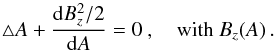$\mathrm{△}\mathit{A}\mathrm{+}\frac{\mathrm{d}{\mathit{B}}_{\mathit{z}}^{\mathrm{2}}\mathit{/}\mathrm{2}}{\mathrm{d}\mathit{A}}\mathrm{=}\mathrm{0}\mathit{,}\mathrm{with}{\mathit{B}}_{\mathit{z}}\mathrm{\left(}\mathit{A}\mathrm{\right)}\hspace{0.17em}\mathit{.}$(3)A series of non-linear force-free fields are generated by 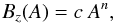${\mathit{B}}_{\mathit{z}}\mathrm{\left(}\mathit{A}\mathrm{\right)}\mathrm{=}\mathit{c}{\mathit{A}}^{\mathit{n}}\mathit{,}$(4)where c and n > 0 are independent of x,y,z. Typically, the flux rope boundary is set at a location where B_z = 0, which can be set for A = 0 without losing generality. We normalized the cross-section extension to the half of its maximal value in the x-direction (Fig. 2). Its half maximal extension in the y-direction is then the aspect ratio, b, set to b = 1 in this section (i.e., circular shape). The flux rope axial field is called B_axis.

Since we consider circular flux ropes in this section, Eq. (3) reduces to a differential equation of second order with the radius ($\sqrt{{\mathit{x}}^{\mathrm{2}}\mathrm{+}{\mathit{y}}^{\mathrm{2}}}$). It is solved by a numerical integration using a shooting method (e.g., Press et al. 1992,p. 746) applied to the resonance problem set by Eqs. (3), (4) and the three boundary conditions A(0) = 1, [dA/dr] (0) = 0, and A(1) = 0 (corresponding respectively to an azimuthal flux normalized to 1, a regular field on the axis, and to B_z = 0 at the boundary). We select the lowest eigenvalue c to have models with an axial field vanishing only at the boundary as present in most MCs. For n = 1, the field is a linear force-free field and c = α (as defined by Eq. (1)). Finally, the field strength on the axis can be scaled to any desired B_axis value.

The axial electric current density is ${\mathit{j}}_{\mathit{z}}\mathrm{=}\mathrm{-}\mathrm{△}\mathit{A}\mathit{/}{\mathit{\mu }}_{\mathrm{0}}\mathrm{=}\mathit{n}{\mathit{c}}^{\mathrm{2}}\mathrm{\left(}\mathit{A}\mathrm{\right(}\mathit{x,y}\mathrm{)}{\mathrm{)}}^{\mathrm{2}\mathit{n}\mathrm{-}\mathrm{1}}\mathit{/}{\mathit{\mu }}_{\mathrm{0}}\mathit{,}$(5)where μ₀ is the permeability of the free space. For n = 0.5, j_z is uniform, while for n > 0.5, j_z decreases from the axis to the boundary (where A = 0, so j_z = 0). Finally, for n < 0.5, j_z is singular at the boundary (presence of a current sheet).

The value of n also determines the spatial variation of B. This is illustrated in the left-hand panels of Fig. 3. Because n is increased, the magnetic field strength becomes more concentrated around the axis and, near the boundary for n > 0.5, the azimuthal field (=| B_y | at y = 0) is a decreasing function of the radius (=$\sqrt{{\mathit{x}}^{\mathrm{2}}\mathrm{+}{\mathit{y}}^{\mathrm{2}}}$) over a larger radius range. The case n = 2, Fig. 3e, is an extreme case for an MC. In contrast, as n decreases, the profile of the magnetic field strength flattens. For n = 0.5, the azimuthal field is linear with radius, while for n < 0.5, it increases more sharply near the boundary as n is decreased. The case n = 0.1 is another extreme case for an MC. The Lundquist model fits the different models relatively well, except in extreme cases (e.g., n = 2 case, Fig. 3e, f), even for large impact parameters (e.g., see the case y/b = 0.9 in Fig. 3b, d).

3.2. Information provided by the Lundquist fit

The results of Fig. 4a show that y/b is relatively well estimated by p for all the range of n values relevant to MCs. The extreme case n = 0.1 has very similar results to the case n = 0.25, so it is not shown. All cases with n < 1 have p only slightly lower than y/b, so that the observed distribution probability (in function of p) would only be slightly compressed toward lower p values compared to the original distribution probability (in function of y/b). In contrast, all cases with n > 1 would introduce a bias opposite to those observed since p > y/b (Fig. 1). We conclude that the deviation around y/b = p (green curve, n = 1 in Fig. 4a) cannot explain the strong decrease of the probability to observe an MC with moderate and large p values seen in Fig. 1.

The axial field of the model, set to B_axis = 1, is also well recovered with the fitted parameter B₀ of the Lundquist field (Fig. 4b). Only large differences (>20%) are obtained for glancing encounters (p, so y/b, close to 1) or peaked magnetic field profiles (e.g., n = 2).

Next, we normalized the deviation, Eq. (2), by ⟨ B⟩, the average of the field strength along the simulated trajectory. Figure 4c shows that the deviation of the fit to synthetic data is relatively small unless extreme cases are considered (e.g., n = 2, see also Fig. 3). It is important to notice that dev/ ⟨B⟩ is not a secure indicator of the precision of the fitted parameters: for example B_L fits well the synthetic observations for large p with a low dev/ ⟨B⟩ value (Figs. 3, 4), while the fitted parameters are more biased (e.g., B₀) and/or unprecised for these glancing encounters.

Finally, Lepping & Wu (2010) found that ⟨ B⟩ /B₀(p) from the analyzed MCs followed very well the expected relation from the Lundquist field, except from a slight shift in ordinate (see their Fig. 5). This shift could be explained by n ≈ 0.7–0.8 (Fig. 4d). This is an indication that the typical field in MCs is between a linear force-free field and a field with constant axial current density. This result is in the same line of those obtained by Gulisano et al. (2005), where crude approximations were done (assuming circular cross section, zero impact parameter, and the orientation of the main axis are given only from the minimum variance method). They found clues in favor of magnetic configurations between linear force-free field and constant current models.

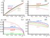Fig. 4 a) Dependence of the true impact parameter, y/b, b) the fitted Lundquist field strength on the axis, B0, c) the normalized deviation, dev/ ⟨B⟩, and d) the mean field magnitude ⟨ B⟩ normalized to B0 in function of the impact parameter, p, found by fitting the Lundquist field to the models. The parameter n describes the profile of the axial component of the magnetic field and electric current, see Eqs. (4), (5).

3.3. Is there a significant selection effect with p?

The rotation angle of the magnetic field along the simulated trajectory is weaker as the impact parameter increases (Fig. 5). Since an important field rotation is a key ingredient in defining an MC, a too weak rotation angle could lead to no MC detection, and thus a bias in the probability distribution in function of p. As in Lepping & Wu (2010), we analyzed the rotation angle of B in the plane orthogonal to the flux rope axis by taking the angle formed by B at each of the two boundaries (hereafter noted ω). Because they averaged the observed B over one hour (their Fig. 3B), the modeled B is averaged over 5% of the crossing length near the boundaries in order to be comparable to their observations. For a typical MC duration of 20 h, this implies an average over 1 h, so that our results are directly comparable to their Fig. 3B.

For the case n = 1, the synthetic data are derived from the Lundquist field, like the fitting field; it implies that the rotation angle has a simple expression, 2arccos(p), which is nearly identical to the green curve in Fig. 5 (the differences are only due to the small averaging performed near the boundaries). Finally, we found that a broad range of n values is compatible with their results (Fig. 5), so that the amount of B rotation angle does not allow to select between different models. This result is confirmed in Sects. 4 and 5.

Is there a severe selection effect with the amount of rotation angle in observed MCs? In fact, for a rotation angle lower than 30°, no MC is observed (Fig. 5). Four MCs are observed with a rotation angle as low as ≈ 50° or less, showing that MCs with a low rotation angle can be detected. This value of ω corresponds to p > 0.9 with the above models, so that a selection effect on MCs with a low B rotation angle cannot explain the progressive decrease of the detection probability of MCs with p (Fig. 1). A way out would be to argue that significant B structures are frequently present within MCs, especially close to the boundary (i.e., for large p values), so that they can mask the lower rotation cases even more. However, an important rotation angle, ω > 90°, is still present for p ≈ 0.7, both for MCs and simulated flux ropes (Fig. 5). Then, it is very unlikely that the presence of B structures in MCs can decrease the probability of detection by a factor 3 to 4 for p ≈ 0.7 (Fig. 1). It implies that a selection effect on rotation angle cannot explain the observed probability. In the same line, B₀ remains close to B_axis (Fig. 4b), so that a selection effect on the field strength is expected to be weak for flux rope with a nearly circular cross section.

We conclude that the explored circular models cannot explain the observations (Fig. 1).

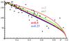Fig. 5 Dependence of the rotation angle, ω, of the magnetic field component orthogonal to the axis in function of the impact parameter, p, found by fitting the Lundquist field to circular models (Eqs. (3), (4)). The dots are the results obtained by Lepping & Wu (2010) for 65 MCs (see their Fig. 3B).

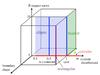Fig. 6 Drawing defining the regions of the parameter space explored. The red line indicates the circular models analyzed in Sect. 3. The MC boundary is elliptical for the blue region and is deformed to a bean shape in the green region. The two blue lines indicate the elliptical models analyzed in Sect. 4. Finally, the purple line indicates an extreme case where the MC boundary is rectangular. n defines the axial electric current and magnetic field component (Eqs. (3), (4)). A cross section elongated orthogonally to the spacecraft trajectory has b > 1 (Fig. 2).

4. Detecting flux ropes with elongated cross section

In this section, we explore mainly the effects of the flux rope boundary shape. An elliptical boundary is described by its aspect ratio b (b > 1 means that the cross section is elongated orthogonally to the MC trajectory, Fig. 2). We also consider bent cross sections in Sect. 4.5, which are described by an extra parameter called a. A rectangular cross section is also considered (it is an extreme case). These different types of cross sections allow exploration of the space of parameters (Fig. 6) with models depending on a set of parameters (a,b,n).

4.1. Expected effect of the cross section aspect ratio

Gulisano et al. (2007) have shown that the ratio r_Bx = ⟨B_x⟩ / ⟨B⟩ is a function of the true impact parameter y/b for a variety of circular models (⟨ ⟩ means averaging along the spacecraft trajectory within the MC). Démoulin & Dasso (2009) have extended this relationship for linear force-free models with various boundary shapes (see their Fig. 10). For an elliptical boundary, this relationship is summarized as r_Bx(y/b,b,n = 1). This applies in particular to the Lunquist field (b = 1) and is simply summarized as r_Bx,L(y/b) ≡ r_Bx(y/b,b = 1,n = 1).

Next, a similar ⟨ B_x⟩ / ⟨B⟩ is expected when B_L is fitted to B (since B_L approaches the best possible B). Setting the equality r_Bx(y/b,b,n = 1) = r_Bx,L(p) provides a relation p(y/b,b). For a fixed y/b value, the derivation of this relation implies dp/db = (dr_Bx/db)/(dr_Bx,L/dp). Since r_Bx is a decreasing function of b for a fixed y/b and r_Bx,L is an increasing function of p (Démoulin & Dasso 2009), this implies that p is a decreasing function of b.

Finally, with the magnitude of change of r_Bx with b found in Fig. 10 of Démoulin & Dasso (2009), the value of b is expected to strongly affect the estimated p value. As a result, it is expected to strongly bias the MC probability distribution (Fig. 1). This expectation is tested below by fitting with B_L a variety of models with elongated cross section.

Fig. 7 Examples of two elliptical models (n = 0.5,1, black dots) least square fitted with the Lundquist field (red curves) for a large true impact parameter, y/b = 0.9. Bz is the axial field component, and By is the field component both orthogonal to the simulated trajectory and to the flux rope axis.

4.2. Models with elongated cross section

We explore the space of parameters mainly with analytical models as summarized in Fig. 6. The emphasis is set on the aspect ratio b since it was found to be the most important parameter affecting p (for a fixed y/b). We first analyze the model of Vandas & Romashets (2003), who derived an analytical solution of a linear force-free field (n = 1) contained inside an elliptical boundary (so generalizing B_L).

A numerical extension of the above model to cross sections with a bent (bean-like) shape was analyzed by Démoulin & Dasso (2009). They also consider the limit case of a rectangular cross section. It has a simple analytical expression for a linear force-free field (n = 1); see their Eq. (14) while their Eq. (15) should be ${\mathit{\alpha }}_{\mathrm{R}}\mathrm{=}\mathit{\pi }\mathit{/}\mathrm{2}\sqrt{\mathrm{1}\mathrm{+}{\mathit{b}}^{\mathrm{2}}}\mathit{/}\mathit{b}$.

Finally, even if we have shown in Sect. 3 that n has a small effect on circular cross sections, we also consider the force-free field with n = 0.5 and an elliptical cross section $\mathrm{\left(}{\mathit{B}}_{\mathit{x}}\mathit{,}{\mathit{B}}_{\mathit{y}}\mathit{,}{\mathit{B}}_{\mathit{z}}\mathrm{\right)}\mathrm{=}\left(\mathrm{-}\frac{\mathit{y}}{\mathit{b}\sqrt{\mathrm{1}\mathrm{+}{\mathit{b}}^{\mathrm{2}}}}\mathit{,}\frac{\mathit{x}\mathit{b}}{\sqrt{\mathrm{1}\mathrm{+}{\mathit{b}}^{\mathrm{2}}}}\mathit{,}\sqrt{\mathrm{1}\mathrm{-}{\mathit{x}}^{\mathrm{2}}\mathrm{-}{\left(\frac{\mathit{y}}{\mathit{b}}\right)}^{\mathrm{2}}}\right)\mathrm{·}$(6)

4.3. Effect of the aspect ratio

As the aspect ratio b increases, more significant deviations between the synthetic observations of the modeled B and the fitted B_L are present. For example, Fig. 7 shows two extreme cases with b = 4 and y/b = 0.9 (similar fits are obtained with lower y/b values). For both cases the field rotation angle, ω, is about 120°, and thus large enough to be detected. However, using at typical value of B_axis = 20 nT at 1 AU, such a flux rope would not be detected for n = 1. However, for n = 0.5, it would since the respective mean magnetic field strength along the simulated trajectory is ≤0.8 and ~9 nT (compare to a typical SW field ≈5 nT).

As expected in Sect. 4.1, the aspect ratio b has a strong effect on the estimated impact parameter p (Fig. 8a, c). This effect is much stronger than the effect of n for circular flux ropes (Fig. 4a). The results obtained for n = 1 and a rectangular boundary are similar (so not shown) to the results for n = 0.5 and an elliptical boundary. All these results imply that p is systematically biased to a lower value than the true impact parameter y/b, which strongly increases as b is larger.

As with circular models (Sect. 3.2), the quality of the fit of B_L to the synthetic data (thus a low value of dev/ ⟨B⟩) cannot be used to estimate the quality of the derived fitted parameters, in particular of p. Indeed, even small values of dev/ ⟨B⟩ are present for large p values (Fig. 8b, d), where p is the most biased compared with y/b (Fig. 8a, c). Moreover, dev/ ⟨B⟩ has only a small dependence on b for n = 0.5, while p has a strong dependence on b. We conclude that the value of dev/ ⟨B⟩ is not a reliable way to qualify the best fitting model.

As the aspect ratio b is increased, the flux rope is stretched in the y direction, so one expects an increase of B_y at the expense of B_x and thus an increase of the field rotation angle ω. In the models shown here, this enhanced rotation angle is mainly present for the elliptical case with n = 1 (Fig. 9b). For the two other models, the rotation angle is almost independent of b (Fig. 9a, c).

With a larger b value, the magnetic field can expand further away in the y direction, implying lower field strength (see, e.g., Fig. 5 of Démoulin & Dasso 2009). The fit of B_L to this weaker field leads to a lower B₀ (much lower than B_axis). Then, we found that B₀ is a faster decreasing function of p for larger b values. By contrast, ⟨ B⟩ /B₀ is found to be almost independent of b and more generally of the boundary shape. Then, the slightly higher value of ⟨ B⟩ /B₀ for MCs than for a Lundquist field, as found by Lepping & Wu (2010) in their Fig. 5, is mainly related to the B_z(A) relation, and in particular to n, Eq. (4), as found at the end of Sect. 3.2.

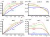Fig. 8 Dependence of the true impact parameter, y/b, and of the normalized deviation, dev/ ⟨B⟩ in function of the fitted impact parameter p, found by fitting the Lundquist field to elliptical boundary models. The parameter n describes the profile of the axial current (Eqs. (3), (4)).

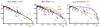Fig. 9 Dependence of the rotation angle, ω, of the magnetic field component orthogonal to the axis in function of the impact parameter, p, found by fitting the Lundquist field to two models with an elliptical boundary a), b) and one with a rectangular boundary c). The dots are the results obtained by Lepping & Wu (2010) for 65 MCs (see their Fig. 3B).

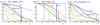Fig. 10 Probability distribution of the impact parameter, , deduced from various models and a uniform probability distribution of y/b. The thin curves are without selection effect and the thick curves are for ⟨ B⟩ /Baxis > 0.25 and a magnetic field rotation angle greater than 90°. The dashed black curve is a Gaussian function fitted to observations (Fig. 1).

4.4. Expected observed distribution of impact parameter

The above bias on the estimated impact parameter, p, has important implications for the observed probability distribution (e.g., Fig. 1). More precisely, let us consider MC models with the same physical characteristics and observing bias (called , which defines a set of five parameters, see Table 1). The simulated crossing is set at y/b with a distribution P(y/b). The models present in the interval [y/b,y/b + d(y/b)] are mapped to the interval [p,p + dp] with the Lundquist fit. The two probability distributions are related by $\mathrm{𝒫}\mathrm{\left(}\mathit{p,}\mathrm{𝒞}\mathrm{\right)}\mathrm{d}\mathit{p}\mathrm{=}\mathit{P}\mathrm{(}\mathit{y}\mathit{/}\mathit{b}\mathrm{)}\mathrm{d}\mathrm{(}\mathit{y}\mathit{/}\mathit{b}\mathrm{)}\mathit{.}$(7)Moreover, some flux ropes could not be recognized as MCs because the crossing was too close to the flux rope border. We include two important selection effects: a too weak field strength and a too low rotation angle of the magnetic field. Other selection effects are associated to the presence of strong distortions, especially present when two MCs are interacting (e.g., Dasso et al. 2009; Lugaz et al. 2005a; Wang et al. 2003). Our models cannot take into account these relatively rare cases of MCs in interaction. For isolated MCs, the distortions close to the boundary are expected to be the strongest (weaker magnetic field and stronger effect of the surroundings, e.g., Lepping et al. 2007). Therefore, we select a relatively large minimum rotation angle, ω_min = 90°, while MCs are detected in observations with a minimum rotation angle of ≈40° (Fig. 9). The flux rope can also be missed if its magnetic field strength is too weak. We select cases with ⟨ B⟩ /B_axis ≥ r_Bmin with typically r_Bmin = 0.25, since for a typical B_axis value of 20 nT this implies that ⟨ B⟩ is comparable to the typical field magnitude in the solar wind at 1 AU. Supposing a uniform distribution P(y/b) (see Sect. 1), and including the above selection effects in Eq. (7), the probability of detecting an MC is 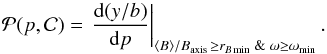$\mathrm{𝒫}\mathrm{\left(}\mathit{p,}\mathrm{𝒞}\mathrm{\right)}\mathrm{=}{\frac{\mathrm{d}\mathrm{(}\mathit{y}\mathit{/}\mathit{b}\mathrm{)}}{\mathrm{d}\mathit{p}}|}_{\mathrm{⟨}\mathit{B}\mathrm{⟩}\mathit{/}{\mathit{B}}_{\mathrm{axis}}\hspace{0.17em}\mathrm{\ge }{\mathit{r}}_{\mathit{B}\min }\mathrm{\&}\mathit{\omega }\mathrm{\ge }{\mathit{\omega }}_{\min }}\mathit{.}$(8)Within the studied models (Fig. 6) the weakest bias of p with increasing b is obtained for the linear force-free model, n = 1, with an elliptic cross section (Fig. 8c). It implies a moderate decrease of with p without selection effect (r_Bmin = ω_min = 0, see thin curves in Fig. 10b). The selection effect with ω is only present for large p values and its effect decreases with b (Fig. 9b). However, this model also has the weakest ⟨ B⟩ for large p values. It implies a strong selection effect for r_Bmin = 0.25, increasing with b (thick curves in Fig. 10b).

Increasing the axial currents (n = 0.5) or extending the cross section to a rectangular shape implies a stronger magnetic field for large p and thus a weaker selection effect. The selection effect with the field rotation angle also remains limited to large p values (Fig. 9a, c). Moreover, as b is increased, the strong decrease of d(y/b)/dp with p further reduces the selection effects (compare thin and thick curves in Fig. 10a, c). We conclude that the relation p(y/b) has generically a major effect on the observed MC distribution drawn in function of p.

Can we interpret the observed distribution (Fig. 1) as due to oblate cross sections? For the elliptic case with n = 1, none of the distributions with a fixed b and selection criteria are close to the observed distribution (Fig. 10b). However, a mixture of such distributions well could be, and this will be analyzed in Sect. 5. For the elliptic case with n = 0.5, is very close (i.e., within the error bars) to the observed distribution for b ≈ 2 (Fig. 10a), while for the rectangular boundary with n = 1, is also close to the observed distribution for b ≈ 1.5 (Fig. 10c).

4.5. Effect of a bent cross section

In some MHD simulations, the flux rope is strongly compressed in the propagation direction, such that its front region becomes relatively flat (e.g., Vandas et al. 2002). The cross section can even develop a bending of the lateral sides towards the front direction when its central (resp. lateral) parts move in a slow (resp. fast) solar wind (e.g., Riley et al. 2003; Manchester et al. 2004). Démoulin & Dasso (2009) have investigated the effects of bending the flux rope boundary to a bean-like shape. This bending is parameterized by the dimensionless parameter called a. Examples of computed fields with various a values are shown in their Figs. 3–5. Typically | a | needs to be larger as b increases to get a comparable bending.

Does bending of the flux rope cross section modify the probability distribution of flux rope detection, , versus the estimated parameter p? The effect of a value can be approximately derived from the relation r_Bx = ⟨B_x⟩ / ⟨B⟩ in function of y/b,a and b as summarized by the analytical expression of Eq. (31) of Démoulin & Dasso (2009). As in Sect. 4.1, a similar ⟨ B_x⟩ / ⟨B⟩ is expected for B and its fitted B_L field. Setting the equality r_Bx,L(p) = r_Bx(y/b,a,b) provides an estimation of p, named p_e(a,b,y/b), which is shown in Fig. 11 for a few a and b values.

We also compare the estimation p_e to the result of fitting B_L to B for a = 0, so an elliptical boundary (dashed black line). For b = 1, both curves are simply p = p_e = y/b (Fig. 11a), while for b > 1, there is good agreement up to large y/b values (Fig. 11b). Such a result could be extended to a > 0 by applying the Lundquist fit to the bent models developed by Démoulin & Dasso (2009). Then, the analytical expression p_e(a,b,y/b) provides an estimation of p for a broad range of { a,b,y/b } values. This result has a practical application: it provides a good initial guess of p (from observed r_Bx) for the non-linear fit of B_L to B (thus both avoiding starting in a wrong local well of dev, Eq. (2) and speeding up the computations).

Figure 11 shows that bending of the flux rope cross section, so increasing | a |, increases p for a given y/b. This is the opposite effect of increasing b (Fig. 8a, c). As seen in Eq. (8), this implies a bias toward increasing the probability of flux ropes for large p, which is the opposite of the observations (Fig. 1). It is also worth noting that | a | = 2 is already a very bent cross section (see Figs. 4, 5 of Démoulin & Dasso 2009) that we expect to be rarely present in observed MCs. We conclude that the effect of bending the cross section is expected to introduce only a weak bias to the estimated p value.

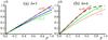Fig. 11 Approximate dependence of the true impact parameter, y/b, in function of the estimated impact parameter, p, for bent cross sections derived from Démoulin & Dasso’s (2009) results (derived from rBx, see text in Sect. 4.5). The bending increases with the dimensionless parameter a. Linear force-free models (n = 1, Eq. (4)) are shown for two aspect ratio b. The black dashed line is the relation found by fitting the Lundquist field to the elliptic (a = 0) model with n = 1.

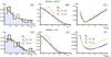Fig. 12 Probability distributions from Eq. (9) and P(b) from Eqs. (11), (13) for the minimum of dist(η,bmean) as defined by Eq. (10). of Fig. 1 is added in a), d). Two force-free elliptical models are shown: a)–c) n = 0.5 (constant current density), d)–f) n = 1 (linear force-free) for rBmin = 0.25 and ωmin = 0. The three P(b) functions, shown with three colors, imply similar results.

5. Distribution of the cross-section aspect ratio

In the previous section, we found that the probability distribution was most sensitive to the aspect ratio b. In this section, we use this property to constrain the probability distribution, P(b), of the aspect ratio b for the MCs observed at 1 AU. We end by exploring how P(b) depends on the MCs’ properties.

5.1. Method

In the following, we consider that the aspect ratio b is distributed according to the probability function P(b), while the other parameters in remain the same. Because of the small effect of a, see Sect. 4.5, we set a = 0. The expected probability of the impact parameter is the superposition of the contribution of each b values according to 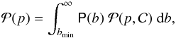$\mathrm{𝒫}\mathrm{\left(}\mathit{p}\mathrm{\right)}\mathrm{=}{\mathrm{\int }}_{{\mathit{b}}_{\min }}^{\mathrm{\infty }}\mathrm{P}\mathrm{\left(}\mathit{b}\mathrm{\right)}\mathrm{𝒫}\mathrm{\left(}\mathit{p,}\mathrm{𝒞}\mathrm{\right)}\mathrm{d}\mathit{b,}$(9)where and ${{}^{\mathrm{\int }}\mathit{b}_{\min }}_{\mathrm{\infty }}^{}\mathrm{P}\mathrm{\left(}\mathit{b}\mathrm{\right)}\mathrm{d}\mathit{b}\mathrm{=}\mathrm{1}$, while ${{}^{\mathrm{\int }}}_{\mathrm{0}}^{\mathrm{1}}\mathrm{𝒫}\mathrm{\left(}\mathit{p,}\mathrm{𝒞}\mathrm{\right)}\mathrm{d}\mathit{p}\mathrm{\le }\mathrm{1}$ since cases are missed with the selection on r_Bmin and ω_min.

Since P(b) is contributing through an integral to the distribution in Eq. (9) and (shown in Fig. 1) has important uncertainties due to the limited number of observed MCs, we can only derive a global behavior of P(b). For that, we limit the freedom of P(b) by selecting functions that depend on few parameters (${\mathit{b}}_{\mathrm{mean}}\mathit{,}{\mathit{b}}_{\mathrm{c}}^{\mathrm{\prime }}$) and minimize the distance, dist, between and 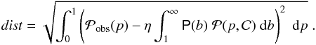$\mathit{dist}\mathrm{=}\sqrt{{\mathrm{\int }}_{\mathrm{0}}^{\mathrm{1}}{\left({\mathrm{𝒫}}_{\mathrm{obs}}\mathrm{\left(}\mathit{p}\mathrm{\right)}\mathrm{-}\mathit{\eta }{\mathrm{\int }}_{\mathrm{1}}^{\mathrm{\infty }}\mathrm{P}\mathrm{\left(}\mathit{b}\mathrm{\right)}\mathrm{𝒫}\mathrm{\left(}\mathit{p,}\mathrm{𝒞}\mathrm{\right)}\mathrm{d}\mathit{b}\right)}^{\mathrm{2}}\mathrm{d}\mathit{p}}\mathit{.}$(10)We introduce the parameter η in front of since is normalized with all the observed MCs (${{}^{\mathrm{\int }}}_{\mathrm{0}}^{\mathrm{1}}{\mathrm{𝒫}}_{\mathrm{obs}}\mathrm{\left(}\mathit{p}\mathrm{\right)}\mathrm{d}\mathit{p}\mathrm{=}\mathrm{1}$), while each is normalized to all the cases. Since we cannot also normalize to all cases, we leave η as a free parameter. It is expected to be around 1 since the selection biases are expected to be small (Sect. 4).

The generic cross section shape of MCs is mostly unknown since the only shape determinations were done with a Grad-Shafranov reconstruction technique or by fitting the elliptical linear force-free model on a few MCs (see Sect. 1). The cross section has the tendency to be round (b ≈ 1) because of the magnetic tension and the typically low plasma β found in MCs. However, the large pressure of the MC sheath tends to elongate the cross section orthogonally to the MC mean velocity, so b > 1. Then, we set a minimum value for b as b_min = 1. Indeed, the MCs with b < 1 cannot be too numerous, otherwise more MCs with large p would be observed (because for b < 1 the bias of p(y/b) is the reverse of b > 1).

We first select a simple linear function for P(b) 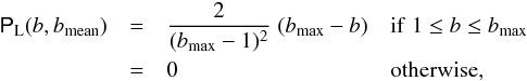$\begin{array}{ccc}{\mathrm{P}}_{\mathrm{L}}\mathrm{\left(}\mathit{b,}{\mathit{b}}_{\mathrm{mean}}\mathrm{\right)}& \mathrm{=}& \frac{\mathrm{2}}{\mathrm{(}{\mathit{b}}_{\max }\mathrm{-}\mathrm{1}{\mathrm{)}}^{\mathrm{2}}}\mathrm{(}{\mathit{b}}_{\max }\mathrm{-}\mathit{b}\mathrm{)} \mathrm{if}\mathrm{1}\mathrm{\le }\mathit{b}\mathrm{\le }{\mathit{b}}_{\max }\\ & \mathrm{=}& \mathrm{0}\mathrm{otherwise}\mathit{,}\end{array}$(11)where the coefficient in front of (b_max − b) is computed from the normalisation ${{}^{\mathrm{\int }}}_{\mathrm{1}}^{{\mathit{b}}_{\max }}{\mathrm{P}}_{\mathrm{L}}\mathrm{\left(}\mathit{b,}{\mathit{b}}_{\mathrm{mean}}\mathrm{\right)}\mathrm{d}\mathit{b}\mathrm{=}\mathrm{1}$, and ${\mathit{b}}_{\mathrm{mean}}\mathrm{=}{\mathrm{\int }}_{\mathrm{1}}^{{\mathit{b}}_{\max }}\mathit{b}{\mathrm{P}}_{\mathrm{L}}\mathrm{\left(}\mathit{b,}{\mathit{b}}_{\mathrm{mean}}\mathrm{\right)}\mathrm{d}\mathit{b}\mathrm{=}\frac{{\mathit{b}}_{\max }\mathrm{+}\mathrm{2}}{\mathrm{3}}\mathrm{·}$(12)As a second possibility for P(b) we select a Gaussian distribution, limited to b ≥ 1 $\begin{array}{ccc}{\mathrm{P}}_{\mathrm{G}}\mathrm{\left(}\mathit{b,}{\mathit{b}}_{\mathrm{mean}}\mathit{,}{\mathit{b}}_{\mathrm{c}}^{\mathrm{\prime }}\mathrm{\right)}& \mathrm{=}& \\ \mathrm{with} \mathit{f}& \mathrm{=}& \sqrt{\frac{\mathrm{2}}{\mathit{\pi }}}\frac{\mathrm{1}}{\mathrm{(}\mathrm{1}\mathrm{+}\mathrm{erf}\mathrm{(}{\mathit{b}}_{\mathrm{c}}^{\mathrm{\prime }}\mathrm{\left)}\mathrm{\right)}\mathit{\sigma }}\mathit{,}\\ {\mathit{b}}_{\mathrm{c}}^{\mathrm{\prime }}& \mathrm{=}& \mathrm{(}{\mathit{b}}_{\mathrm{c}}\mathrm{-}\mathrm{1}\mathrm{)}\mathit{/}\mathrm{\left(}\sqrt{\mathrm{2}}\mathit{\sigma }\mathrm{\right)}\mathit{,}\\ {\mathit{b}}_{\mathrm{mean}}& \mathrm{=}& \sqrt{\mathrm{2}}\mathit{\sigma }\left({\mathit{b}}_{\mathrm{c}}^{\mathrm{\prime }}\mathrm{+}\frac{\exp \mathrm{(}\mathrm{-}{{\mathit{b}}^{\mathrm{\prime }}}_{\mathrm{c}}^{\mathrm{2}}\mathrm{)}}{\sqrt{\mathit{\pi }}\mathrm{[}\mathrm{1}\mathrm{+}\mathrm{erf}\mathrm{(}{\mathit{b}}_{\mathrm{c}}^{\mathrm{\prime }}\mathrm{\left)}\mathrm{\right]}}\right)\mathrm{+}\mathrm{1}\mathit{,}\end{array}$(13)where erf is the error function. The coefficient f was computed from the normalisation ${{}^{\mathrm{\int }}}_{\mathrm{1}}^{\mathrm{\infty }}{\mathrm{P}}_{\mathrm{G}}\mathrm{\left(}\mathit{b,}{\mathit{b}}_{\mathrm{mean}}\mathit{,}{\mathit{b}}_{\mathrm{c}}^{\mathrm{\prime }}\mathrm{\right)}\mathrm{d}\mathit{b}\mathrm{=}\mathrm{1}$. The parameter b_mean is the mean value of P_G, restricted to b ≥ 1. The freedom of P_G is expressed in function of $\mathrm{\left\{}{\mathit{b}}_{\mathrm{mean}}\mathit{,}{\mathit{b}}_{\mathrm{c}}^{\mathrm{\prime }}\mathrm{\right\}}$ rather than with the usual parameters of a Gaussian distribution { b_c,σ } (Eq. (13)) in order to easily compare our results with the linear distribution P_L (Eq. (11)). Moreover, as shown below, b_mean value is the most stable result deduced from minimizing the function dist (Eq. (10)). Therefore, we set the parameter b_mean in both distributions. For a given b_mean, the normalized parameter ${\mathit{b}}_{\mathrm{c}}^{\mathrm{\prime }}$ determines the location of the maximum of P_G and the spread of the distribution as follows. The probability at b = 1 divided by the maximal one, at b = b_c, is simply $\exp \mathrm{(}\mathrm{-}{{\mathit{b}}^{\mathrm{\prime }}}_{\mathrm{c}}^{\mathrm{2}}\mathrm{)}$. Therefore, ${\mathit{b}}_{\mathrm{c}}^{\mathrm{\prime }}$ describes how much the function P_G is peaked (${\mathit{b}}_{\mathrm{c}}\mathrm{=}{\mathit{b}}_{\mathrm{c}}^{\mathrm{\prime }}\mathit{\sigma }\sqrt{\mathrm{2}}\mathrm{+}\mathrm{1}$, then for ${\mathit{b}}_{\mathrm{c}}^{\mathrm{\prime }}\mathrm{=}\mathrm{0}$, its maximum is at b = 1, while it is more peaked toward b > 1 as ${\mathit{b}}_{\mathrm{c}}^{\mathrm{\prime }}$ increases).

5.2. Probability distribution of aspect ratio: P (b)

In this section, for a given (Fig. 1), the function dist(η,b_mean), defined by Eq. (10), is minimized. We provide typical results for P(b).

The function dist(η,b_mean) has a well-defined global minimum in all explored cases, see e.g., Fig. 12c, f, where cuts through the minimum are shown in function of b_mean. For n = 0.5, the minima are nearly at the same location (η ≈ 0.91 ± 0.01, b_mean ≈ 2.29 ± 0.01 for the three P(b) functions shown), while for n = 1, η is larger (≈1.26 ± 0.06) and b_mean is more broadly distributed (from ≈2.2 to 3.4). For each n value, the derived are all very close and fit globally well the observations (Fig. 12a, d), with a comparable minimum of dist (≈0.036 for n = 0.5 and ≈0.035 for n = 1). There are still some differrences: for the case n = 1, is slightly lower than for both small and large p values (p < 0.3 and p > 0.7), while it is the opposite for the case n = 0.5 (Fig. 12a, d). It is an indication that n is typically between these values in MCs, in agreement with the result found for ⟨ B⟩ /B₀(p) at the end of Sect. 3.2.

5.3. Sensivity of P (b)

We compare below the results for P_L and P_G varying both the models (n, cross section shape) and the selection effects (r_Bmin and ω_min).

The results above are derived by fitting the theoretical results to , which has statistical fluctuations with the relatively low number (100) of MCs available. Then, we also derive the results from the Gaussian and linear fits (Fig. 1). The larger change is present for the case n = 1, and we find that b_mean is inside the range [2.2,3.4] for the P(b) distributions shown in Fig. 12e. The range found for b_mean is changed to [2.7,3.0] when the Gaussian fit is used, and to [2.3,2.5] for the linear fit. For n = 0.5, the changes are more limited: b_mean ≈ 2.29 with , changing to ≈ 2.33 for the Gaussian fit and ≈ 2.11 for the linear fit. We conclude that the results are weakly dependent on the details of the function .

The selection on rotation angle, ω_min, has a low effect on the minimum of dist(η,b_mean) for ω_min ≤ 90°. The main effect of increasing ω_min is to force to zero for large p values (Fig. 10). This effect remains in the integration on b in Eq. (9). For example, with ω_min = 90°, for p > 0.75 for both n = 0.5 and 1, in contradiction with (Fig. 12). However, when ω_min is decreased to ≈45°, there is only a slight decrease of for p > 0.9, then ω_min around 45° is compatible with in agreement with the minimum rotation angle detected in MCs (Fig. 9).

We next explore the sensitivity of the results with r_Bmin selection. The elliptical linear force-free field (n = 1) is the most affected by changes of r_Bmin threshold (Fig. 13). This is indeed expected from the results of Sect. 4.4 and in particular from what is shown in Fig. 10b. As r_Bmin increases, so does the selection effect for large p values; lower b values are needed to fit the observations and a larger η is needed to compensate the selection effect (Fig. 13). At the opposite, the case n = 0.5 is almost independent of r_Bmin since the selection affects only the low probability tail of , see Fig. 10a. Similar results are obtained for n = 1 and a rectangular shape, with only a shift of b_mean to ≈ 1.56 ± 0.01 and η increasing a bit to 1.07, as expected from Fig. 10c.

We conclude that the observed probability is mostly affected by the oblateness, b, of the flux rope cross section.

5.4. Main constrain on P (b)

The results above are also relatively independent of the function P(b) selected within the explored set. In all cases, close results are obtained from a linear and Gaussian distribution having a maximum located at b = 1 (e.g., Fig. 12). Moreover, similar results are found for a Gaussian distribution more peaked around its maximum, especially for the elliptical n = 0.5 and the rectangular n = 1 cases, i.e., changing ${\mathit{b}}_{\mathrm{c}}^{\mathrm{\prime }}$ has nearly no effect on η and b_mean values minimizing dist(η,b_mean). This is illustrated by the cases ${\mathit{b}}_{\mathrm{c}}^{\mathrm{\prime }}\mathrm{=}\mathrm{0}$ and 1 in Figs. 12, 13. It is also true for much larger ${\mathit{b}}_{\mathrm{c}}^{\mathrm{\prime }}$, so more peaked Gaussian function (indeed also in the limit ${\mathit{b}}_{\mathrm{c}}^{\mathrm{\prime }}\mathrm{\to }\mathrm{\infty }$, so when P_G select only b = b_mean). This property is linked to the behavior of the functions : the ones for b ≈ b_mean approximately fit the observations, while the ones for larger b are too peaked to low p values and the opposite for lower b values (Fig. 10a, c). Then, for a distribution of b values, the best fit is always found around the same b_mean value, and the behavior of for lower b values tends to compensate those for higher b values.

The above results can be modeled with the following analytical functions $\mathrm{𝒫}\mathrm{\left(}\mathit{p,}\mathrm{anal}\mathit{.}\mathrm{\right)}\mathrm{=}\frac{\mathrm{2}\sqrt{\mathit{q}\mathit{b}\mathit{/}\mathit{\pi }}}{\mathrm{erf}\mathrm{\left(}\sqrt{\mathit{q}\mathit{b}}\mathrm{\right)}}\exp \mathrm{(}\mathrm{-}\mathit{q}{\mathit{p}}^{\mathrm{2}}\mathit{b}\mathrm{)}\mathit{,}$(14)which approximate the behavior of for the n = 0.5 elliptical case with q ≈ 1.4 and for the n = 1 rectangular case with q ≈ 2. The n = 1 elliptical case has functions that are the most different from while still having some global similarities in their dependences on p and b. Then, and even in this case the results are weakly dependent on ${\mathit{b}}_{\mathrm{c}}^{\mathrm{\prime }}$ (Fig. 13). We conclude that the observations, summarized with , mainly determine the mean value of b, independently of the shape of P(b).

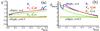Fig. 13 Effect of rBmin (the selection is defined by ⟨ B⟩ /Baxis > rBmin along the simulated crossing). The coefficient η,bmean is found by minimizing dist (Eq. (10)) for two force-free fields (lower curves: n = 0.5, upper curves: n = 1). Three probability distributions of P(b) are shown with different colors (for n = 0.5, the three curves are almost identical).

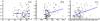Fig. 14 Correlations of the impact parameter p with a) the angle between the MC axis and the radial solar direction, b) the mean MC velocity (in km s-1), and c) the flux rope radius (in AU) found with the Lundquist fit. The straight line is a linear fit to the data points (MCs).

6. Application to subsets of MCs

6.1. Correlation between MC parameters

In this section, we explore the correlations between p and the other global parameters measured in the set of 100 MCs observed at 1 AU. In particular, we find unexpected correlations.

First, we examine the cone angle β, which is the angle between the MC axis to the solar radial direction. The number of detected MCs decreases with a lower β angle (Fig. 14a). Still, we find no correlation between β and p, showing that the crossing cases away from the MC nose (low β values) have no special biased impact parameter when the few cases corresponding to a leg crossing are filtered out (β > 30°). This justifies the use of models with a locally straight axis (e.g., Owens et al. 2012,and references therein).

As reported by Lepping & Wu (2010), we also find no significant correlation between p and B₀ (the deduced axial field strength). We agree with their interpretation that B_axis of MCs is expected to be spread in a large range (about a factor 10), so that the dispersion of B_axis is likely to mask any weak dependence B₀(p). Indeed, we find such dependence in the models. The dependance is weak for circular models (Fig. 4) and moderate for models with elongated cross sections. For example, with b = 2, B₀ monotonously decreases from 1 to ≈ 0.4 for an elliptical linear force-free field, while this decrease is much weaker, only down to ≈ 0.8, for an elliptical model with uniform current (not shown). Since we detected two indicators in favor of finding typical MCs between those models (ends of Sects. 3.3 and 4.2), B₀(p) is expected to have a relatively weak dependence (from 1 to ≈ 0.6) that can be easily masked by the large dispersion of B_axis in MCs.

Other global parameters are not or are only weakly correlated with p, except for two: V (mean velocity of the MC along the spacecraft trajectory) and R (flux rope radius deduced from the Lundquist field). The Pearson’s correlation coefficient is 0.26 and 0.35 for V and R respectively, and a linear fit also clearly shows the trends (Fig. 15b, c). The correlation V(p) is the most surprising since V is measured directly from the data and is a robust quantity (weakly dependent on the selected MC boundaries). Such a result could not be interpreted as a real velocity shear between the MC core and its surrounding since by its magnitude this effect would shear apart the flux rope before its arrival to 1 AU (the consequences of this particular behavior around 1 AU are neither observed and nor plausible). The strong correlation R(p) is also surprising. Still, we emphasize the study of V because R could be affected by the amount of reconnection achieved between the MC and the overtaken magnetic field as deduced by the presence of a back region in MCs (Dasso et al. 2006, 2007; Ruffenach et al. 2012).

Fig. 15 Properties of impact parameter distributions for different MC groups. a) Slope of the linear fit of when MCs are first ordered with a growing mean velocity V, then binned in groups of 16 cases (running grouping with increasing V). The three curves represent this slope, with the black line corresponding to the mean V of each group and the blue (resp. red) line corresponding to the minimum (resp. maximum) value of each group. The horizontal dashed line is the slope for all MCs (slope of the black line in Fig. 1). The horizontal axis is scaled with the logarithm of V. b), c) Probability distribution, , as in Fig. 1, with MCs separated in two groups according to their mean velocity V.

6.2. Sets of MCs with different aspect ratios

We investigate the above puzzling result by analyzing probability distributions, as in Fig. 1, but for MCs with a restricted interval of velocity. Due to the fairly low number of MCs, we are limited to a relatively coarse sampling in V.

The probability distributions are fitted by a straight line (such as the black line in Fig. 1) in order to decrease the statistical fluctuations inside the p bins and summarize the distribution information to the slope. For a histogram of N MCs that is distributed according to a linear function of p, the constrain that the sum of the probabilities is unity implies a relation between the slope of this distribution and the mean value of p, noted ⟨ p⟩, as $\mathrm{slope}\mathrm{=}\mathrm{12}\mathrm{\Delta }\mathit{p}\mathrm{(}\mathrm{⟨}\mathit{p}\mathrm{⟩}\mathrm{-}\mathrm{1}\mathit{/}\mathrm{2}\mathrm{)}\mathit{/}\mathrm{(}\mathrm{1}\mathrm{-}{\mathit{N}}^{-2}\mathrm{)}\mathit{,}$(15)with Δp being the bin size. For N slightly large (say N ≥ 10), Eq. (15) shows that the slope is almost independent of N and simply related to ⟨ p⟩. It implies that the slope is a relatively robust quantity, even for a low number N of MCs used to build the distribution. The expected statistical fluctuations on ⟨ p⟩ are of the order of $\mathrm{⟨}\mathit{p}\mathrm{⟩}\mathit{/}\sqrt{\mathit{N}}$, which translate to fluctuations of the slope $\mathrm{\approx }\mathrm{(}\mathrm{slope}\mathrm{+}\mathrm{6}\mathrm{\Delta }\mathit{p}\mathrm{)}\mathit{/}\sqrt{\mathit{N}}\mathrm{\approx }\mathrm{0.1}$ for a slope ≈ − 0.2 (Fig. 1), Δp = 0.1 and N = 16.

Next, we ordered the MC data according to growing values of V and computed the evolution of the slope for N MCs progressively shifting to higher V values. With N = 16, fluctuations of the slope are ≤0.1, as expected. There is a sudden change for V above ≈ 550 km s^-1 (Fig. 15a). A similar result is obtained for larger N values, with fewer fluctuations, but with a reduced dynamic (in both axis directions). Indeed, separating the MCs to two groups shows two different distribution functions (Fig. 15b, c). Similar results are found when the above ordering with V is replaced by one with R.

With the results of Sects. 5.2 and 5.4, we interpret this result as the presence of two main groups of MCs. The slower ones, V < 550 km s^-1, which are also the most numerous (84 MCs), have an oblate cross section with a mean aspect ratio between 2 and 3, depending the model used, similar to the full set of MCs. However, the faster MCs at 1 AU have a nearly flat distribution, so they are mostly round whatever model is selected (within the explored ones). It would be worth checking this conclusion with more MCs since this group is limited to 16 MCs. These MCs are also typically larger and have a stronger magnetic field since V has a correlation coefficient of 0.32 with R and 0.68 with B₀ (for the full set of 100 MCs). Indeed, a variation of the slope of with MCs ordered with R was found to be similar to that of V (Fig. 15a). This is not the case with B₀ since there is no significant correlation between B₀ and p (Sect. 6.1).

Why would faster and larger MCs typically have nearly round cross section? On first thought, a faster MC would imply a larger snowplow effect, plausibly generating a larger sheath that can compress the flux rope more, and thus induce a flatter cross section. However, the velocity is measured at 1 AU and the above result could mean that those faster MCs were on average less decelerated than others, so that the distortion from the surrounding solar wind was less important than for other MCs. Moreover, faster MCs spend less time from solar eruption to their arrival at the point where they are observed in situ, and the distortion mechanisms are expected to be less effective. Another plausibly complementary answer is that the faster MCs have typically a stronger magnetic field, so that the magnetic tension is stronger and keeps the cross section rounder.

7. Conclusions

The MCs observed at 1 AU are classically fitted with a Lundquist model (Lepping et al. 1990). In the set of 120 MCs analyzed, only 11% (13/120) of the MCs could not be satisfactorily fitted (either the flux rope handedness could not be determined or the fit did not converge), while 6% (7/120) of the MCs are crossed too far away from the nose to provide reliable fit results. For the remaining 100 MCs, the fit provides an estimation of the impact parameter (p). The observed probability distribution, , of these MCs is found to decrease strongly with p (Lepping & Wu 2010, and Fig. 1). Compared to an expected almost uniform distribution, this could imply that about half of the MCs are not detected by in situ observations. Is this decrease due to a strong selection effect, like on the magnetic field strength and/or the amount of field-rotation angle? Or are the MCs observed only in about one-third of ICMEs because more criteria are used to define ICMEs than MCs? Moreover, several of the less restrictive criteria used to identify ICMEs are expected to be independent of the impact parameters (such as temperature, composition, and ionization level). In order to answer these questions, we explored the parameter space of flux rope models with force-free fields. We simulated spacecraft crossings and performed a least-square fit of the synthetic data with a Lundquist field, using the same procedure as for observations of real MCs. The fit provided an estimated impact parameter p that we compared to the true one known from the synthetic model.

For models with circular cross sections, we found that selection effects with magnetic field strength and field-rotation angle are present only for large p values, so they cannot explain the gradual decrease of . This result is found for a broad variety of magnetic field profiles ranging from nearly uniform to peaked field strength across the flux rope.

Next, exploring non-circular cross sections, we found that the aspect ratio, b, of the cross section is the main parameter affecting the estimated impact parameter p. For flux ropes flatter in the propagating direction (corresponding to b > 1), p is more biased to lower values, compared to the true one, as b is increased. This effect implies simulated distributions , which are close to observed ones with b ≈ 2 for an elliptical model with uniform axial current density. For linear force-free fields with elliptical cross sections, p is less affected by b. However, the field strength decreases more rapidly away from the flux rope axis, so that the selection effect on the field strength enhances the dependence of on b.

We also explored other effects that can bias the probability distribution of p. We found that bending the cross section in a bean-like shape has a small effect on the estimated p. A much larger effect is present if the cross section is set broader than an ellipse at large distance from the axis. An extreme case is a rectangular cross section. In that case, the linear force-free model corresponds to an even more biased p than the above elliptical model with uniform axial current density, and b ≈ 1.5 is sufficient to reproduce the observed distribution . Finally, we found that for all the models explored, the rotation angle along the spacecraft trajectory is above 90°, except for large p values (at least p ≥ 0.7). Then, a selection effect on this parameter cannot explain . Furthermore, only a selection criterium around 40° can lead to a computed in agreement with for large p values. This is in agreement with the minimum rotation angle found in the set of MCs analyzed by Lepping & Wu (2010).

We conclude that the observed distribution is mainly shaped by the oblateness of the MC cross section, with some contribution by a field strength selection when the flux rope is close to a linear force-free field. Still, even in this last case, typically more than 70% of the flux ropes are expected to be detected. Even adding infrequent cases that are not detected because of very large perturbations (so that the field rotation is not detected), a crossing within a leg, or strongly interacting MCs, this implies a low amount of undetected flux rope, well below two thirds. So we conclude that a large majority of flux ropes can be expected to be detected. ICMEs could still have a flux rope without strictly fulfilling all MC criteria, such as a strong enough magnetic field strength or a low enough proton temperature. These cloud-like events are reported in Lepping et al. (2005). The non-MC ICMEs could also be events encountered outside the flux rope limits or such ICMEs would contain none.

We also get results beyond the initial questions. The main dependence of on the aspect ratio b allows a key property of the distribution P(b) for MCs to be constrained: the mean of the aspect ratio. With an elliptical model with uniform current density, sets the mean of b near 2.3, independently of the broadness of distribution. This last property is approximately kept for a linear-force field, but the mean of b is shifted to around 3 with a slight dependence on the amount of the selection effect of the field strength. Then, we conclude that the observed implies that MCs are moderately oblate at 1 AU, at least on average.

We further analyzed the observed MCs by separating them into groups with different physical parameters. In contrast to most MCs, the faster MCs (above ≈ 550 km s^-1) have a flat distribution. This implies that the faster MCs, which typically also have both larger radius and field strength, are nearly round, while the slower ones have typically the above mean oblateness. Finally, we found two results indicating that the typical magnetic field profile in MCs is between a linear force-free field and one with a constant axial current density:

• First, the mean field strength observed along the spacecrafttrajectory is systematically above what is predicted by a linearforce-free field, but below the prediction given by a constantcurrent model. This is independent of the aspect ratio of the crosssection, in agreement with a previous study (Gulisanoet al. 2005).

• Second, the distribution computed with a distribution of b, derived to fit , shows systematic biases, both at low and large p values, with the opposite tendency for both types of magnetic fields. This conclusion is also coherent with the flatter field strength profile found in MCs compared to a Lundquist field. Then, both the current distribution and the oblateness of the flux ropes contribute to a relatively flat profile of the field strength.

Acknowledgments

The authors thank the referee for carefully reading, and thus improving the manuscript and Noé Lugaz for useful comments. The authors acknowledge financial support from ECOS-Sud through its cooperative science program (N° A08U01). This work was partially supported by the Argentinean grants UBACyT 20020090100264, PIP 11220090100825/10 (CONICET), and PICT-2007-856 (ANPCyT). S.D. is member of the Carrera del Investigador Científico, CONICET. S.D. acknowledges support from the Abdus Salam International Centre for Theoretical Physics (ICTP), as provided in the frame of his regular associateship. The work of M.J. is funded by a contract from the AXA Research Fund.

References

All Tables

All Figures

Fig. 1 Probability distribution, , of the impact parameter (p). The results of MCs observed by WIND at 1 AU and fitted by the Lundquist model (Lepping & Wu 2010; Lepping et al. 1990) are shown with a histogram having 10 bins of p. Black curve: a linear fit to the histogram. Red curve: the Gaussian function derived by Lepping & Wu (2010). The histogram in the top panel has 100 MCs, while the one in the bottom panel is restricted to the 74 best observed MCs (quality 1, 2).

In the text

	Fig. 2 Drawing defining the geometry parameters for a spacecraft crossing an MC. The fit of the Lundquist field is schematized by the blue circle, while the black ellipse delimitates the half extension of the MC boundary. In this figure, we scale the drawing with the semi-minor axis of the ellipse set to unity. The true impact parameter, y/b, is larger than p.
In the text

Fig. 3 Examples of circular models (black dots) least square fitted with the Lundquist field (red curves). Three non-linear force-free models (n = 0.1,0.5,2) are selected to represent strong departure to the Lundquist field (n = 1). The true impact parameter, y/b, is either null (left) or large (right). Bz is the axial field component, and By is the azimuthal field component for y = 0. The field strength of the model on the axis, Baxis, is normalized to 1.

In the text

Fig. 4 a) Dependence of the true impact parameter, y/b, b) the fitted Lundquist field strength on the axis, B0, c) the normalized deviation, dev/ ⟨B⟩, and d) the mean field magnitude ⟨ B⟩ normalized to B0 in function of the impact parameter, p, found by fitting the Lundquist field to the models. The parameter n describes the profile of the axial component of the magnetic field and electric current, see Eqs. (4), (5).

In the text

	Fig. 5 Dependence of the rotation angle, ω, of the magnetic field component orthogonal to the axis in function of the impact parameter, p, found by fitting the Lundquist field to circular models (Eqs. (3), (4)). The dots are the results obtained by Lepping & Wu (2010) for 65 MCs (see their Fig. 3B).
In the text

Fig. 6 Drawing defining the regions of the parameter space explored. The red line indicates the circular models analyzed in Sect. 3. The MC boundary is elliptical for the blue region and is deformed to a bean shape in the green region. The two blue lines indicate the elliptical models analyzed in Sect. 4. Finally, the purple line indicates an extreme case where the MC boundary is rectangular. n defines the axial electric current and magnetic field component (Eqs. (3), (4)). A cross section elongated orthogonally to the spacecraft trajectory has b > 1 (Fig. 2).

In the text

	Fig. 7 Examples of two elliptical models (n = 0.5,1, black dots) least square fitted with the Lundquist field (red curves) for a large true impact parameter, y/b = 0.9. Bz is the axial field component, and By is the field component both orthogonal to the simulated trajectory and to the flux rope axis.
In the text

	Fig. 8 Dependence of the true impact parameter, y/b, and of the normalized deviation, dev/ ⟨B⟩ in function of the fitted impact parameter p, found by fitting the Lundquist field to elliptical boundary models. The parameter n describes the profile of the axial current (Eqs. (3), (4)).
In the text

	Fig. 9 Dependence of the rotation angle, ω, of the magnetic field component orthogonal to the axis in function of the impact parameter, p, found by fitting the Lundquist field to two models with an elliptical boundary a), b) and one with a rectangular boundary c). The dots are the results obtained by Lepping & Wu (2010) for 65 MCs (see their Fig. 3B).
In the text

	Fig. 10 Probability distribution of the impact parameter, , deduced from various models and a uniform probability distribution of y/b. The thin curves are without selection effect and the thick curves are for ⟨ B⟩ /Baxis > 0.25 and a magnetic field rotation angle greater than 90°. The dashed black curve is a Gaussian function fitted to observations (Fig. 1).
In the text

Fig. 11 Approximate dependence of the true impact parameter, y/b, in function of the estimated impact parameter, p, for bent cross sections derived from Démoulin & Dasso’s (2009) results (derived from rBx, see text in Sect. 4.5). The bending increases with the dimensionless parameter a. Linear force-free models (n = 1, Eq. (4)) are shown for two aspect ratio b. The black dashed line is the relation found by fitting the Lundquist field to the elliptic (a = 0) model with n = 1.

In the text

	Fig. 12 Probability distributions from Eq. (9) and P(b) from Eqs. (11), (13) for the minimum of dist(η,bmean) as defined by Eq. (10). of Fig. 1 is added in a), d). Two force-free elliptical models are shown: a)–c) n = 0.5 (constant current density), d)–f) n = 1 (linear force-free) for rBmin = 0.25 and ωmin = 0. The three P(b) functions, shown with three colors, imply similar results.
In the text

	Fig. 13 Effect of rBmin (the selection is defined by ⟨ B⟩ /Baxis > rBmin along the simulated crossing). The coefficient η,bmean is found by minimizing dist (Eq. (10)) for two force-free fields (lower curves: n = 0.5, upper curves: n = 1). Three probability distributions of P(b) are shown with different colors (for n = 0.5, the three curves are almost identical).
In the text

	Fig. 14 Correlations of the impact parameter p with a) the angle between the MC axis and the radial solar direction, b) the mean MC velocity (in km s-1), and c) the flux rope radius (in AU) found with the Lundquist fit. The straight line is a linear fit to the data points (MCs).
In the text

Fig. 15 Properties of impact parameter distributions for different MC groups. a) Slope of the linear fit of when MCs are first ordered with a growing mean velocity V, then binned in groups of 16 cases (running grouping with increasing V). The three curves represent this slope, with the black line corresponding to the mean V of each group and the blue (resp. red) line corresponding to the minimum (resp. maximum) value of each group. The horizontal dashed line is the slope for all MCs (slope of the black line in Fig. 1). The horizontal axis is scaled with the logarithm of V. b), c) Probability distribution, , as in Fig. 1, with MCs separated in two groups according to their mean velocity V.

In the text

References

- Antoniadou, I., Geranios, A., Vandas, M., et al. 2008, Planet. Space Sci., 56, 492 [NASA ADS] [CrossRef] [Google Scholar]
- Burlaga, L. F. 1988, J. Geophys. Res., 93, 7217 [NASA ADS] [CrossRef] [Google Scholar]
- Burlaga, L. F. 1995, Interplanetary magnetohydrodynamics (New York: Oxford University Press) [Google Scholar]
- Burlaga, L., Sittler, E., Mariani, F., & Schwenn, R. 1981, J. Geophys. Res., 86, 6673 [Google Scholar]
- Cane, H. V., & Richardson, I. G. 2003, J. Geophys. Res., 108, 1156 [Google Scholar]
- Cargill, P. J., & Schmidt, J. M. 2002,Ann. Geophys., 20, 879 [Google Scholar]
- Cid, C., Hidalgo, M. A., Nieves-Chinchilla, T., Sequeiros, J., & Viñas, A. F. 2002, Sol. Phys., 207, 187 [NASA ADS] [CrossRef] [Google Scholar]
- Dasso, S., Mandrini, C. H., Démoulin, P., & Farrugia, C. J. 2003, J. Geophys. Res., 108, 1362 [NASA ADS] [CrossRef] [Google Scholar]
- Dasso, S., Gulisano, A. M., Mandrini, C. H., & Démoulin, P. 2005a,Adv. Spa. Res., 35, 2172 [Google Scholar]
- Dasso, S., Mandrini, C. H., Démoulin, P., Luoni, M. L., & Gulisano, A. M. 2005b,Adv. Spa. Res., 35, 711 [Google Scholar]
- Dasso, S., Mandrini, C. H., Démoulin, P., & Luoni, M. L. 2006, A&A, 455, 349 [NASA ADS] [CrossRef] [EDP Sciences] [Google Scholar]
- Dasso, S., Nakwacki, M. S., Démoulin, P., & Mandrini, C. H. 2007, Sol. Phys., 244, 115 [NASA ADS] [CrossRef] [Google Scholar]
- Dasso, S., Mandrini, C. H., Schmieder, B., et al. 2009, J. Geophys. Res., 114, A02109 [NASA ADS] [CrossRef] [Google Scholar]
- Démoulin, P., & Dasso, S. 2009, A&A, 507, 969 [NASA ADS] [CrossRef] [EDP Sciences] [Google Scholar]
- Farrugia, C. J., Janoo, L. A., Torbert, R. B., et al. 1999, in Solar Wind Nine, eds. Habbal, S. R., Esser, R., Hollweg, J. V., & Isenberg, P. A., AIP Conf. Proc., 471, 745 [Google Scholar]
- Farrugia, C. J., Berdichevsky, D. B., Möstl, C., et al. 2011,J. Atmos. Sol. Terr. Phys., 73, 1254 [Google Scholar]
- Goldstein, H. 1983, in Solar Wind Five, NASA CP-2280, ed. M. Neugebauer, 731 [Google Scholar]
- Gosling, J. T. 1990, in Physics of magnetic flux ropes (A92-31201 12-75) (Washington, DC: American Geophysical Union), 58, 343 [Google Scholar]
- Gulisano, A. M., Dasso, S., Mandrini, C. H., & Démoulin, P. 2005,J. Atmos. Sol. Terr. Phys., 67, 1761 [Google Scholar]
- Gulisano, A. M., Dasso, S., Mandrini, C. H., & Démoulin, P. 2007,Adv. Spa. Res., 40, 1881 [Google Scholar]
- Harrison, R. A., Davies, J. A., Rouillard, A. P., et al. 2009, Sol. Phys., 256, 219 [NASA ADS] [CrossRef] [Google Scholar]
- Hidalgo, M. A. 2011, J. Geophys. Res., 116, 2101 [CrossRef] [Google Scholar]
- Hidalgo, M. A., Cid, C., Vinas, A. F., & Sequeiros, J. 2002, J. Geophys. Res., 107, 1002 [CrossRef] [Google Scholar]
- Howard, T. A. 2011,J. Atmos. Sol. Terr. Phys., 73, 1242 [Google Scholar]
- Hu, Q., & Sonnerup, B. U. Ö. 2002, J. Geophys. Res., 107, 1142 [CrossRef] [Google Scholar]
- Hu, Q., Smith, C. W., Ness, N. F., & Skoug, R. M. 2005, J. Geophys. Res., 110, A09S03 [CrossRef] [Google Scholar]
- Isavnin, A., Kilpua, E. K. J., & Koskinen, H. E. J. 2011, Sol. Phys., 273, 205 [NASA ADS] [CrossRef] [Google Scholar]
- Jian, L., Russell, C. T., Luhmann, J. G., & Skoug, R. M. 2006, Sol. Phys., 239, 393 [NASA ADS] [CrossRef] [Google Scholar]
- Kilpua, E. K. J., Liewer, P. C., Farrugia, C., et al. 2009, Sol. Phys., 254, 325 [NASA ADS] [CrossRef] [Google Scholar]
- Kilpua, E. K. J., Jian, L. K., Li, Y., Luhmann, J. G., & Russell, C. T. 2011,J. Atmos. Sol. Terr. Phys., 73, 1228 [Google Scholar]
- Kilpua, E. K. J., Jian, L. K., Li, Y., Luhmann, J. G., & Russell, C. T. 2012, Sol. Phys., 56 [Google Scholar]
- Leitner, M., Farrugia, C. J., Möstl, C., et al. 2007, J. Geophys. Res., 112, A06113 [NASA ADS] [CrossRef] [Google Scholar]
- Lepping, R. P., & Wu, C. C. 2010,Ann. Geophys., 28, 1539 [Google Scholar]
- Lepping, R. P., Burlaga, L. F., & Jones, J. A. 1990, J. Geophys. Res., 95, 11957 [NASA ADS] [CrossRef] [Google Scholar]
- Lepping, R. P., Berdichevsky, D. B., & Ferguson, T. J. 2003, J. Geophys. Res., 108, 1356 [CrossRef] [Google Scholar]
- Lepping, R. P., Wu, C.-C., & Berdichevsky, D. B. 2005, Ann. Geophys., 23, 2687 [NASA ADS] [CrossRef] [Google Scholar]
- Lepping, R. P., Berdichevsky, D. B., Wu, C. C., et al. 2006, Ann. Geophys., 24, 215 [NASA ADS] [CrossRef] [Google Scholar]
- Lepping, R. P., Narock, T. W., & Chen, H. 2007, Ann. Geophys., 25, 2641 [NASA ADS] [CrossRef] [Google Scholar]
- Liu, Y., Luhmann, J. G., Huttunen, K. E. J., et al. 2008, ApJ, 677, L133 [NASA ADS] [CrossRef] [Google Scholar]
- Lugaz, N., & Roussev, I. 2011,J. Atmos. Sol. Terr. Phys., 73, 1187 [Google Scholar]
- Lugaz, N., Manchester, IV, W. B., & Gombosi, T. I. 2005a, ApJ, 634, 651 [Google Scholar]
- Lugaz, N., Manchester, IV, W. B., & Gombosi, T. I. 2005b, ApJ, 627, 1019 [Google Scholar]
- Lugaz, N., Kintner, P., Möstl, C., et al. 2012, Sol. Phys., 279, 497 [NASA ADS] [CrossRef] [Google Scholar]
- Lundquist, S. 1950, Ark. Fys., 2, 361 [Google Scholar]
- Lynch, B. J., Zurbuchen, T. H., Fisk, L. A., & Antiochos, S. K. 2003, J. Geophys. Res., 108, A01239 [NASA ADS] [CrossRef] [Google Scholar]
- Manchester, W. B. I., Gombosi, T. I., Roussev, I., et al. 2004, J. Geophys. Res., 109, A02107 [Google Scholar]
- Marubashi, K. 1997, in Coronal Mass Ejections, Geophys. Monogr., 99, 147 [CrossRef] [Google Scholar]
- Marubashi, K., & Lepping, R. P. 2007,Ann. Geophys., 25, 2453 [Google Scholar]
- Marubashi, K., Cho, K.-S., Kim, Y.-H., Park, Y.-D., & Park, S.-H. 2012, J. Geophys. Res., 117, 1101 [Google Scholar]
- Möstl, C., Farrugia, C. J., Biernat, H. K., et al. 2009a, Sol. Phys., 256, 427 [NASA ADS] [CrossRef] [Google Scholar]
- Möstl, C., Farrugia, C. J., Miklenic, C., et al. 2009b, J. Geophys. Res., 114, A04102 [NASA ADS] [CrossRef] [Google Scholar]
- Mulligan, T., Russell, C. T., Anderson, B. J., et al. 1999, J. Geophys. Res., 104, 28217 [NASA ADS] [CrossRef] [Google Scholar]
- Odstrcil, D., Riley, P., & Zhao, X. P. 2004, J. Geophys. Res., 109, 2116 [Google Scholar]
- Owens, M. J., Démoulin, P., Savani, N. P., Lavraud, B., & Ruffenach, A. 2012, Sol. Phys., 278, 435 [NASA ADS] [CrossRef] [Google Scholar]
- Press, W. H., Teukolsky, S. A., Vetterling, W. T., & Flannery, B. P. 1992, Numerical Recipes (Cambridge University Press) [Google Scholar]
- Richardson, I. G., & Cane, H. V. 2004, J. Geophys. Res., 109, A09104 [Google Scholar]
- Richardson, I. G., & Cane, H. V. 2010, Sol. Phys., 264, 189 [NASA ADS] [CrossRef] [Google Scholar]
- Riley, P., Linker, J. A., Mikić, Z., et al. 2003, J. Geophys. Res., 108, 1272 [CrossRef] [Google Scholar]
- Romashets, E. P., & Vandas, M. 2003, Geophys. Res. Lett., 30, 2065 [Google Scholar]
- Romashets, E., & Vandas, M. 2009, A&A, 499, 17 [NASA ADS] [CrossRef] [EDP Sciences] [Google Scholar]
- Rouillard, A. P. 2011,J. Atmos. Sol. Terr. Phys., 73, 1201 [Google Scholar]
- Ruffenach, A., Lavraud, B., Owens, M. J., et al. 2012, J. Geophys. Res., 117, A09101 [NASA ADS] [CrossRef] [Google Scholar]
- Savani, N. P., Rouillard, A. P., Davies, J. A., et al. 2009,Ann. Geophys., 27, 4349 [Google Scholar]
- Savani, N. P., Owens, M. J., Rouillard, A. P., Forsyth, R. J., & Davies, J. A. 2010, ApJ, 714, L128 [Google Scholar]
- Sonnerup, B. U. Ö., Hasegawa, H., Teh, W.-L., & Hau, L.-N. 2006, J. Geophys. Res., 111, 9204 [CrossRef] [Google Scholar]
- Vandas, M., & Romashets, E. P. 2003, A&A, 398, 801 [NASA ADS] [CrossRef] [EDP Sciences] [Google Scholar]
- Vandas, M., Odstrčil, D., & Watari, S. 2002, J. Geophys. Res., 107, 1236 [Google Scholar]
- Vandas, M., Romashets, E., & Watari, S. 2005, Planet. Space Sci., 53, 19 [NASA ADS] [CrossRef] [Google Scholar]
- Vandas, M., Romashets, E., & Geranios, A. 2010,Ann. Geophys., 28, 1581 [Google Scholar]
- Wang, Y. M., Ye, P. Z., & Wang, S. 2003, J. Geophys. Res., 108, 1370 [CrossRef] [Google Scholar]
- Wimmer-Schweingruber, R. F., Crooker, N. U., Balogh, A., & et al. 2006, Space Sci. Rev., 123, 177 [NASA ADS] [CrossRef] [Google Scholar]
- Wood, B. E., Rouillard, A. P., Möstl, C., et al. 2012, Sol. Phys., 281, 369 [NASA ADS] [Google Scholar]
- Wu, C.-C., & Lepping, R. P. 2011, Sol. Phys., 269, 141 [NASA ADS] [CrossRef] [Google Scholar]
- Xiong, M., Zheng, H., Wang, Y., & Wang, S. 2006, J. Geophys. Res., 111, A08105 [NASA ADS] [CrossRef] [Google Scholar]
- Zurbuchen, T. H., & Richardson, I. G. 2006, Space Sci. Rev., 123, 31 [NASA ADS] [CrossRef] [Google Scholar]