| Issue |
A&A
Volume 550, February 2013
|
|
|---|---|---|
| Article Number | A117 | |
| Number of page(s) | 9 | |
| Section | Interstellar and circumstellar matter | |
| DOI | https://doi.org/10.1051/0004-6361/201220212 | |
| Published online | 05 February 2013 | |
Molecular clumps and star formation associated with the infrared dust bubble N131
1
National Astronomical Observatories, Chinese Academy of
Sciences,
100012
Beijing
PR China
e-mail: This email address is being protected from spambots. You need JavaScript enabled to view it.
2
NAOC – TU Joint Center for Astrophysics, 850000
Lhasa, PR
China
3
University of the Chinese Academy of Sciences,
100080
Beijing, PR
China
Received:
13
August
2012
Accepted:
19
December
2012
Abstract
Aims. The aim is to explore the interstellar medium around the dust bubble N131 and search for signatures of star formation.
Methods. We have performed a multiwavelength study around the N131 with data taken from large-scale surveys of infrared observation with online archive. We present new observations of three CO J = 1−0 isotope variants from Purple Mountain Observatory 13.7 m telescope. We analyzed the distribution of the molecular gas and dust in the environment of the N131. We used color−color diagrams to search for young stellar objects and to identify ionizing star candidates.
Results. The kinematic distance of ~8.6 kpc has been adopted as the distance of the bubble N131 from the Sun in this work. We find a ring of clouds in CO emission coincident with the shell of N131 seen in the Spitzer telescope images, and two giant elongated molecular clouds of CO emission appearing on opposite sides of the ringlike shell of N131. There is a cavity within the bubble at 1.4 GHz and 24 μm. Seven IRAS point sources are distributed along the ringlike shell of the bubble N131. Fifteen ionizing stars and 63 YSO candidates have been found. The clustered class I and II YSOs are distributed along the elongated clouds in the line of sight.
Key words: infrared: ISM / stars: formation / ISM: bubbles / HII regions
© ESO, 2013
1. Introduction
Churchwell et al. (2006, 2007) have detected and cataloged about 600 midinfrared dust (MIR) bubbles between longitudes −60° and +60°. The IR dust bubbles may be produced by ionizing O- and/or B-type stars, which are located inside the bubble. The ultraviolet (UV) radiation from ionizing stars may heat dust and ionize the gas to form an expanding bubble shell (Watson et al. 2008). Simpson et al. (2012) present a new catalog of 5106 infrared bubbles created through visual classification via the online citizen science website “The Milky Way Project”1, which provides a crowd-sourced map of bubbles and arcs in the Milky Way, and will enable better statistical analysis of Galactic star-forming sites. Beaumont & Williams (2010) report CO J = 3−2 maps of 43 Spitzer identified bubbles, which suggests that expanding shock fronts are poorly bound by molecular gas and that cloud compression by these shocks may be limited. Watson et al. (2008) present an analysis of wind-blown, parsec-sized, midinfrared bubbles, and associated star formation, and suggest that more than a quarter of the bubbles may have triggered the formation of massive objects.
A few individual bubbles have been studied well, such as N22 (Ji et al. 2012), N49 (Watson et al. 2008; Deharveng et al. 2010; Zavagno et al. 2010), N65 (Petriella et al. 2010), N68 (Zhang & Wang 2012b), and S51 (Zhang & Wang 2012a). There are many models and observations to explain the dusty wind-blown bubbles, such as bubble N49 of Everett & Churchwell (2010). Recently, we have reported an expanding ringlike shell of the bubble S51, which shows a rare front side located within the shell in the line of sight, by employing 13CO and C18O J = 1−0 emission lines of the Mopra Telescope (Zhang & Wang 2012a). We also investigated the star formation around the bubble N68, which suggests that the massive star formation at the ringlike shell is very active (Zhang & Wang 2012b).
Toward the bubble N131, in this work, we carried out new observations of the J = 1−0 transitions of 12CO, 13CO, and C18O using the telescope of the Purple Mountain Observatory (PMO) at Qinghai province in China. we mainly report several molecular clumps associated well with the IR dust bubble N131. We also aim to explore its surrounding ISM and search for star formation spots. We describe the data in Sect. 2; the results and discussion are presented in Sect. 3; Sect. 4 summarizes the results.
2. Observation and data processing
2.1. The online archive
The data of the online archive used in this work include GLIMPSE (Benjamin et al. 2003; Churchwell et al. 2009), MIPSGAL (Carey et al. 2009), the Two Micron All Sky Survey (2MASS)2 (Skrutskie et al. 2006), IRAS (Neugebauer et al. 1984), and NVSS (Condon et al. 1998). GLIMPSE is an MIR survey of the inner Galaxy performed with the Spitzer Space Telescope. We used the mosaicked images from GLIMPSE and the GLIMPSE Point-Source Catalog (GPSC) in the Spitzer-IRAC (3.6, 4.5, 5.8, and 8.0 μm). IRAC has an angular resolution between 1.5′′ and 1.9′′ (Fazio et al. 2004; Werner et al. 2004). MIPSGAL is a survey of the same region as GLIMPSE, using the MIPS instrument (24 and 70 μm) on Spitzer. The MIPSGAL resolution is 6′′ at 24 μm. The IRAS Point Source Catalog consists of 245 889 sources found and verified by the IRAS (InfraRed Astronomy Satellite) at 12, 25, 60, and 100 μm. The NRAO VLA Sky Survey (NVSS) is a 1.4 GHz continuum survey covering the entire sky north of −40° declination (Condon et al. 1998); the NVSS survey has a noise of about 0.45 mJy beam-1.
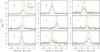 |
Fig. 1 12CO (red line), 13CO (black line), and C18O (green line) spectra at the peaks of the molecular clumps from A to I. The brightness temperature of each 13CO spectrum is multiplied by 2. |
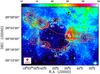 |
Fig. 2 Integrated intensity contours of the 12CO emission clouds superimposed on the GLIMPSE 8.0 μm colorscale. The contour levels range from 5.35 to 32.11 by 2.68 K km s-1. The integration range is from −14.5 to −6.5 km s-1. The letters from A to I indicate the positions of nine molecular clumps, and the area of each clump is indicated with dashed ellipse and polygon. The black symbols “■” indicate the positions of IRAS point sources. The white ellipse indicates the position of bubble N131, and the straight lines indicate the position of position-velocity diagram in Fig. 5. The beam size of 12CO emission is given in the filled red circle. The unit of the color bar is in MJy sr-1. |
2.2. The CO data of Purple Mountain Observatory
Our CO observations were made during May 2012 using the 13.7-m millimeter telescope of Qinghai Station at the Purple Mountain Observatory at Delingha3. We used the nine-pixel array receiver separated by ~180′′. The receiver was operated in the sideband separation of single sideband mode, which allows for simultaneous observations of three CO J = 1−0 isotope variants, with 12CO in the upper sideband (USB) and 13CO and C18O in the lower sideband (LSB). The half-power beam width (HPBW) is 52′′ ± 3′′, and the main beam efficiency is ~50% at ~110 GHz. The pointing and tracking accuracies are better than 5′′. The typical system temperature during our runs was around 110 K and varies by about 10% for each beam. A fast Fourier transform (FFT) spectrometer was used as the back end with a total bandwidth of 1 GHz and 16 384 channels. The velocity resolution is about 0.16 km s-1 at ~110 GHz.
On-the-fly (OTF) observing mode was applied for mapping observations. The antenna
continuously scanned a region of 20′ × 20′ centered on RA(J2000) =
19h52m09 61, Dec(J2000) =
26°22′13
61, Dec(J2000) =
26°22′13 4 with a scan
speed of 20″ s-1. The OFF position was chosen at RA(J2000) =
19h47m2400, Dec(J2000) =
28°29′240, where there
is extremely weak CO emission based on the CO survey of the Milky Way (Dame et al. 1987, 2001). The rms noise level was 0.2 K in main beam antenna temperature
4 with a scan
speed of 20″ s-1. The OFF position was chosen at RA(J2000) =
19h47m2400, Dec(J2000) =
28°29′240, where there
is extremely weak CO emission based on the CO survey of the Milky Way (Dame et al. 1987, 2001). The rms noise level was 0.2 K in main beam antenna temperature
 for 12CO (1−0), and 0.1 K for 13CO (1−0) and C18O
(1−0). The OTF data were then converted to 3-D cube data with a grid spacing of 30″. The
IRAM software package GILDAS4 and the software
package MIRIAD5 were used for the data reduction.
for 12CO (1−0), and 0.1 K for 13CO (1−0) and C18O
(1−0). The OTF data were then converted to 3-D cube data with a grid spacing of 30″. The
IRAM software package GILDAS4 and the software
package MIRIAD5 were used for the data reduction.
3. Analysis and the results
3.1. The dimension and distance of the bubble N131
We selected the IR dust bubble N131 from the catalog of Churchwell et al. (2006). They suggest that the N131 is a complete (closed ring)
IR dust bubble centered on l∗ = 63.084,
b∗ = −0.395, with an inner short radius
 , an inner long radius
 , and an eccentricity
of the ellipse
, and an eccentricity
of the ellipse  . By comparing the IR emission
with the integrated intensity of CO emission, the dimensions about the ring of cloud are
respectively rin = 5.20′,
Rin = 6.00′, and
eN131 = 0.50 centered on l = 63.095,
b = −0.404, or RA(J2000) =
19h52m215, Dec(J2000) =
+26°21′240. Here,
rin and Rin are the semiminor
and semimajor axes of the inner ellipse, respectively. By analyzing H2CO
absorption (VH2CO = 22.6 ± 0.1 km s-1)
against the UC HII region continuum emission
(VH110α = −9.3 ± 2.3 km s-1),
Watson et al. (2003) resolved the distance
ambiguity toward G63.05-0.34, which lies on the “far” kinematic distance
. By comparing the IR emission
with the integrated intensity of CO emission, the dimensions about the ring of cloud are
respectively rin = 5.20′,
Rin = 6.00′, and
eN131 = 0.50 centered on l = 63.095,
b = −0.404, or RA(J2000) =
19h52m215, Dec(J2000) =
+26°21′240. Here,
rin and Rin are the semiminor
and semimajor axes of the inner ellipse, respectively. By analyzing H2CO
absorption (VH2CO = 22.6 ± 0.1 km s-1)
against the UC HII region continuum emission
(VH110α = −9.3 ± 2.3 km s-1),
Watson et al. (2003) resolved the distance
ambiguity toward G63.05-0.34, which lies on the “far” kinematic distance
 kpc.
In fact, there is no distance ambiguity toward N131, because the derived “near” kinematic
distance is negative. The G63.05-0.34 is located at the position of the IRAS 19499+2613,
which is correlated with CO molecular clump A
(VCO = ~− 10.5 km s-1) in this work. Watson et al. (2010), however, adopted the velocity of
H2CO (~22.6 km s-1) in Watson
et al. (2003) to obtain a kinematic distance of ~2.4 kpc toward the bubble
N131. Actually, there is another CO velocity component at ~25.0 km s-1, which
is consistent with H2CO velocity at ~22.6 km s-1, but not
correlated with the ringlike shell of this bubble. This velocity component of
~22.6 km s-1 may belong to the foreground of the bubble N131. Therefore, we
adopt the kinematic distance DN131 = 8.6 kpc as the distance
of the bubble N131. The dimensions of the inner short radius and the inner long radius are
Drin = 13.0 pc
and DRin = 15.0 pc,
respectively.
kpc.
In fact, there is no distance ambiguity toward N131, because the derived “near” kinematic
distance is negative. The G63.05-0.34 is located at the position of the IRAS 19499+2613,
which is correlated with CO molecular clump A
(VCO = ~− 10.5 km s-1) in this work. Watson et al. (2010), however, adopted the velocity of
H2CO (~22.6 km s-1) in Watson
et al. (2003) to obtain a kinematic distance of ~2.4 kpc toward the bubble
N131. Actually, there is another CO velocity component at ~25.0 km s-1, which
is consistent with H2CO velocity at ~22.6 km s-1, but not
correlated with the ringlike shell of this bubble. This velocity component of
~22.6 km s-1 may belong to the foreground of the bubble N131. Therefore, we
adopt the kinematic distance DN131 = 8.6 kpc as the distance
of the bubble N131. The dimensions of the inner short radius and the inner long radius are
Drin = 13.0 pc
and DRin = 15.0 pc,
respectively.
3.2. Parameters of the spectra and molecular clumps
Figure 1 shows several spectra for 12CO,
13CO, and C18O at the peak locations of nine molecular clumps from
A to I (indicated in Fig. 2) defined on the basis of
13CO contours. For the nine molecular clumps, we detected strong
12CO and 13CO emission lines. At any position toward the N131,
however, we did not detect any C18O emission signal of more
than 3σ. We reported spectral information of the nine molecular clumps
in Table 1, and some derived parameters of the
molecular clumps in Table 2. In Table 1, Col. (1) lists the molecular clump name;
Cols. (2), (3) list the equatorial coordinates; Cols. (4)−(9) list the LSR velocity
VCO, the full width at half maximum (FWHM)
ΔVCO, and the peak brightness temperature
TCO of each clump using Gaussian fitting for CO emission
line. In Table 2, Cols. (1)−(4) show the name,
the dimension, and the integration temperature of each molecular clump, where the area of
each clump is indicated with a dashed ellipse and polygon in Fig. 2; Cols. (5)−(8) show the maximum and mean value of the ionizing
temperature and the H2 column density; Cols. (9)−(10) show the mass and
density of each molecular clump. Here, we assumed each molecular clump is under the local
thermal equilibrium (LTE) assumption, and used the theory of the radiation transfer and
molecular excitation (Winnewisser et al. 1979;
Garden et al. 1991). The excitation temperature
Tex and column density
 can
be calculated directly, assuming 12CO emission to be optically thick and the
beam-filling factor to be unity. The column densities of H2 were obtained by
adopting typical abundance ratios [H2]/[12CO] = 104 and
[12CO]/[13CO] = 60 in the ISM.
can
be calculated directly, assuming 12CO emission to be optically thick and the
beam-filling factor to be unity. The column densities of H2 were obtained by
adopting typical abundance ratios [H2]/[12CO] = 104 and
[12CO]/[13CO] = 60 in the ISM.
3.3. The ringlike shell
In Fig. 2, the 8.0 μm emission colorscale outlines clearly the distribution of molecular filament and clumpy structure toward the bubble N131. The 8.0 μm emission originates mainly in the polycyclic aromatic hydrocarbons (PAHs). Inside the N131, the 8.0 μm emission is much weaker than that at the ringlike shell. It is likely that the stellar wind from O- and/or early B-type stars have blown the PAHs onto the ringlike shell. In Fig. 3, the colorscale is the MIPSGAL 24 μm emission. Generally, there should be strong 24 μm emission and 1.4 GHz continuum emission inside bubble, such as in the dust bubbles S51 (Zhang & Wang 2012a) and N68 (Zhang & Wang 2012b). However, having nearly the same distribution as 8.0 μm emission, the 24 μm emission is very weak inside the bubble N131.
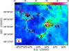 |
Fig. 3 Integrated intensity contours of the 13CO emission clouds superimposed on the MIPSGAL 24 μm colorscale. The contour levels range from 2.17 to 8.68 by 1.09 K km s-1. The integration range is from −14.5 to −6.5 km s-1. The letters from A to I indicate the positions of nine molecular clumps, and the symbols “”, “ × ”, and “■” indicate the positions of class I, class II, and IRAS point sources, respectively. The white ellipse indicates the position of bubble N131. The beam size of 12CO emission is given in the filled red circle. The unit of the color bar is in MJy sr-1. |
Parameters of the nine spectra.
Derived parameters of the CO molecular clumps.
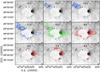 |
Fig. 4 Integrated intensity contours of the 12CO emission clouds every 1.0 km s-1 superimposed on the GLIMPSE 8.0 μm grayscale. The lowest contour level for each velocity panel from −14.5 to −6.5 km s-1 is 1.59, 1.37, 1.80, 2.24, 1.96, 2.19, 2.80, 1.22, and 0.95 K km s-1, respectively; the level increment of each panel is equal to the corresponding value of the lowest contour level. The blue, green, and red contours indicate the blueshifted, systematic, and redshifted velocities, respectively. The white ellipse indicates the position of bubble N131. |
Comparing 12CO emission in Fig. 2 with 13CO emission in Fig. 3, we can find that several molecular clumps were connected together to form the ringlike shell of the N131. The inner edge of the ringlike shell has a much sharper gradient of 12CO emission than the outer edge. Based on the distribution of optically thin 13CO in Fig. 3, we also found seven clumps A, B, E, F, ..., and I along the ringlike shell. The parameters of the clumps in Table 2 show that the dense cores of star formation may be forming in clumps. Therefore, the ringlike shell is a possible birth place of star formation that was triggered by the bubble N131.
3.4. Two elongated molecular clouds
In Fig. 2, we also found there are two giant elongated molecular clouds (AD and BC) of CO emission appearing on opposite sides of the ringlike shell of N131. Morphologically, each cloud is in alignment, and the central axis of each cloud nearly goes through the center of the N131. The densest position of each cloud is located at the ringlike shell of the N131, and the two clouds AD and BC have extensive structure outwardly. On the north and south of the clump A located at the ringlike shell, there also is an expanding tendency in the western direction. This morphology may be caused by the stellar wind within the bubble, but the possibility needs to be explored further.
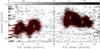 |
Fig. 5 Position-velocity diagram of the 12CO emission clouds along the white
straight lines in Fig. 2. The position
corresponding to offset 0 is at RA(J2000) =
19h52m17 |
Using the channel map (Fig. 4) of 12CO emission to investigate the velocity component of the bubble N131, The green contours in the panel of Fig. 4 show that the systematic velocity of the bubble is about −10.5 ± 0.5 km s-1, which is consistent with the velocity of the ionized gas (VH110α = −9.3 ± 2.3 km s-1, Watson et al. 2003). The velocity range of the cloud AD is from −9.5 to −6.5 km s-1 indicated with red contours, while the velocity of the cloud BC is from −14.5 to −11.5 km s-1 indicated with blue contours. We argue that the clouds AD and BC are, respectively, redshifted and blueshifted relative to the ringlike shell of the bubble.
In addition, along the central axis of the clouds AD and BC in Fig. 2, we made a position-velocity diagram in Fig. 5. Both the velocity gradient and velocity dispersion gradient are obvious from clumps A (B) to D (C). The velocity of the clump A on the ringlike shell is higher than that of the clump D, which is consistent with the redshifted velocity distribution of the bubble N68 (Zhang & Wang 2012b). For the cloud BC, the position-velocity diagram shows that clumps B and C may be two independent components. However, it is also possible that the molecular clumps B and C may be interacting. Figure 6 shows integrated intensity contours of the 12CO emission of the blueshifted (from −14.5 to −11.5 km s-1) and redshifted (from −9.5 to −6.5 km s-1) clouds. There is almost no overlap region between the blue- and redshifted clouds.
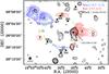 |
Fig. 6 Integrated intensity contours of the 12CO emission of the blueshifted and redshifted clouds superimposed on the 1.4 GHz NVSS continuum emission contours. The contour levels range from 3.20 to 19.20 by 1.60 K for the blueshifted cloud, and from 3.86 to 23.17 by 1.93 K for the redshifted cloud. The integration range is from −14.5 to −11.5 km s-1 for blueshifted cloud, and from −9.5 to −6.5 km s-1 for redshifted cloud. The contour levels of the 1.4 GHz NVSS continuum emission are 0.95, 1.26, 1.58, 3.16, 6.32, 12.64, 25.29, and 50.58 mJy beam-1. G63.049-0.348 is an HII region. The letters from A to I indicate the positions of nine molecular clumps, and the symbols “■” indicate the positions of IRAS point sources. The green ellipse indicates the position of bubble N131. The beam size of 12CO emission is given in the filled black circle. |
IRAS point sources around the bubble N131.
3.5. Lyman continuum flux
Figure 6 shows the 1.4 GHz NVSS continuum emission contours. The region of the continuum flux value above 2σ noise (or >0.9 mJy beam-1) was only integrated to consider as the reliable HII region candidates. From Fig. 6, it can be seen that there is no radio continuum emission within N131, except for a clump projected on the plane of the sky towards the center of the bubble. This fact, along with that the 24 μm emission being very weak inside the bubble, would indicate that hot dust and ionized gas have been evacuated by stellar wind (Watson et al. 2009). We also found that IR2 is located at the peak of HII region G63.049-0.348 (Gregory et al. 1996), suggesting that the IR2 (IRAS 19499+2613) may be the ionizing star of the HII region.
Assuming that the only radio feature in the center of N131 is associated with the bubble,
we derive the radio flux density of the HII region in about 0.016 Jy. The flux was
estimated by integrating each pixel for the signals of more than 2σ noise
from the NVSS fit image. This value should be taken with caution because the NVSS survey
has not added the flux contribution from large-scale structures. The number of stellar
Lyman photon, absorbed by the gas in the HII region, follows the relation Eq. (1) in Mezger
et al. (1974)![Mathematical equation: \begin{equation} \label{eq:nlcy} \left[\frac{N_{\rm Lyc}}{\rm s^{-1}}\right] \!= \!4.761\! \times\! 10^{48} a\left(\nu, T_{\rm e}\right)^{-1} \left[\frac{\nu}{\rm GHz}\right]^{0.1} \left[\frac{T_{\rm e}}{\rm K}\right]^{-0.45} \left[\frac{ S_{\nu}}{\rm Jy}\right] \left[\frac{D}{\rm kpc}\right]^2\!, \end{equation}](/articles/aa/full_html/2013/02/aa20212-12/aa20212-12-eq91.png) (1)where
a(ν,Te) is a slowly
varying function tabulated by Mezger & Henderson
(1967), for effective temperature of ionizing
star Te ~ 33 000 K and at radio wavelengths,
a(ν,Te) ~ 1. Finally, we
obtained Lyman continuum ionizing photons flux
log NLyc ~ 46.73 from nebula. Assuming the ionizing stars
belong to the O9.5 star with log NLyc ~ 47.84 (Panagia 1973), and the estimated
NLyc is a factor of 2 lower than the expected ionizing
photon flux from these stars (Beaumont & Williams
2010), it is suggested that there should be about 0.16 ionizing star of O9.5 star
to ionize the ISM within the bubble N131.
(1)where
a(ν,Te) is a slowly
varying function tabulated by Mezger & Henderson
(1967), for effective temperature of ionizing
star Te ~ 33 000 K and at radio wavelengths,
a(ν,Te) ~ 1. Finally, we
obtained Lyman continuum ionizing photons flux
log NLyc ~ 46.73 from nebula. Assuming the ionizing stars
belong to the O9.5 star with log NLyc ~ 47.84 (Panagia 1973), and the estimated
NLyc is a factor of 2 lower than the expected ionizing
photon flux from these stars (Beaumont & Williams
2010), it is suggested that there should be about 0.16 ionizing star of O9.5 star
to ionize the ISM within the bubble N131.
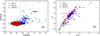 |
Fig. 7 a) GLIMPSE CC diagram [5.8]−[8.0] versus [3.6]−[4.5] for sources within a circle of about 10′ in radius centered on N131. The classification of class I, II, and III indicates different stellar evolutionary stages as defined by Allen et al. (2004). b) 2MASS CC diagram (H − Ks) versus (J − H). The sources for classes I and II are these, detected simultaneously by J, H, Ks, 3.6, 4.5, 5.8, and 8.0 μ bands; the sources for class III are located within a circle of 2.60′ (0.5 × rin) in a radius centered on N131. The gray squares represent the location of the main sequence and the giant stars (Bessell & Brett 1988). The parallel dotted lines are reddening vectors. The adopted interstellar reddening law is AJ / AV = 0.282, AH / AV = 0.175, and AKs / AV = 0.112 (Rieke & Lebofsky 1985), and the intrinsic colors (H − Ks)0 and (J − H)0 are obtained from Martins & Plez (2006). |
We also used the Effelsberg radio continuum data from the Galactic plane survey at 2695 MHz (only source component) to derive the Lyman continuum flux(Furst et al. 1990). The beam size of this survey is about 4.3′, rms is 20 mK in brightness temperature, and TB / S = 2.51 ± 0.05 [K/Jy]. Within a circle of 2.60′ (0.5 × rin) in radius centered on N131, the average brightness temperature is about 0.3 K, so the intensity is about 0.120 Jy. Using Eq. (1), we obtained the Lyman continuum flux log NLyc ~ 47.63. After considering the underestimated factor 2, we found that there is only about 1.24 ionizing star of O9.5 star to ionize the ISM. Therefore, the Effelsberg radio continuum intensity is also weak like the 1.4 GHz NVSS continuum. Maybe it is not enough to ionize the bubble N131 for the weak continuum intensity.
However, we found 15 reliable ionizing star candidates within the bubble (see Sect. 3.7). It is likely that hot dust and ionized gas have been evacuated by a stellar wind from the clustered ionizing stars, and this will lead to underestimating the Lyman continuum ionizing photons flux from the ionizing stars.
3.6. IRAS point sources
Within a circle about 10′ in radius centered on N131, we found eight IRAS
point sources, indicated in Figs. 2, 3, and 6 with the
names IR1, IR2, ..., and IR8. These IRAS sources, except IR1, are distributed around the
several molecular clumps in the line of sight. Especially, IR4, IR6, and IR8 are
correlated well with the molecular clumps A, H, E, and G, respectively. We obtained some
parameters of the IRAS point sources in Table 3.
Columns (1), (2) list the source name; Cols. (3), (4) list the equatorial coordinates;
Cols. (5)−(8) list the flux of the 12, 25, 60, and 100 μm,
respectively; Cols. (9), (10) list the derived the infrared luminosity (Casoli et al. 1986) and dust temperature (Henning et al. 1990), which are expressed as
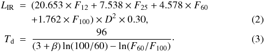 In
the equations above, D is the distance from the Sun in kpc, and the
emissivity index of dust particles β is assumed to be two. Based on the
parameters about the infrared luminosity, dust temperature in Table 3, the eight IRAS point sources are probable candidates for young
massive stars.
In
the equations above, D is the distance from the Sun in kpc, and the
emissivity index of dust particles β is assumed to be two. Based on the
parameters about the infrared luminosity, dust temperature in Table 3, the eight IRAS point sources are probable candidates for young
massive stars.
Ionizing star candidates within bubble.
In studying of the occurrence of maser emission from star-forming regions in the very early stages of evolution, Palumbo et al. (1994) found the 22 GHz H2O maser emission has a flux of less than 3.1 Jy, and van der Walt et al. (1995) did not find any 6.7 GHz methanol maser toward the IR2 (IRAS 19499+2613). Also, in a study surveying the occurrence of the 22 GHz H2O maser emission from bright IR sources in star-forming regions, Palla et al. (1991) found the peak flux of H2O maser is less than 2.7 Jy toward the IR4 (IRAS 19501+2607) near clump H.
3.7. Ionizing stars and YSOs
The GLIMPSE color−color (CC) diagram [5.8]−[8.0] versus [3.6]−[4.5] in Fig. 7a shows the distribution of class I, II, and III stars, which are located within a circle of about 10′ in radius centered on N131. Here we only considered these sources with detection in four Spitzer-IRAC bands (Hora et al. 2008). Class I sources are protostars with circumstellar envelopes; class II sources are disk dominated objects; and class III sources refer to young stars above the main sequence (and contracting towards it), but without accretion characteristics such as Hα emission (Allen et al. 2004; Petriella et al. 2010).
The reliable ionizing stars are mainly from the class III candidates and centrally distributed in a small region within the bubble, so we only considered the sources within a circle of 2.60′ (0.5 × rin) in radius centered on N131. Furthermore to get rid of the background and foreground stars, we used the 2MASS CC diagram (H − Ks) versus (J − H) in Fig. 7b. Considering the extinction in the Galactic plane as a function of distance to the Sun, Amôres & Lépine (2005) present an average Galaxy ISM extinction AV = 0.96 mag kpc-1 for one model. The adopted distance of the N131 is 8.6 kpc from the Sun, so we just considered the sources between the extinction range 10.6 ~ 6.6 mag. Finally, we obtained 15 reliable ionizing star candidates within the bubble N131. In Table 4, we report the 15 ionizing candidates within the bubble: Col. (1) specifies the GLIMPSE designation; Cols. (2)−(8) list the magnitude of four Spitzer-IRAC bands and three 2MASS JHKs bands, respectively; Col. (9) lists the ISM extinction AV; the absolute JHKs magnitude and spectral type were derived in Cols. (10)−(13).
YSOs are mainly distributed around the ringlike shell of the bubble, so we selected YSO candidates from class I and class II sources in Fig. 7a. We then excluded the potential sources belonging to the reddening main sequence and giant stars using the 2MASS CC diagram in Fig. 7b. These (class I and II) sources in Fig. 7b only include those with simultaneous detection in the four Spitzer-IRAC bands and three 2MASS JHKs bands. Finally, we found 29 class I stars and 34 class II stars as YSO candidates, which are indicated around the bubble N131 in Fig. 3. We can see that the clustered YSOs are distributed on the clouds AD and BC in the line of sight, and several YSOs are located near the molecular clumps G and H on the ringlike shell. This distribution provides some evidence for star formation triggered by the bubble. Within the bubble, there are two YSO candidates, which are possibly the background or foreground stars. We also found that there is a good correlation between the YSOs and MIPSGAL 24 μm distribution.
4. Summary
Based on our CO emission observations of 13.7-m PMO telescope, together with other archival data including GLIMPSE, MIPSGAL, 2MASS, IRAS, and NVSS, we have studied the ISM around the IR dust bubble N131. The main results can be summarized as follows.
-
1.
We found that the ringlike shell of the associated CO clouds is well correlated with the Spitzer 8.0 and 24 μm emission, and there are two giant elongated molecular clouds (AD and BC) of CO emission appearing on opposite sides of the ringlike shell of N131. The two elongated clouds may be triggered by the stellar wind from the clustered ionizing stars within the N131, but this possibility needs to be explored further.
-
2.
Contrasting the morphologic distributions between the CO and 8.0 μm emissions, we found that the CO radii agree rather well with those from the 8 μm image. DN131 = 8.6 kpc was adopted as the distance of the bubble N131 from the Sun.
-
3.
We found there is a cavity within the bubble at 1.4 GHz and 24 μm, indicating that hot dust and ionized gas have likely been evacuated by stellar wind.
-
4.
Seven IRAS point sources (IR2, IR3, ..., and IR8) are distributed along the ringlike shell of the bubble N131. IR2 (IRAS 19499+2613) is located at the peak of HII region G63.049-0.348. IR2, IR4, IR6, and IR8 are well correlated with the molecular clumps A, H, E, and G, respectively.
-
5.
We found 15 ionizing stars and 63 YSO candidates. The clustered YSOs are distributed along the elongated clouds AD and BC, and several YSOs are located around the clumps G and I. These locations may be the birth places of star formation triggered by the bubble N131.
2MASS is a joint project of the University of Massachusetts and the Infrared Processing and Analysis Center/California Institute of Technology, funded by the National Aeronautics and Space Administration and the National Science Foundation.
Acknowledgments
We wish to thank the anonymous referee and editor Malcolm Walmsley for comments and suggestions that improved the clarity of the paper. We are grateful to the staff at the Qinghai Station of PMO for their assistance during the observations. Thanks go to the Key Laboratory for Radio Astronomy, CAS, for support the operating telescope. This work was supported by the Young Researcher Grant of the National Astronomical Observatories, Chinese Academy of Sciences.
References
- Allen, L. E., Calvet, N., D’Alessio, P., et al. 2004, ApJS, 154, 363 [NASA ADS] [CrossRef] [Google Scholar]
- Amôres, E. B., & Lépine, J. R. D. 2005, AJ, 130, 659 [NASA ADS] [CrossRef] [Google Scholar]
- Beaumont, C. N., & Williams, J. P. 2010, ApJ, 709, 791 [NASA ADS] [CrossRef] [Google Scholar]
- Benjamin, R. A., Churchwell, E., Babler, B. L., et al. 2003, PASP, 115, 953 [NASA ADS] [CrossRef] [Google Scholar]
- Bessell, M. S., & Brett, J. M. 1988, PASP, 100, 1134 [NASA ADS] [CrossRef] [Google Scholar]
- Carey, S. J., Noriega-Crespo, A., Mizuno, D. R., et al. 2009, PASP, 121, 76 [NASA ADS] [CrossRef] [Google Scholar]
- Casoli, F., Combes, F., Dupraz, C., Gerin, M., & Boulanger, F. 1986, A&A, 169, 281 [NASA ADS] [Google Scholar]
- Churchwell, E., Povich, M. S., Allen, D., et al. 2006, ApJ, 649, 759 [NASA ADS] [CrossRef] [Google Scholar]
- Churchwell, E., Watson, D. F., Povich, M. S., et al. 2007, ApJ, 670, 428 [NASA ADS] [CrossRef] [Google Scholar]
- Churchwell, E., Babler, B. L., Meade, M. R., et al. 2009, PASP, 121, 213 [NASA ADS] [CrossRef] [Google Scholar]
- Condon, J. J., Cotton, W. D., Greisen, E. W., et al. 1998, AJ, 115, 1693 [NASA ADS] [CrossRef] [Google Scholar]
- Dame, T. M., Ungerechts, H., Cohen, R. S., et al. 1987, ApJ, 322, 706 [NASA ADS] [CrossRef] [Google Scholar]
- Dame, T. M., Hartmann, D., & Thaddeus, P. 2001, ApJ, 547, 792 [NASA ADS] [CrossRef] [Google Scholar]
- Deharveng, L., Schuller, F., Anderson, L. D., et al. 2010, A&A, 523, A6 [NASA ADS] [CrossRef] [EDP Sciences] [Google Scholar]
- Everett, J. E., & Churchwell, E. 2010, ApJ, 713, 592 [NASA ADS] [CrossRef] [Google Scholar]
- Fazio, G. G., Hora, J. L., Allen, L. E., et al. 2004, ApJS, 154, 10 [NASA ADS] [CrossRef] [Google Scholar]
- Furst, E., Reich, W., Reich, P., & Reif, K. 1990, A&AS, 85, 805 [NASA ADS] [Google Scholar]
- Garden, R. P., Hayashi, M., Hasegawa, T., Gatley, I., & Kaifu, N. 1991, ApJ, 374, 540 [NASA ADS] [CrossRef] [Google Scholar]
- Gregory, P. C., Scott, W. K., Douglas, K., & Condon, J. J. 1996, ApJS, 103, 427 [NASA ADS] [CrossRef] [Google Scholar]
- Henning, T., Pfau, W., & Altenhoff, W. J. 1990, A&A, 227, 542 [NASA ADS] [Google Scholar]
- Hora, J. L., Carey, S., Surace, J., et al. 2008, PASP, 120, 1233 [NASA ADS] [CrossRef] [Google Scholar]
- Ji, W.-G., Zhou, J.-J., Esimbek, J., et al. 2012, A&A, 544, A39 [NASA ADS] [CrossRef] [EDP Sciences] [Google Scholar]
- Martins, F., & Plez, B. 2006, A&A, 457, 637 [NASA ADS] [CrossRef] [EDP Sciences] [Google Scholar]
- Mezger, P. G., & Henderson, A. P. 1967, ApJ, 147, 471 [NASA ADS] [CrossRef] [Google Scholar]
- Mezger, P. G., Smith, L. F., & Churchwell, E. 1974, A&A, 32, 269 [NASA ADS] [Google Scholar]
- Neugebauer, G., Habing, H. J., van Duinen, R., et al. 1984, ApJ, 278, 1 [NASA ADS] [CrossRef] [Google Scholar]
- Palla, F., Brand, J., Comoretto, G., Felli, M., & Cesaroni, R. 1991, A&A, 246, 249 [NASA ADS] [Google Scholar]
- Palumbo, G. G. C., Scappini, F., Pareschi, G., et al. 1994, MNRAS, 266, 123 [NASA ADS] [Google Scholar]
- Panagia, N. 1973, AJ, 78, 929 [NASA ADS] [CrossRef] [Google Scholar]
- Petriella, A., Paron, S., & Giacani, E. 2010, A&A, 513, A44 [NASA ADS] [CrossRef] [EDP Sciences] [Google Scholar]
- Rieke, G. H., & Lebofsky, M. J. 1985, ApJ, 288, 618 [NASA ADS] [CrossRef] [Google Scholar]
- Simpson, R. J., Povich, M. S., Kendrew, S., et al. 2012, MNRAS, 424, 2442 [NASA ADS] [CrossRef] [Google Scholar]
- Skrutskie, M. F., Cutri, R. M., Stiening, R., et al. 2006, AJ, 131, 1163 [NASA ADS] [CrossRef] [Google Scholar]
- van der Walt, D. J., Gaylard, M. J., & MacLeod, G. C. 1995, A&AS, 110, 81 [NASA ADS] [Google Scholar]
- Watson, C., Araya, E., Sewilo, M., et al. 2003, ApJ, 587, 714 [NASA ADS] [CrossRef] [Google Scholar]
- Watson, C., Povich, M. S., Churchwell, E. B., et al. 2008, ApJ, 681, 1341 [NASA ADS] [CrossRef] [Google Scholar]
- Watson, C., Corn, T., Churchwell, E. B., et al. 2009, ApJ, 694, 546 [NASA ADS] [CrossRef] [Google Scholar]
- Watson, C., Hanspal, U., & Mengistu, A. 2010, ApJ, 716, 1478 [NASA ADS] [CrossRef] [Google Scholar]
- Werner, M. W., Roellig, T. L., Low, F. J., et al. 2004, ApJS, 154, 1 [Google Scholar]
- Winnewisser, G., Churchwell, E., & Walmsley, C. M. 1979, A&A, 72, 215 [NASA ADS] [Google Scholar]
- Zavagno, A., Anderson, L. D., Russeil, D., et al. 2010, A&A, 518, L101 [NASA ADS] [CrossRef] [EDP Sciences] [Google Scholar]
- Zhang, C. P., & Wang, J. J. 2012a, A&A, 544, A11 [NASA ADS] [CrossRef] [EDP Sciences] [Google Scholar]
- Zhang, C.-P., & Wang, J.-J. 2012b, RAA, 13, 47 [Google Scholar]
All Tables
All Figures
|
Fig. 1 12CO (red line), 13CO (black line), and C18O (green line) spectra at the peaks of the molecular clumps from A to I. The brightness temperature of each 13CO spectrum is multiplied by 2. |
| In the text | |
|
Fig. 2 Integrated intensity contours of the 12CO emission clouds superimposed on the GLIMPSE 8.0 μm colorscale. The contour levels range from 5.35 to 32.11 by 2.68 K km s-1. The integration range is from −14.5 to −6.5 km s-1. The letters from A to I indicate the positions of nine molecular clumps, and the area of each clump is indicated with dashed ellipse and polygon. The black symbols “■” indicate the positions of IRAS point sources. The white ellipse indicates the position of bubble N131, and the straight lines indicate the position of position-velocity diagram in Fig. 5. The beam size of 12CO emission is given in the filled red circle. The unit of the color bar is in MJy sr-1. |
| In the text | |
|
Fig. 3 Integrated intensity contours of the 13CO emission clouds superimposed on the MIPSGAL 24 μm colorscale. The contour levels range from 2.17 to 8.68 by 1.09 K km s-1. The integration range is from −14.5 to −6.5 km s-1. The letters from A to I indicate the positions of nine molecular clumps, and the symbols “”, “ × ”, and “■” indicate the positions of class I, class II, and IRAS point sources, respectively. The white ellipse indicates the position of bubble N131. The beam size of 12CO emission is given in the filled red circle. The unit of the color bar is in MJy sr-1. |
| In the text | |
|
Fig. 4 Integrated intensity contours of the 12CO emission clouds every 1.0 km s-1 superimposed on the GLIMPSE 8.0 μm grayscale. The lowest contour level for each velocity panel from −14.5 to −6.5 km s-1 is 1.59, 1.37, 1.80, 2.24, 1.96, 2.19, 2.80, 1.22, and 0.95 K km s-1, respectively; the level increment of each panel is equal to the corresponding value of the lowest contour level. The blue, green, and red contours indicate the blueshifted, systematic, and redshifted velocities, respectively. The white ellipse indicates the position of bubble N131. |
| In the text | |
|
Fig. 5 Position-velocity diagram of the 12CO emission clouds along the white
straight lines in Fig. 2. The position
corresponding to offset 0 is at RA(J2000) =
19h52m17 |
| In the text | |
|
Fig. 6 Integrated intensity contours of the 12CO emission of the blueshifted and redshifted clouds superimposed on the 1.4 GHz NVSS continuum emission contours. The contour levels range from 3.20 to 19.20 by 1.60 K for the blueshifted cloud, and from 3.86 to 23.17 by 1.93 K for the redshifted cloud. The integration range is from −14.5 to −11.5 km s-1 for blueshifted cloud, and from −9.5 to −6.5 km s-1 for redshifted cloud. The contour levels of the 1.4 GHz NVSS continuum emission are 0.95, 1.26, 1.58, 3.16, 6.32, 12.64, 25.29, and 50.58 mJy beam-1. G63.049-0.348 is an HII region. The letters from A to I indicate the positions of nine molecular clumps, and the symbols “■” indicate the positions of IRAS point sources. The green ellipse indicates the position of bubble N131. The beam size of 12CO emission is given in the filled black circle. |
| In the text | |
|
Fig. 7 a) GLIMPSE CC diagram [5.8]−[8.0] versus [3.6]−[4.5] for sources within a circle of about 10′ in radius centered on N131. The classification of class I, II, and III indicates different stellar evolutionary stages as defined by Allen et al. (2004). b) 2MASS CC diagram (H − Ks) versus (J − H). The sources for classes I and II are these, detected simultaneously by J, H, Ks, 3.6, 4.5, 5.8, and 8.0 μ bands; the sources for class III are located within a circle of 2.60′ (0.5 × rin) in a radius centered on N131. The gray squares represent the location of the main sequence and the giant stars (Bessell & Brett 1988). The parallel dotted lines are reddening vectors. The adopted interstellar reddening law is AJ / AV = 0.282, AH / AV = 0.175, and AKs / AV = 0.112 (Rieke & Lebofsky 1985), and the intrinsic colors (H − Ks)0 and (J − H)0 are obtained from Martins & Plez (2006). |
| In the text | |
Current usage metrics show cumulative count of Article Views (full-text article views including HTML views, PDF and ePub downloads, according to the available data) and Abstracts Views on Vision4Press platform.
Data correspond to usage on the plateform after 2015. The current usage metrics is available 48-96 hours after online publication and is updated daily on week days.
Initial download of the metrics may take a while.